Energy Efficient Pico Cell Range Expansion and Density Joint Optimization for Heterogeneous Networks with eICIC

Abstract
1. Introduction
1.1. Motivation
1.2. Related Works
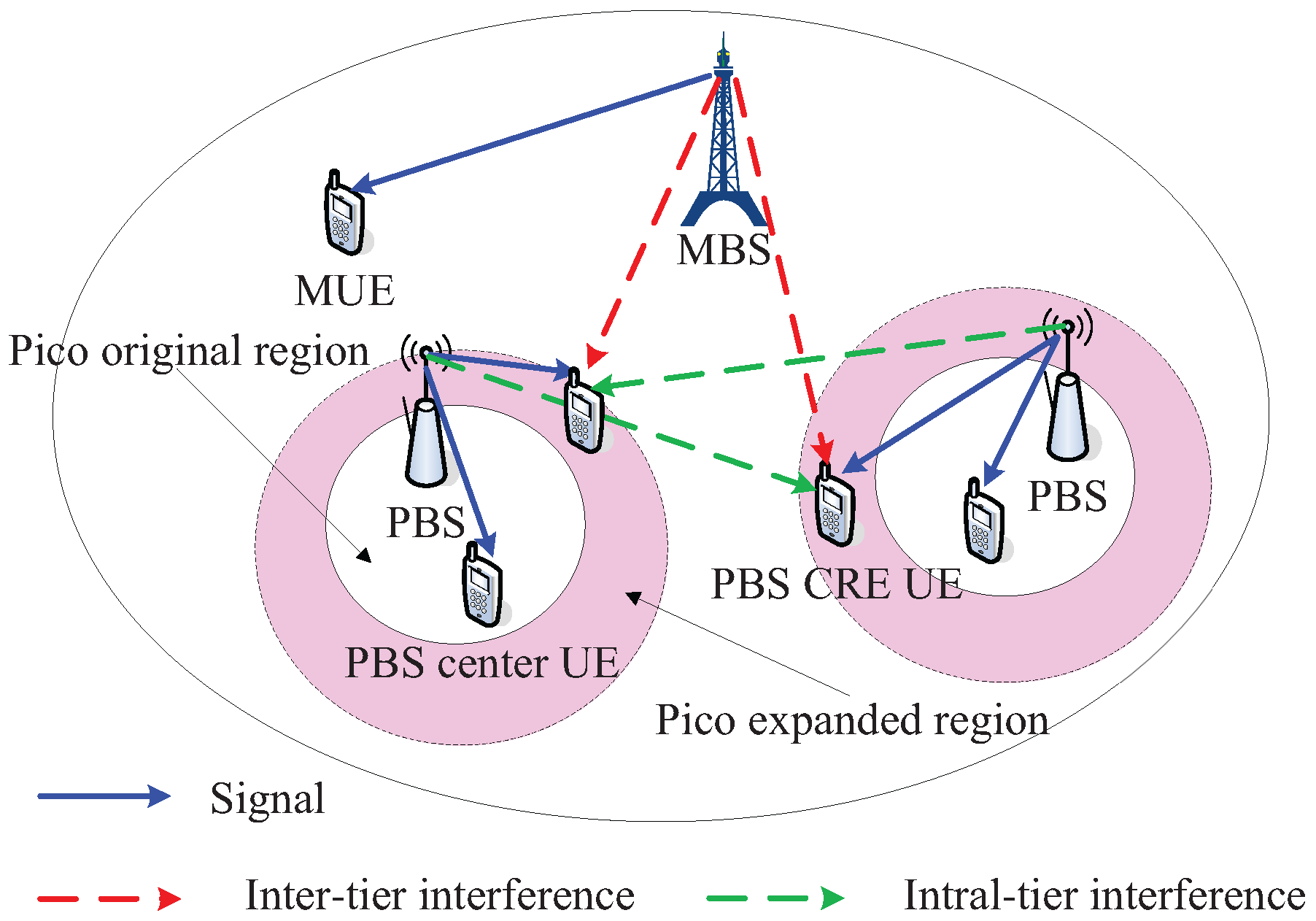
2. Network Model
3. Analytical Model
3.1. User Type Probability
3.2. Distribution of Serving BS Distance
3.3. The Ratio of Almost Blank Subframe
3.4. Average Ergodic Rate
3.5. BS Power Consumption
3.6. Network Energy Efficiency
4. Joint Parameters Optimization
4.1. Optimization of Pico CRE Bias
| Algorithm 1: CRE Bias Optimization (CBO) Algorithm. | |
| 1. Initialization: (1) Initialize the network scenario and the values , and , where . (2) Set the initial value of . (3) Denote as the variable step length of . Denote as the optimal value of the network EE. Denote as the optimized CRE bias. Let , and . 2. Calculate the optimal pico CRE bias while do according to Equation (14) if then , end if end while | |
4.2. Optimization of PBS Density
| Algorithm 2: PBS Density Optimization (PDO) Algorithm. | |
| 1. Initialization: (1) Initialize the network scenario and the values , and , where . (2) Set the initial value of . (3) Denote as the variable step length of . Denote as the optimal value of the network EE. Denote as the optimized ratio between PBS density MBS density. Let , and . 2. Calculate the optimal ratio of PBS density to MBS density while do according to Equation (14) if then , end if end while 3. Obtain the optimal PBS density | |
4.3. Joint Optimization of Pico CRE Bias and PBS Density
| Algorithm 3: Joint Pico CRE Bias and PBS Density Optimization (JBPDO) Algorithm. | |
| 1. Initialization: (1) Initialize the network scenario and the values , , and , where and . (2) Let represent the initial optimal value of the network EE. Initialize algorithm iteration number . Given a tolerance . (3) Denote as the optimized PBS CRE bias. Denote as the optimized ratio of PBS density to MBS density. Denote as the optimized PBS density. 2. Calculate the suboptimal CRE bias according to CBO Algorithm 3. Calculate the suboptimal ratio of PBS density to MBS density according to PDO Algorithm 4. Termination of the loop if then , , go to step 2 else , , end if | |
5. Numerical Results and Analysis
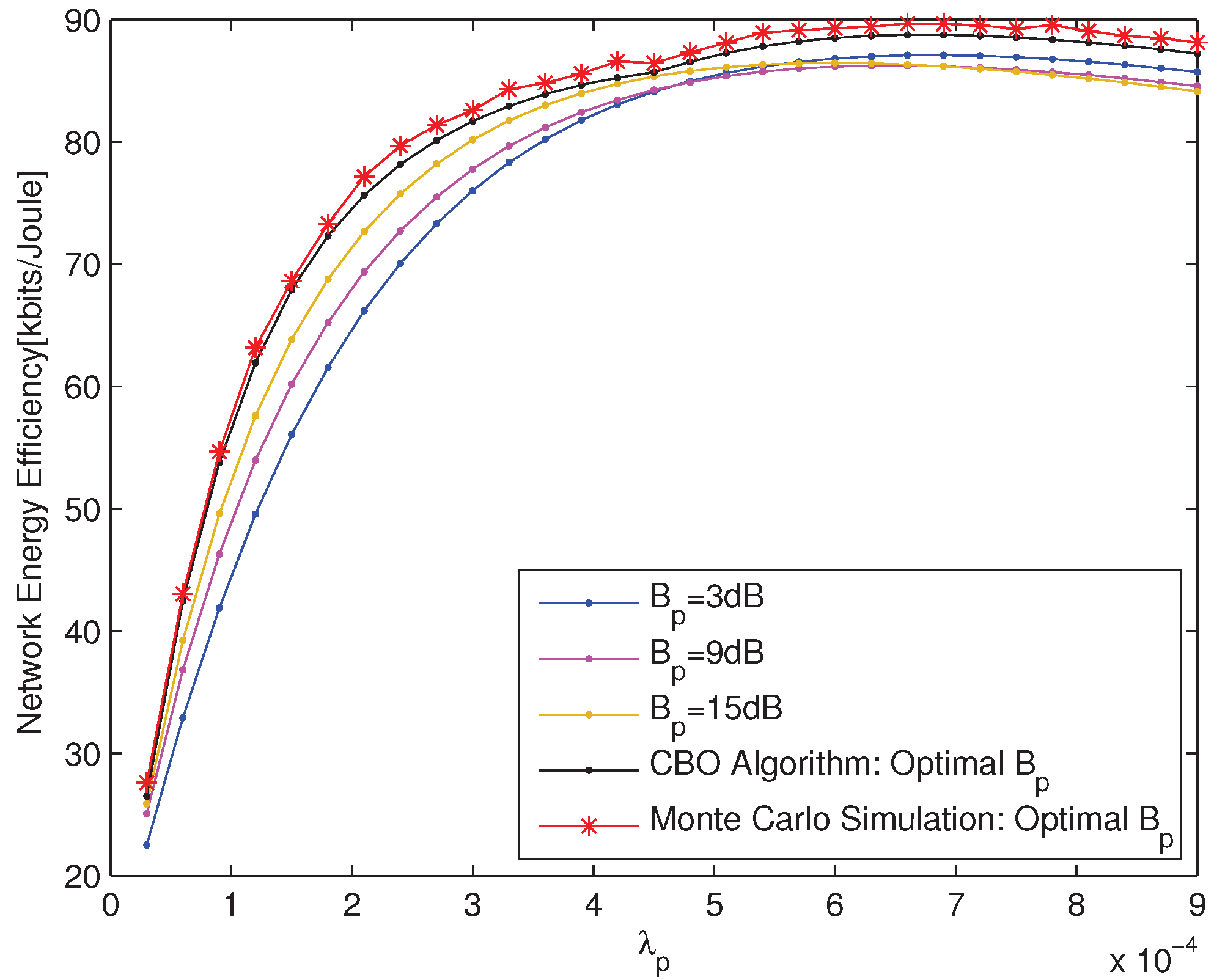
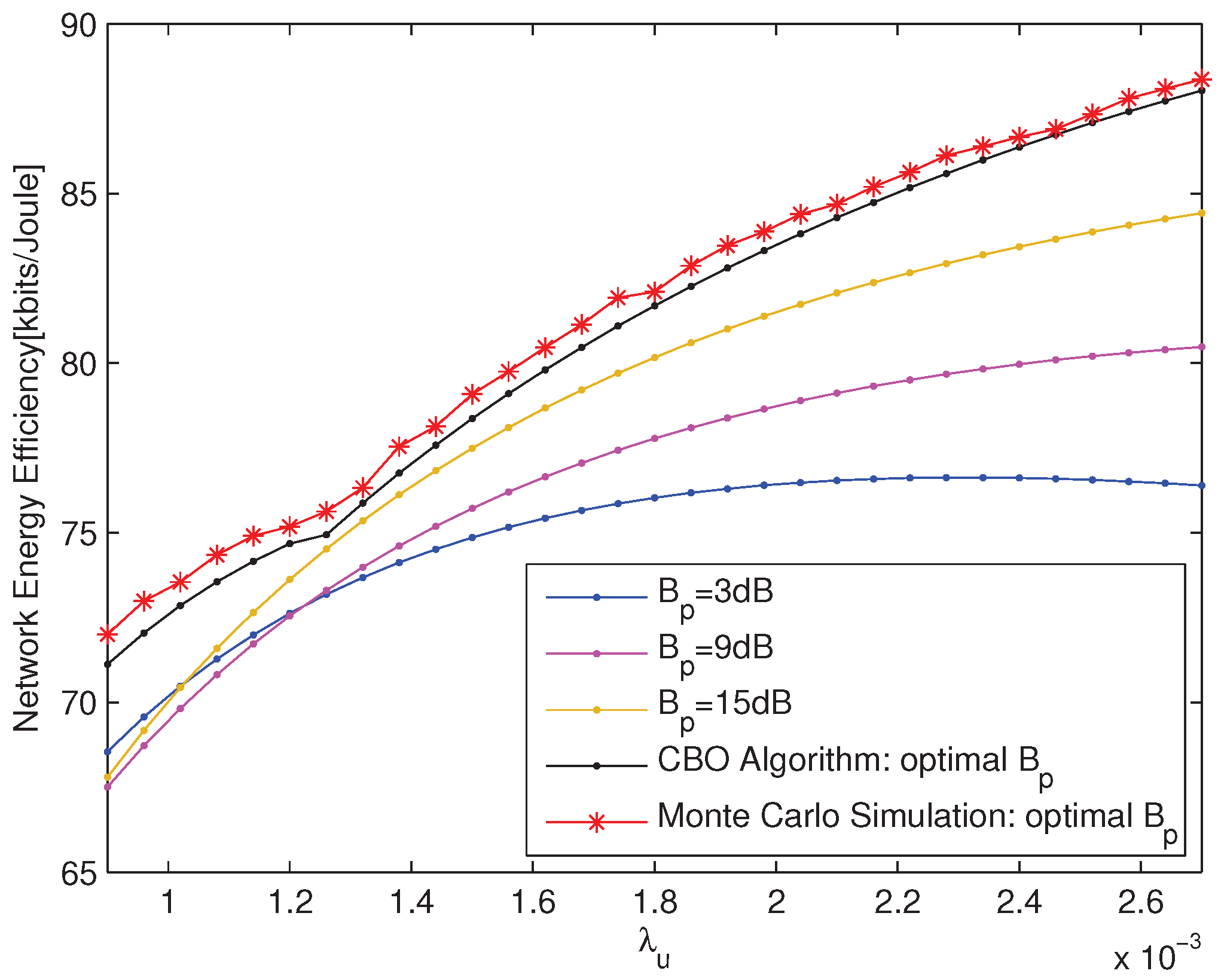
5.1. Performance Analysis for Pico CRE Bias Optimization
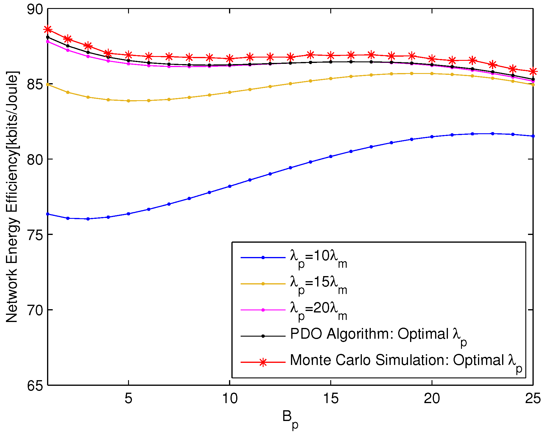
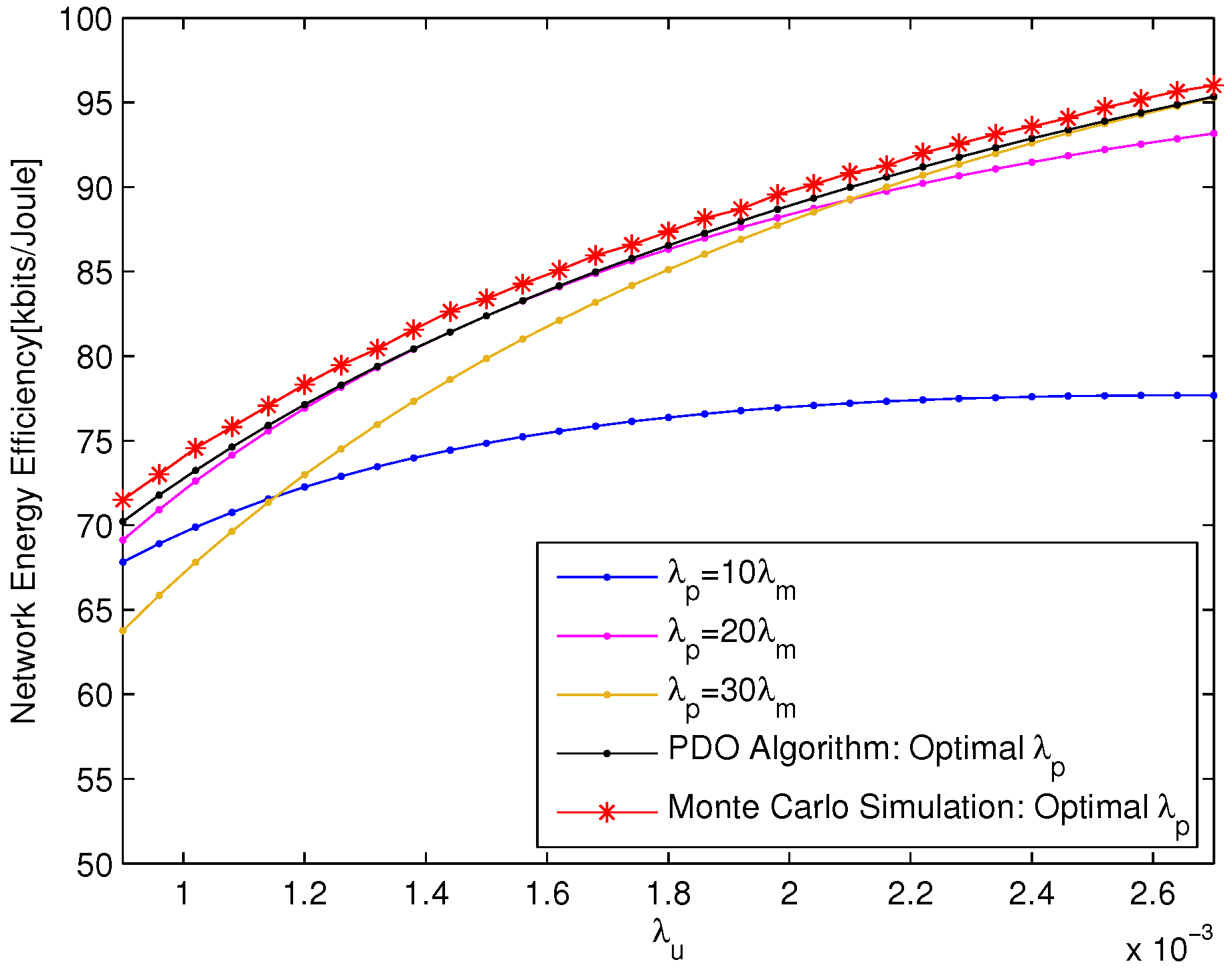
5.2. Performance Analysis for PBS Density Optimization
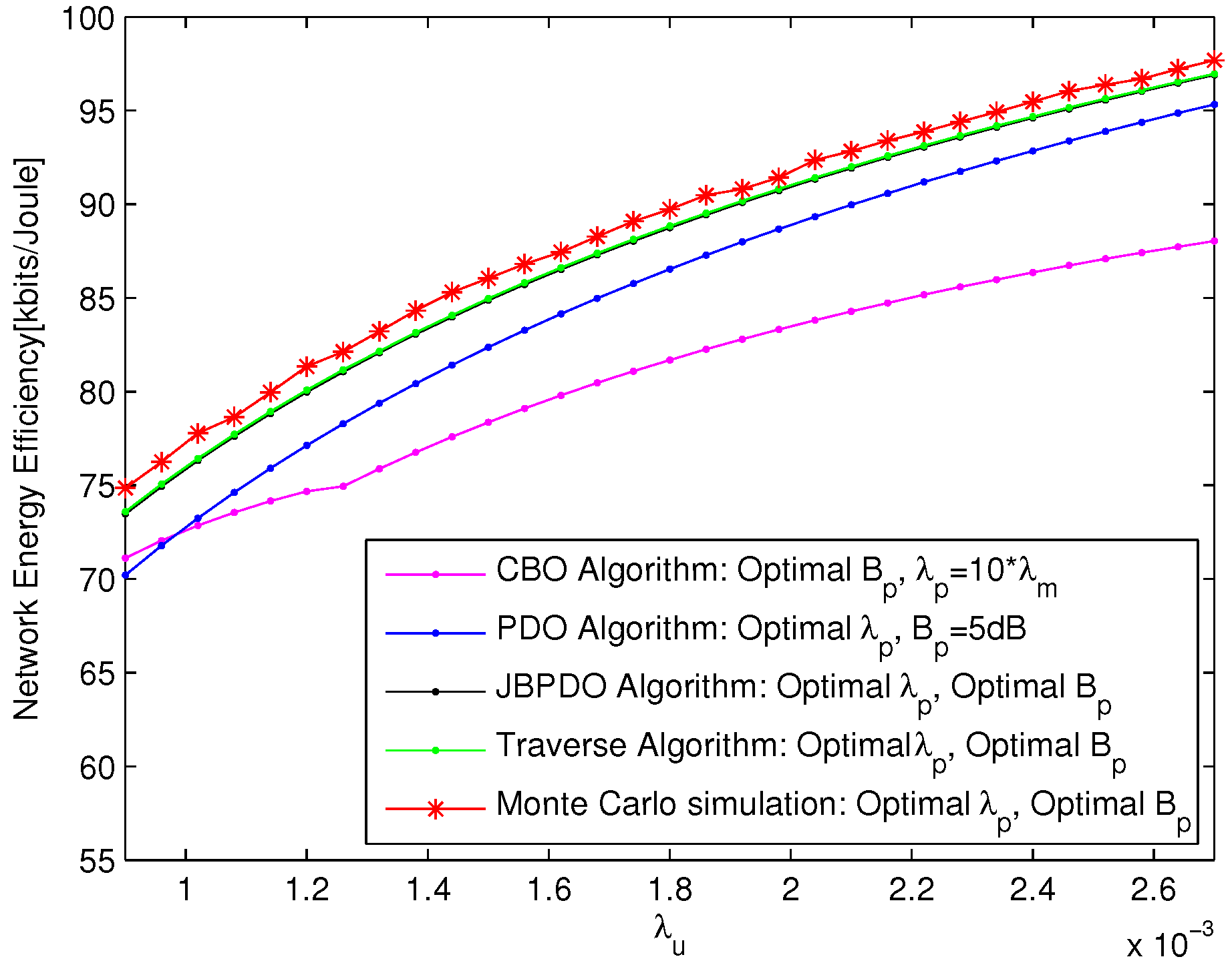
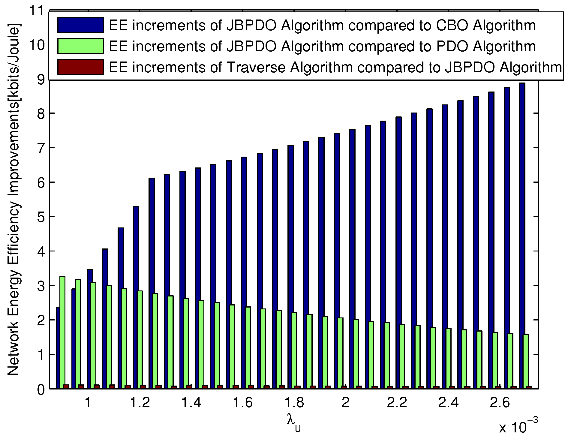
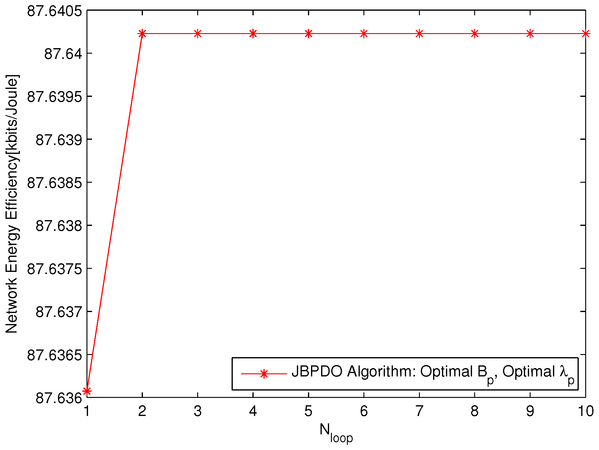
5.3. Performance Analysis for Joint Optimization of CRE Bias and PBS Density
6. Conclusions
Acknowledgments
Author Contributions
Conflicts of Interest
Appendix A
Appendix B
Appendix C
References
- Zhang, S.; Wu, Q.; Xu, S.; Li, G.Y. Fundamental Green Tradeoffs: Progresses, Challenges, and Impacts on 5G Networks. IEEE Commun. Surv. Tutor. 2017, 19, 33–56. [Google Scholar] [CrossRef]
- Wu, G.; Yang, C.; Li, S.; Li, G.Y. Recent advances in energy-efficient networks and their application in 5G systems. IEEE Wirel. Commun. 2015, 22, 145–151. [Google Scholar] [CrossRef]
- Zhang, T.; Zhao, J.; An, L.; Liu, D. Energy efficiency of base station deployment in ultra dense hetnets: A stochastic geometry analysis. IEEE Wirel. Commun. Lett. 2016, 5, 184–187. [Google Scholar] [CrossRef]
- Sun, Y.; Xu, L.; Wu, Y.; Wang, T.; Fang, Y. Energy Efficient Small Cell Density Optimization Based on Stochastic Geometry in Ultra-Dense HetNets. In Proceedings of the IEEE International Conference on Communication Software and Networks (ICCSN), Guangzhou, China, 6–8 May 2017; pp. 1–6. [Google Scholar]
- Sun, Y.; Wang, Z.; Wang, T.; Wu, Y.; Fang, Y. Joint Optimization of Parameters for Enhanced Inter-Cell Interference Coordination (eICIC) in LTE-A HetNets. IEICE Trans. Commun. 2017, 100, 799–807. [Google Scholar] [CrossRef]
- Hu, R.Q.; Qian, Y.; Kota, S.; Giambene, G. HetNets-a new paradigm for increasing cellular capacity and coverage. IEEE Wirel. Commun. 2011, 18, 8–9. [Google Scholar] [CrossRef]
- Kamel, M.; Hamouda, W.; Youssef, A. Ultra-dense networks: A survey. IEEE Commun. Surv. Tutor. 2016, 18, 2522–2545. [Google Scholar] [CrossRef]
- Bhushan, N.; Li, J.; Malladi, D.; Gilmore, R.; Brenner, D.; Damnjanovic, A.; Sukhavasi, R.T.; Patel, C.; Geirhofer, S. Network densification: the dominant theme for wireless evolution into 5G. IEEE Commun. Mag. 2014, 52, 82–89. [Google Scholar] [CrossRef]
- Yamamoto, K.; Ohtsuki, T. Parameter optimization using local search for CRE and eICIC in heterogeneous network. In Proceedings of the IEEE International Symposium on Personal, Indoor, and Mobile Radio Communication (PIMRC), Washington, DC, USA, 2–5 September 2014; pp. 1536–1540. [Google Scholar]
- Singh, S.; Dhillon, H.S.; Andrews, J.G. Offloading in Heterogeneous Networks: Modeling, Analysis, and Design Insights. IEEE Trans. Wirel. Commun. 2013, 12, 2484–2497. [Google Scholar] [CrossRef]
- Lopez-Perez, D.; Guvenc, I.; Roche, G.D.L.; Kountouris, M.; Quek, T.Q.S.; Zhang, J. Enhanced intercell interference coordination challenges in heterogeneous networks. IEEE Wirel. Commun. 2011, 18, 22–30. [Google Scholar] [CrossRef]
- Deb, S.; Monogioudis, P.; Miernik, J.; Seymour, J.P. Algorithms for Enhanced Inter-Cell Interference Coordination (eICIC) in LTE HetNets. IEEE/ACM Trans. Netw. 2014, 22, 137–150. [Google Scholar] [CrossRef]
- Feng, D.; Jiang, C.; Lim, G.; Cimini, L.J.; Feng, G.; Li, G.Y. A survey of energy-efficient wireless communications. IEEE Commun. Surv. Tutor. 2013, 15, 167–178. [Google Scholar] [CrossRef]
- Chen, X.; Xia, H.; Zeng, Z.; Wu, S.; Zuo, W.; Lu, Y. Energy-efficient heterogeneous networks for green communications by inter-layer interference coordination. In Proceedings of the IEEE International Symposium on Wireless Personal Multimedia Communications (WPMC), Sydney, NSW, Australia, 7–10 September 2014; pp. 70–74. [Google Scholar]
- Kuang, Q.; Utschick, W. Energy Management in Heterogeneous Networks With Cell Activation, User Association, and Interference Coordination. IEEE Trans. Wirel. Commun. 2016, 15, 3868–3879. [Google Scholar] [CrossRef]
- Hu, H.; Weng, J.; Zhang, J. Coverage Performance Analysis of FeICIC Low-Power Subframes. IEEE Trans. Wirel. Commun. 2016, 15, 5603–5614. [Google Scholar] [CrossRef]
- Singh, S.; Andrews, J.G. Joint Resource Partitioning and Offloading in Heterogeneous Cellular Networks. IEEE Trans. Wirel. Commun. 2014, 13, 888–901. [Google Scholar] [CrossRef]
- Bu, S.; Yu, F.R.; Yanikomeroglu, H. Interference-aware energy-efficient resource allocation for heterogeneous networks with incomplete channel state information. IEEE Trans. Veh. Technol. 2015, 64, 1036–1050. [Google Scholar] [CrossRef]
- Wang, Y.; Wang, X.; Shi, J. A Stackelberg Game Approach for Energy efficient Resource Allocation and Interference Coordination in Heterogeneous Networks. In Proceedings of the IEEE International Conference on Computer and Information Technology, Xi’an, China, 11–13 September 2014; pp. 694–699. [Google Scholar]
- Wang, Z.; Hu, B.; Wang, X.; Chen, S. Interference pricing in 5G ultra-dense small cell networks: A Stackelberg game approach. IET Commun. 2016, 10, 1865–1872. [Google Scholar] [CrossRef]
- Al-Zahrani, A.Y.; Yu, F.R. An Energy-Efficient Resource Allocation and Interference Management Scheme in Green Heterogeneous Networks Using Game Theory. IEEE Trans. Veh. Technol. 2016, 65, 5384–5396. [Google Scholar] [CrossRef]
- Yang, C.; Li, J.; Ni, Q.; Anpalagan, A.; Guizani, M. Interference-Aware Energy Efficiency Maximization in 5G Ultra-Dense Networks. IEEE Trans. Commun. 2017, 65, 728–739. [Google Scholar] [CrossRef]
- Jiang, J.; Peng, M.; Zhang, K.; Li, L. An effective interference management framework to achieve energy-efficient communications for heterogeneous network through cognitive sensing. In Proceedings of the IEEE International ICST Conference on Communications and Networking in China, Kunming, China, 8–10 August 2012; pp. 536–541. [Google Scholar]
- Hou, S.; Zhang, X.; Zheng, H.; Zhao, L.; Fang, W. Energy-efficient resource allocation in heterogeneous network with cross-tier interference constraint. In Proceedings of the IEEE International Symposium on Personal, Indoor and Mobile Radio Communications (PIMRC Workshops), London, UK, 8–9 Septmber 2013; pp. 168–172. [Google Scholar]
- Wang, M.; Xia, H.; Feng, C. Joint eICIC and dynamic point blanking for energy-efficiency in heterogeneous network. In Proceedings of the IEEE International Conference on Wireless Communications Signal Processing (WCSP), Nanjing, China, 15–17 October 2013; pp. 168–172. [Google Scholar]
- Ge, X.; Tu, S.; Mao, G.; Wang, C.X.; Han, T. 5G Ultra-Dense Cellular Networks. IEEE Wirel. Commun. 2016, 23, 72–79. [Google Scholar] [CrossRef]
- Lin, X.; Wang, S. Joint user association and base station switching on/off for green heterogeneous cellular networks. In Proceedings of the IEEE International Conference on Communications (ICC), Paris, France, 21–25 May 2017; pp. 1–6. [Google Scholar]
- Li, L.; Peng, M.; Yang, C.; Wu, Y. Optimization of Base-Station Density for High Energy-Efficient Cellular Networks With Sleeping Strategies. IEEE Trans. Veh. Technol. 2016, 65, 7501–7514. [Google Scholar] [CrossRef]
- DiRenzo, M.; Zappone, A.; Tu, T.; Debbah, M. System-Level Modeling and Optimization of the Energy Efficiency in Cellular Networks—A Stochastic Geometry Framework. Available online: https://arxiv.org/abs/1801.07513 (accessed on 28 February 2018).
- Zhang, J.; Xiang, L.; Ng, D.W.K.; Jo, M.; Chen, M. Energy Efficiency Evaluation of Multi-Tier Cellular Uplink Transmission Under Maximum Power Constraint. IEEE Trans. Wirel. Commun. 2017, 16, 7092–7107. [Google Scholar] [CrossRef]
- Ngo, H.Q.; Larsson, E.G.; Marzetta, T.L. Energy and Spectral Efficiency of Very Large Multiuser MIMO Systems. IEEE Trans. Wirel. Commun. 2013, 61, 1436–1449. [Google Scholar]
- Cui, S.; Goldsmith, A.J.; Bahai, A. Energy-efficiency of MIMO and cooperative MIMO techniques in sensor networks. IEEE J. Sel. Areas Commun. 2004, 22, 1089–1098. [Google Scholar] [CrossRef]
- Chen, X.; Wang, X.; Chen, X. Energy-Efficient Optimization for Wireless Information and Power Transfer in Large-Scale MIMO Systems Employing Energy Beamforming. IEEE Wirel. Commun. Lett. 2013, 2, 667–670. [Google Scholar] [CrossRef]
- Bjornson, E.; Kountouris, M.; Debbah, M. Massive MIMO and small cells: Improving energy efficiency by optimal soft-cell coordination. In Proceedings of the IEEE International Conference on Telecommunications (ICT), Casablanca, Morocco, 6–8 May 2013; pp. 1–5. [Google Scholar]
- Lee, B.M.; Yang, H. Massive MIMO for Industrial Internet of Things in Cyber-Physical Systems. IEEE Trans. Ind. Informat. 2017. [Google Scholar] [CrossRef]
- Onireti, O.; Heliot, F.; Imran, M.A. On the Energy Efficiency-Spectral Efficiency Trade-Off of Distributed MIMO Systems. IEEE Trans. Commun. 2013, 61, 3741–3753. [Google Scholar] [CrossRef]
- Zhao, G.; Chen, S.; Zhao, L.; Hanzo, L. Joint Energy-Spectral-Efficiency Optimization of CoMP and BS Deployment in Dense Large-Scale Cellular Networks. IEEE Trans. Wirel. Commun. 2017, 16, 4832–4847. [Google Scholar] [CrossRef]
- Andrews, J.G.; Baccelli, F.; Ganti, R.K. A Tractable Approach to Coverage and Rate in Cellular Networks. IEEE Trans. Commun. 2011, 59, 3122–3134. [Google Scholar] [CrossRef]
- Jo, H.S.; Sang, Y.J.; Xia, P.; Andrews, J.G. Heterogeneous Cellular Networks with Flexible Cell Association: A Comprehensive Downlink SINR Analysis. IEEE Trans. Wirel. Commun. 2012, 11, 3484–3495. [Google Scholar] [CrossRef]
- An, L.; Zhang, T.; Feng, C. Joint optimization for base station density and user association in energy-efficient cellular networks. In Proceedings of the IEEE International Symposium on Wireless Personal Multimedia Communications (WPMC), Sydney, NSW, Australia, 7–10 September 2014; pp. 85–90. [Google Scholar]
- Tang, W.; Feng, S.; Liu, Y.; Reed, M.C. Joint Low-Power Transmit and Cell Association in Heterogeneous Networks. In Proceedings of the IEEE Global Communications Conference (GLOBECOM), San Diego, CA, USA, 6–10 December 2015; pp. 1–6. [Google Scholar]
- Singh, S.; Andrews, J.G. Rate distribution in heterogeneous cellular networks with resource partitioning and offloading. In Proceedings of the IEEE Global Communications Conference (GLOBECOM), Atlanta, GA, USA, 9–13 December 2013; pp. 3796–3801. [Google Scholar]
- He, G.; Zhang, S.; Chen, Y.; Xu, S. Energy efficiency and deployment efficiency tradeoff for heterogeneous wireless networks. In Proceedings of the IEEE Global Communications Conference (GLOBECOM), Anaheim, CA, USA, 3–7 December 2012; pp. 3189–3194. [Google Scholar]
- He, G.; Zhang, S.; Chen, Y.; Xu, S. Spectrum efficiency and energy efficiency tradeoff for heterogeneous wireless networks. In Proceedings of the IEEE Wireless Communications and Networking Conference (WCNC), Shanghai, China, 7–10 April 2013; pp. 2570–2574. [Google Scholar]


| Parameters | Value |
|---|---|
| Carrier frequency f | 2 GHz |
| Path loss exponent | 4 |
| Path Loss L | , where , |
| MBS transmit power or | 43 dBm or 20 W |
| PBS transmit power or | 30 dBm or 1 W |
| Bandwidth W | 10 MHz |
| MBS static power | 800 W |
| PBS static power | 130 W |
| MBS density |
© 2018 by the authors. Licensee MDPI, Basel, Switzerland. This article is an open access article distributed under the terms and conditions of the Creative Commons Attribution (CC BY) license (http://creativecommons.org/licenses/by/4.0/).
Share and Cite
Sun, Y.; Xia, W.; Zhang, S.; Wu, Y.; Wang, T.; Fang, Y. Energy Efficient Pico Cell Range Expansion and Density Joint Optimization for Heterogeneous Networks with eICIC. Sensors 2018, 18, 762. https://doi.org/10.3390/s18030762
Sun Y, Xia W, Zhang S, Wu Y, Wang T, Fang Y. Energy Efficient Pico Cell Range Expansion and Density Joint Optimization for Heterogeneous Networks with eICIC. Sensors. 2018; 18(3):762. https://doi.org/10.3390/s18030762
Chicago/Turabian StyleSun, Yanzan, Wenqing Xia, Shunqing Zhang, Yating Wu, Tao Wang, and Yong Fang. 2018. "Energy Efficient Pico Cell Range Expansion and Density Joint Optimization for Heterogeneous Networks with eICIC" Sensors 18, no. 3: 762. https://doi.org/10.3390/s18030762
APA StyleSun, Y., Xia, W., Zhang, S., Wu, Y., Wang, T., & Fang, Y. (2018). Energy Efficient Pico Cell Range Expansion and Density Joint Optimization for Heterogeneous Networks with eICIC. Sensors, 18(3), 762. https://doi.org/10.3390/s18030762