Tensor Approach to DOA Estimation of Coherent Signals with Electromagnetic Vector-Sensor Array


Abstract
1. Introduction
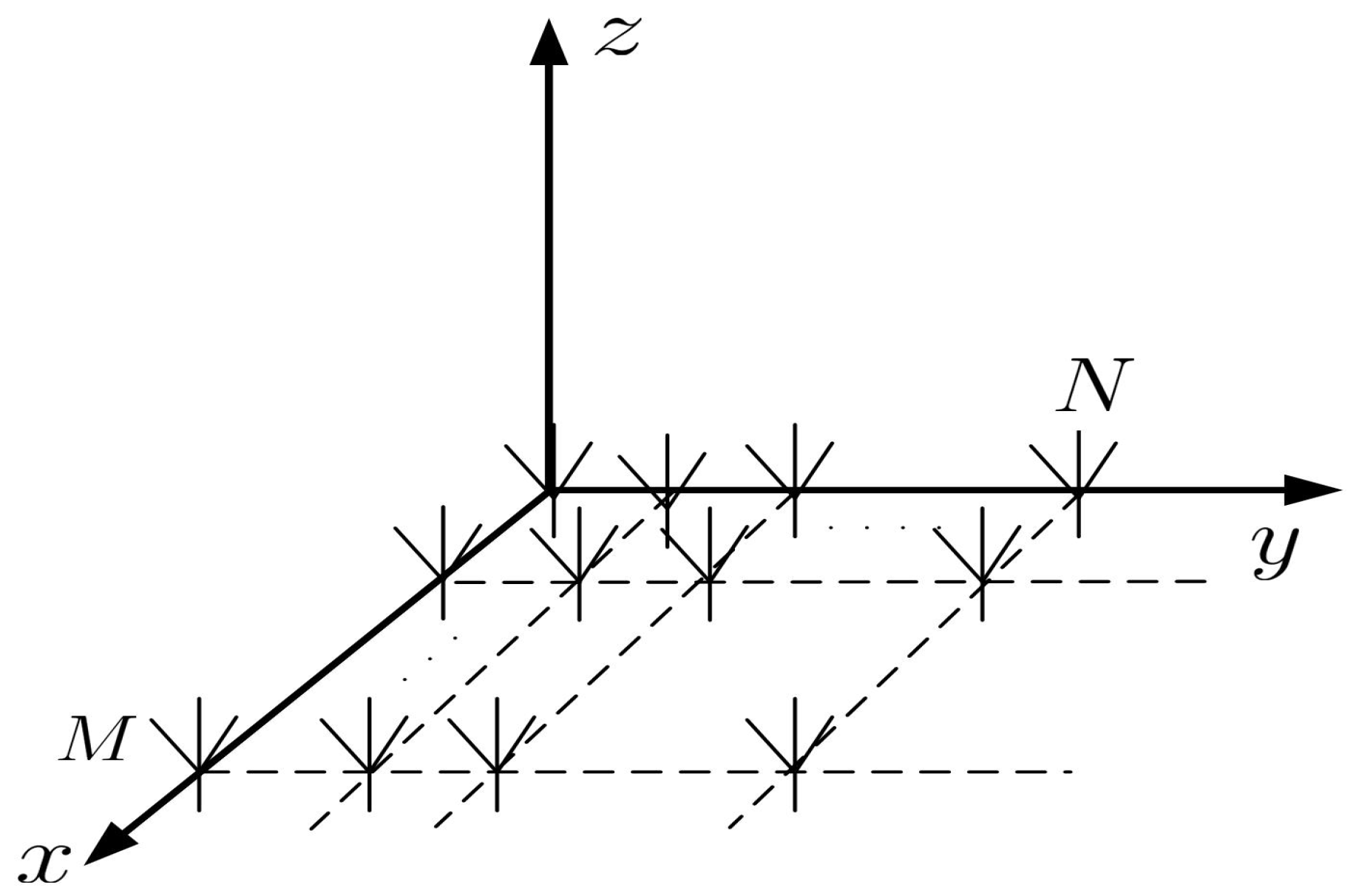
2. Signal Model
3. Tensor Approach
3.1. Tensor Notations
3.2. Tensor Modeling
3.3. DOA Estimation Methods
3.4. Polarization Parameters Estimation
4. Performance Analysis
4.1. Derivation of CRB
4.2. Array Elements’ Position Errors
4.3. Mutual Coupling Effect
4.4. Performance Analysis of the Proposed Methods
4.5. Computational Complexity Analysis
5. Simulations
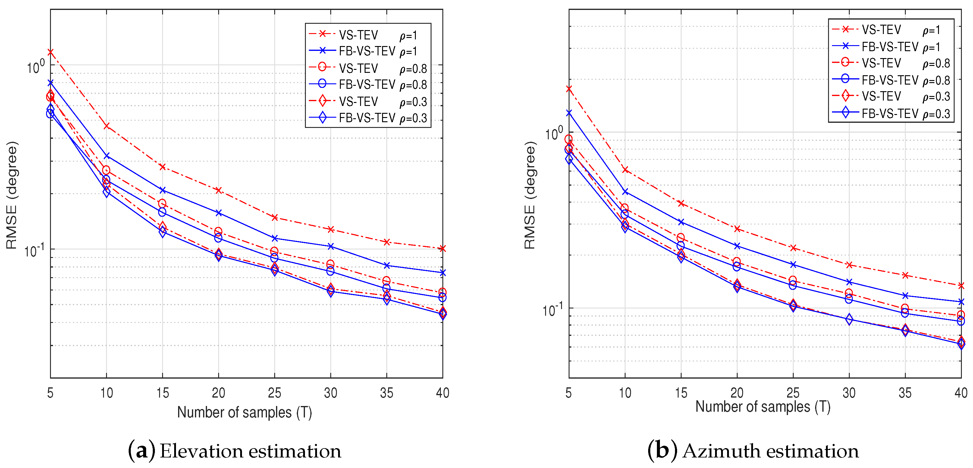
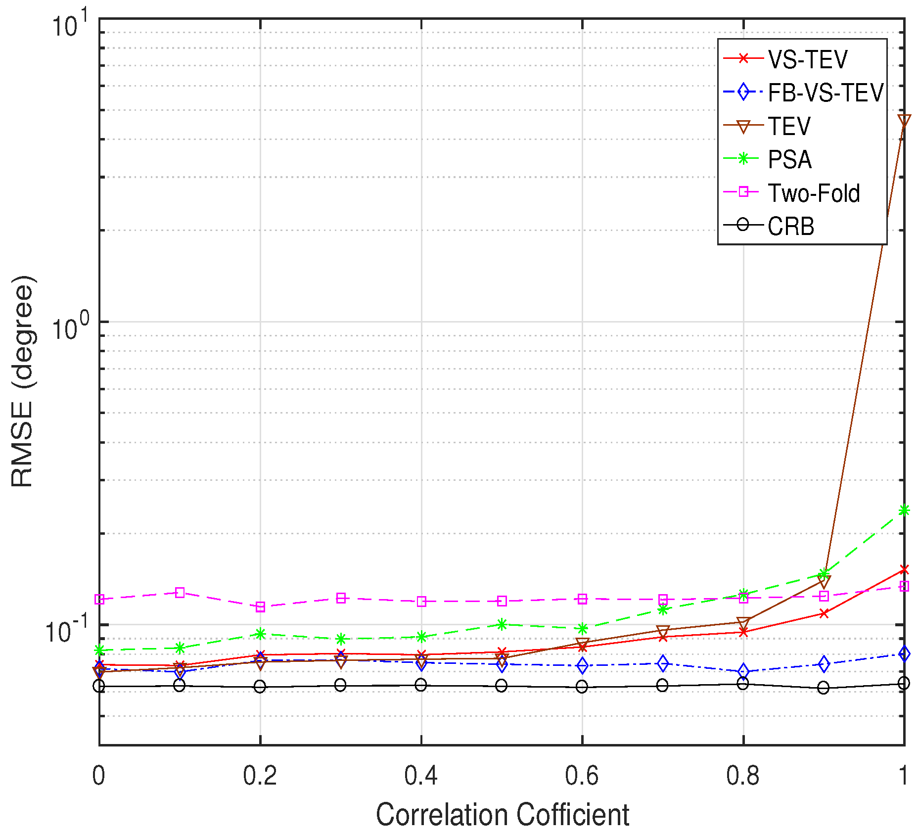
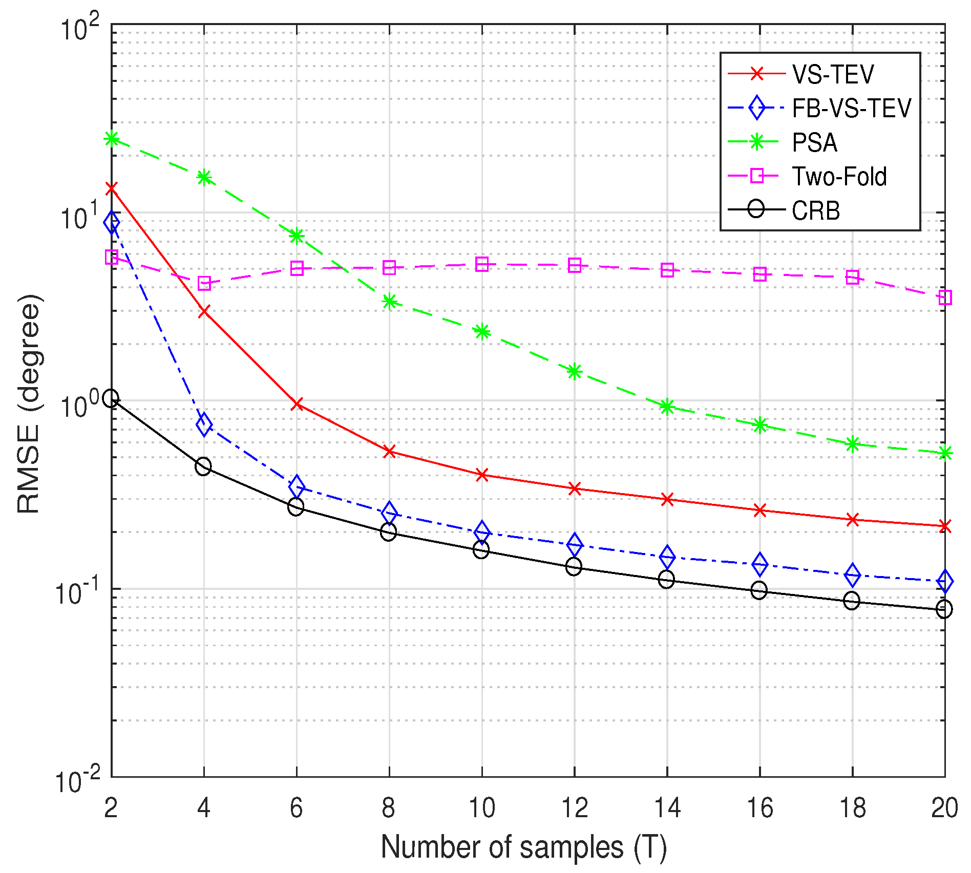
5.1. The Case of Coherent Signals
5.2. The Case of Noncoherent Signals
5.3. The Case of Unideal Electromagnetic Vector-Sensor Array
6. Conclusions
Author Contributions
Funding
Conflicts of Interest
References
- Mao, X.P.; Liu, A.J.; Hou, H.J.; Hong, H.; Guo, R. Oblique projection polarisation filtering for interference suppression in high-frequency surface wave radar. IET Radar Sonar Navig. 2012, 6, 71–80. [Google Scholar] [CrossRef]
- Yuan, X. Estimating the DOA and the polarization of a polynomial-phase signal using a single polarized vector-sensor. IEEE Trans. Signal Process. 2012, 60, 1270–1282. [Google Scholar] [CrossRef]
- Wong, K.T. Direction finding/polarization estimation-dipole and/or loop triad(s). IEEE Trans. Aerosp. Electron. Syst. 2001, 37, 679–684. [Google Scholar] [CrossRef]
- Wong, K.T.; Zoltowski, M.D. Uni-vector-sensor ESPRIT for multisource azimuth, elevation, and polarization estimation. IEEE Trans. Antennas Propag. 1997, 45, 1467–1474. [Google Scholar] [CrossRef]
- Zoltowski, M.D.; Wong, K.T. ESPRIT-based 2-D direction finding with a sparse uniform array of electromagnetic vector sensors. IEEE Trans. Signal Process. 2000, 48, 2195–2204. [Google Scholar] [CrossRef]
- Srinivasarao, C.; Palanisamy, P. 2D-DOD and 2D-DOA estimation using the electromagnetic vector sensors. Signal Process. 2018, 147, 163–172. [Google Scholar]
- Bull, J.F. Field Probe for Measuring Vector Components of an Electromagnetic Field. U.S. Patent 300 885, 5 June 1995. [Google Scholar]
- Hatke, G.F. Performance Analysis of the SuperCART Antenna Array; Project Rep. AST-22; MIT Lincoln Laboratory: Cambridge, MA, USA, 1992. [Google Scholar]
- Hou, H.J.; Mao, X.P.; Liu, Y. Oblique projection for direction-of-arrival estimation of hybrid completely polarised and partially polarised signals with arbitrary polarimetric array configuration. IET Signal Process. 2017, 11, 893–900. [Google Scholar] [CrossRef]
- Nehorai, A.; Paldi, E. Vector-sensor array processing for electromagnetic source localization. IEEE Trans. Signal Process. 1994, 42, 376–398. [Google Scholar] [CrossRef]
- Wu, J.Q.; Zhu, W.; Chen, B.X. Compressed sensing techniques for altitude estimation in multipath conditions. IEEE Trans. Aerosp. Electron. Syst. 2015, 51, 1891–1900. [Google Scholar] [CrossRef]
- Xu, Z.H.; Wu, J.N.; Xiong, Z.Y.; Xiao, S.P. Low-angle tracking algorithm using polarisation sensitive array for very-high frequency radar. IET Radar Sonar and Navig. 2014, 8, 1035–1041. [Google Scholar] [CrossRef]
- Xie, W.; Wen, F.; Liu, J.; Wan, Q. Source association, DOA, and fading coefficients estimation for multipath signals. IEEE Trans. Signal Process. 2017, 65, 2773–2786. [Google Scholar] [CrossRef]
- Rahamim, D.; Tabrikian, J.; Shavit, R. Source localization using vector sensor array in a multipath environment. IEEE Trans. Signal Process. 2004, 52, 3096–3103. [Google Scholar] [CrossRef]
- He, J.; Jiang, S.; Wang, J.; Liu, Z. Polarization difference smoothing for direction finding of coherent signals. IEEE Trans. Aerosp. Electron. Syst. 2010, 46, 469–480. [Google Scholar] [CrossRef]
- Xin, Y. Coherent sources direction finding and polarization estimation with various compositions of spatially spread polarized antenna arrays. Signal Process. 2014, 102, 265–281. [Google Scholar]
- Gong, X.F.; Liu, Z.W.; Xu, Y.G. Coherent source localization: bicomplex polarimetric smoothing with electromagnetic vector-sensors. IEEE Trans. Aerosp. Electron. Syst. 2011, 47, 2268–2285. [Google Scholar] [CrossRef]
- Miron, S.; Song, Y.; Brie, D.; Wong, K.T. Multilinear direction finding for sensor-array with multiple scales of invariance. IEEE Trans. Aerosp. Electron. Syst. 2015, 51, 2057–2070. [Google Scholar] [CrossRef]
- Roemer, F.; Haardt, M.; Galdo, G.D. Analytical performance assessment of multi-dimensional matrix-and tensor-based ESPRIT-type algorithms. IEEE Trans. Signal Process. 2014, 62, 2611–2625. [Google Scholar]
- Sun, W.Z.; So, H.C.; Chan, F.K.W.; Huang, L. Tensor approach for eigenvector-based multi-dimensional harmonic retrieval. IEEE Trans. Signal Process. 2013, 61, 3378–3388. [Google Scholar] [CrossRef]
- Wen, F.; So, H.C. Tensor-MODE for multi-dimensional harmonic retrieval with coherent sources. Signal Process. 2015, 108, 530–534. [Google Scholar] [CrossRef]
- Li, Y.; Zhang, J.Q. Mode-R projection MUSIC for direction finding with eletromagnetic vector-sensor array. Acta Electron. Sin. 2014, 42, 107–112. [Google Scholar]
- Gong, X.; Liu, Z.; Xu, Y.; Ahmad, M.I. Direction-of-arrival estimation via twofold mode-projection. Signal Process. 2009, 89, 831–842. [Google Scholar] [CrossRef]
- Guo, X.; Miron, S.; Brie, D.; Zhu, S.; Liao, X. A CANDECOMP/PARAFAC perspective on uniqueness of DOA estimation using a vector sensor array. IEEE Trans. Signal Process. 2011, 59, 3475–3481. [Google Scholar]
- Tufts, D.W.; Vacarro, R.J.; Kot, A.C. Analysis of estimation of signal parameters by linear-prediction at high SNR using matrix approximation. In Proceedings of the International Conference on Acoustics, Speech, and Signal Processing, Glasgow, UK, 23–26 May 1989; pp. 2194–2197. [Google Scholar]
- Zhang, D.; Zhang, Y.; Zheng, G.; Feng, C.; Tang, J. ESPRIT-Like two-dimensional DOA estimation for monostatic MIMO radar with electromagnetic vector received sensors under the condition of gain and phase uncertainties and mutual coupling. Sensors 2017, 11, 2457. [Google Scholar] [CrossRef] [PubMed]
- Mir, H.S.; Sahr, J.D. Passive direction finding using airborne vector sensors in the presence of manifold perturbations. IEEE Trans. Signal Process. 2007, 55, 156–164. [Google Scholar] [CrossRef]
- Liu, J.; Liu, X. An eigenvector-based approach for multidimensional frequency estimation with improved identifiability. IEEE Trans. Signal Process. 2006, 54, 4543–4556. [Google Scholar] [CrossRef]
- Wang, L.; Wang, G.; Chen, Z. Mutual coupling calibration and remedy method for polarization sensitive sensors. J. Inf. Comput. Sci. 2004, 11, 765–772. [Google Scholar] [CrossRef]
- Van Trees, H.L. Optimum Array Processing; Wiley: New York, NY, USA, 2002; ISBN 9780471093909. [Google Scholar]


| (i) Construct the t-th array measurement as in (6) |
| (ii) Fold to get according to (12) |
| (iii) Build the corresponding tensor model as in (19) |
| (iv) Compute HOSVD of based on (23) to obtain the tensor-based signal subspace |
| (v) Divide into K sub-tensors, then perform selection matrix to each dimension of sub-tensors based on (36)–(40) |
| (vi) Obtain estimates of elevation and azimuth through LS or SLS algorithm. |
| VS-TEV | FB-VS-TEV | PSA | Two-Fold | |
|---|---|---|---|---|
| Average CPU time | 0.113 s | 0.123 s | 0.033 s | 18.421 s |
© 2018 by the authors. Licensee MDPI, Basel, Switzerland. This article is an open access article distributed under the terms and conditions of the Creative Commons Attribution (CC BY) license (http://creativecommons.org/licenses/by/4.0/).
Share and Cite
Cao, M.-Y.; Mao, X.; Long, X.; Huang, L. Tensor Approach to DOA Estimation of Coherent Signals with Electromagnetic Vector-Sensor Array. Sensors 2018, 18, 4320. https://doi.org/10.3390/s18124320
Cao M-Y, Mao X, Long X, Huang L. Tensor Approach to DOA Estimation of Coherent Signals with Electromagnetic Vector-Sensor Array. Sensors. 2018; 18(12):4320. https://doi.org/10.3390/s18124320
Chicago/Turabian StyleCao, Ming-Yang, Xingpeng Mao, Xiaozhuan Long, and Lei Huang. 2018. "Tensor Approach to DOA Estimation of Coherent Signals with Electromagnetic Vector-Sensor Array" Sensors 18, no. 12: 4320. https://doi.org/10.3390/s18124320
APA StyleCao, M.-Y., Mao, X., Long, X., & Huang, L. (2018). Tensor Approach to DOA Estimation of Coherent Signals with Electromagnetic Vector-Sensor Array. Sensors, 18(12), 4320. https://doi.org/10.3390/s18124320