A Regularized Weighted Smoothed L0 Norm Minimization Method for Underdetermined Blind Source Separation

Abstract
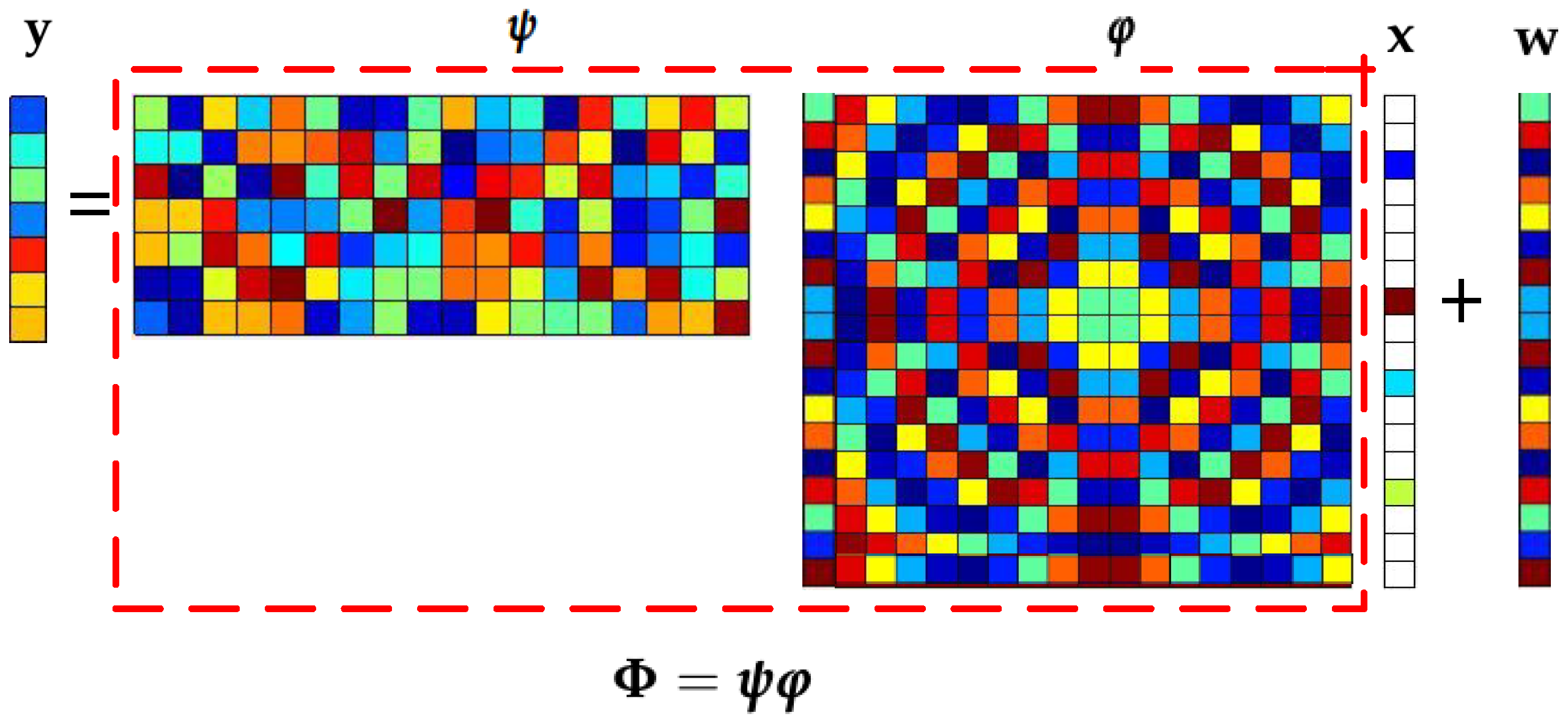
:1. Introduction
- Greedy search by using the known sparsity as a constraint;
- The relaxation method for the .
- Using sparsity as prior information;
- Using the least squares error as the iterative criterion.
2. Main Work of This Paper
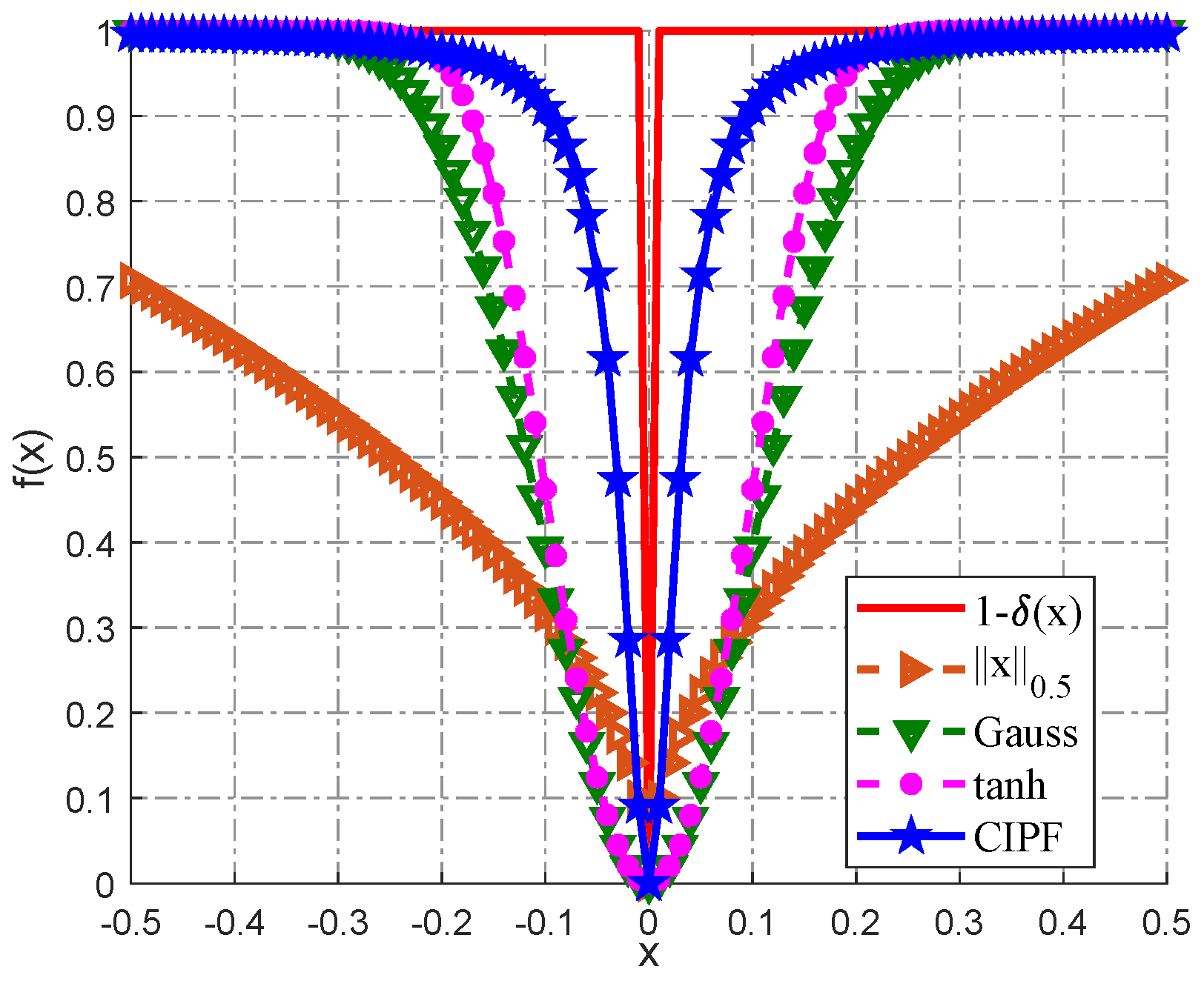
2.1. New Smoothed Function: CIPF
- (a)
- f is real analytic on for some ;
- (b)
- , , where is some constant;
- (c)
- f is convex on ;
- (d)
- ;
- (e)
- .
- It closely approximates the -norm;
- It is simpler in form than that in the Gauss and tanh function models.
2.2. New Weighted Function
- Candès et al.: ;
- Pant et al.: , is a small enough positive constant.
3. New Algorithm for CS: WReSL0
3.1. WReSL0 Algorithm and Its Steps
3.2. Selection of Parameters
3.2.1. Selection of Parameter
3.2.2. Selection of Parameter
4. Performance Simulation and Analysis
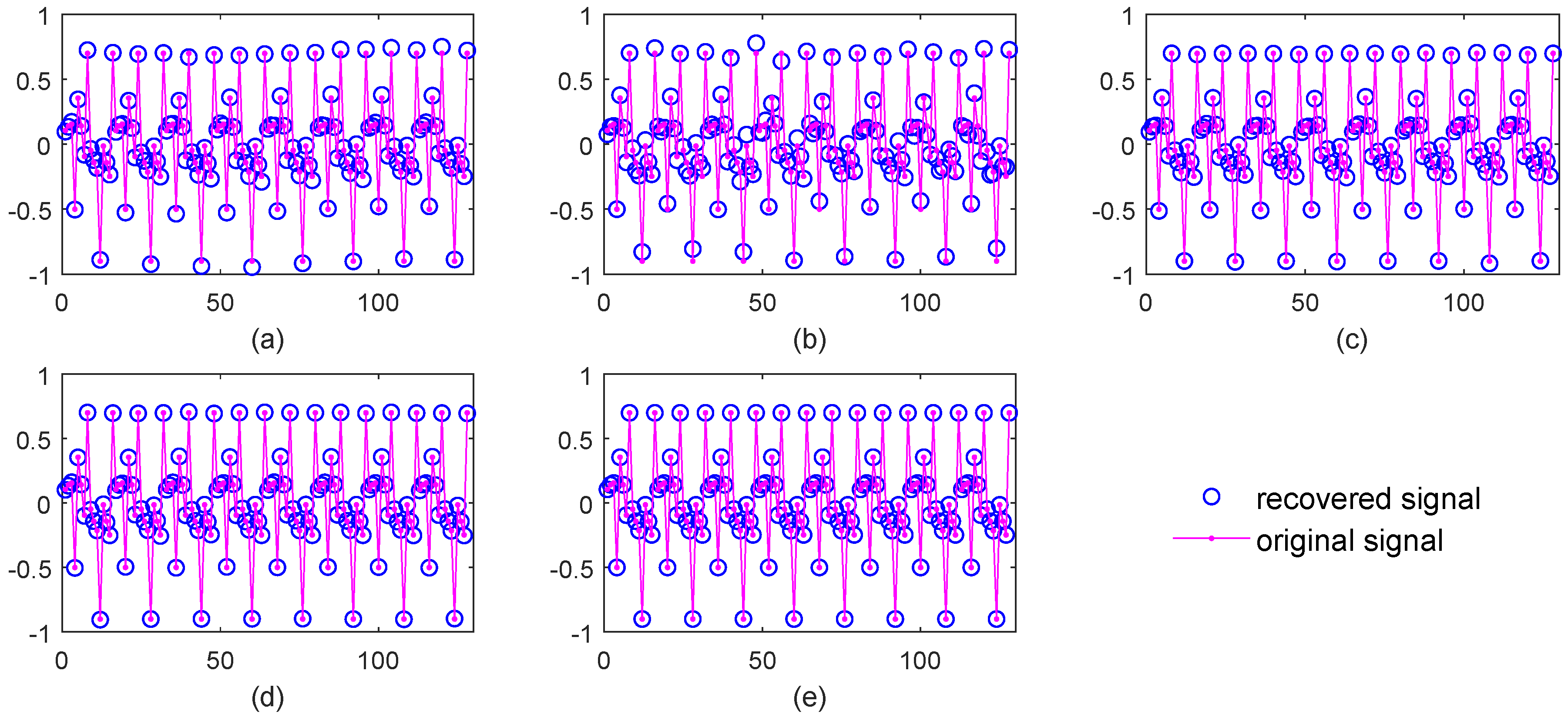
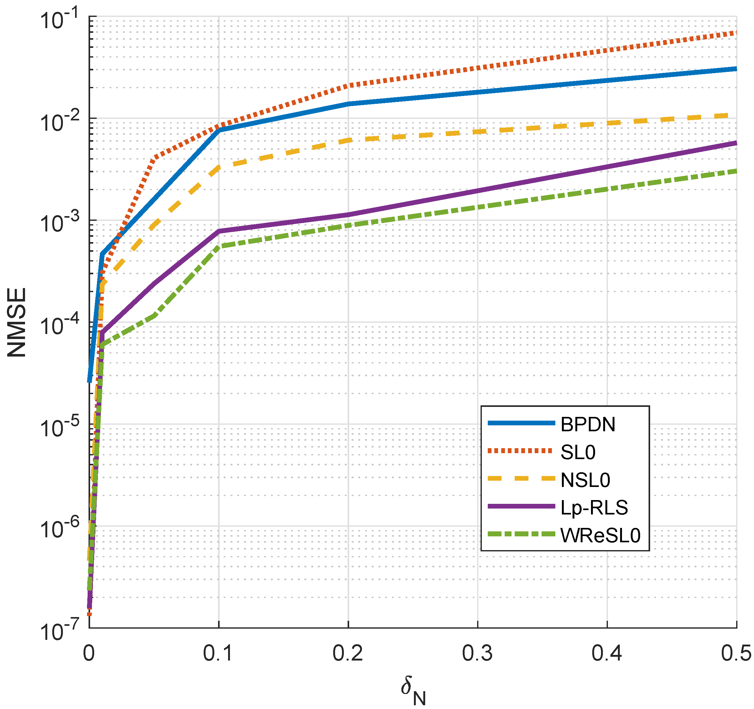
4.1. Signal Recovery Performance in the Noise Case
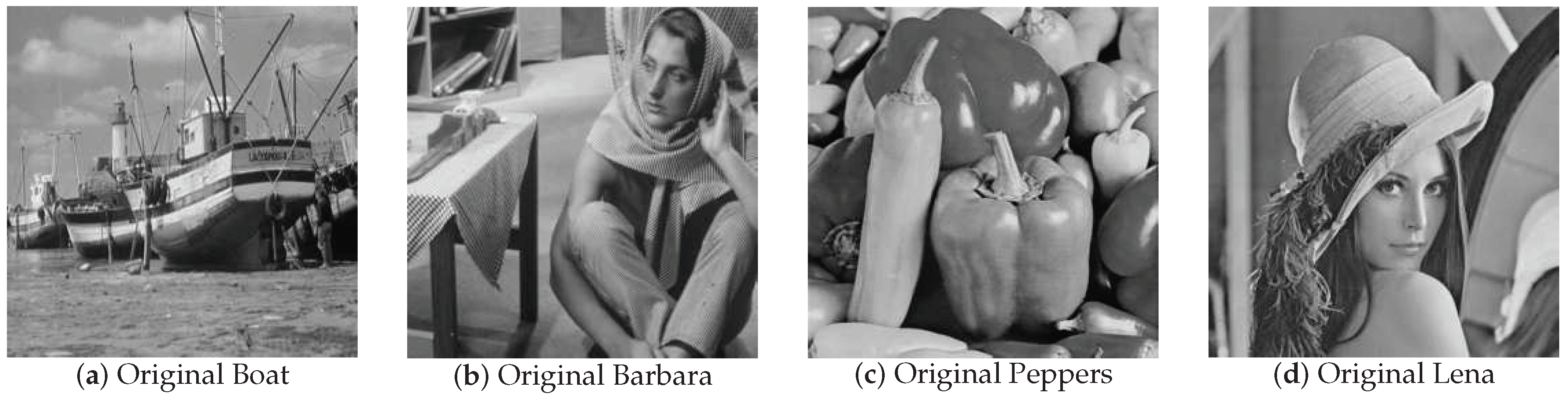
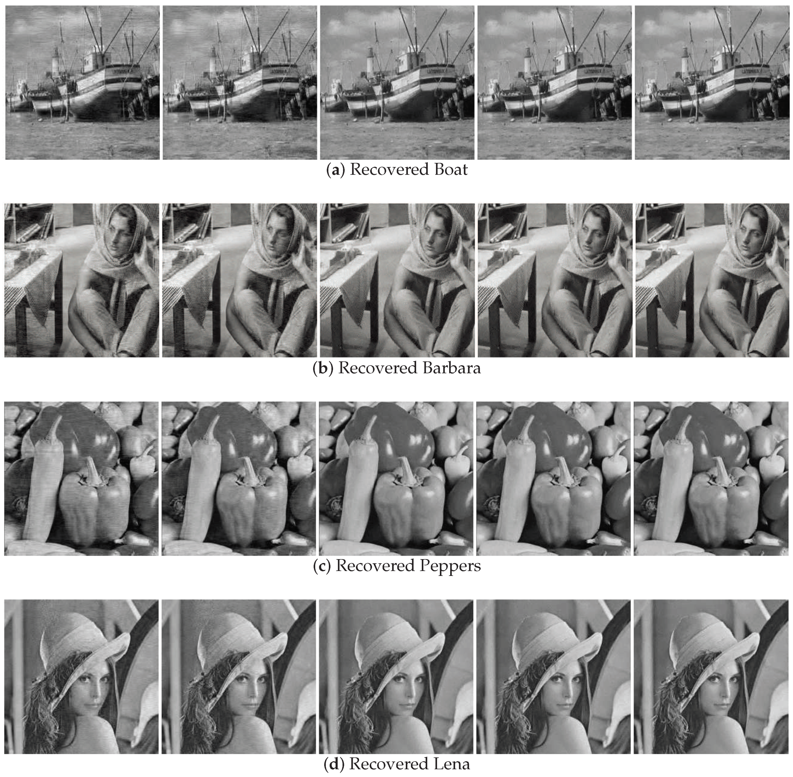
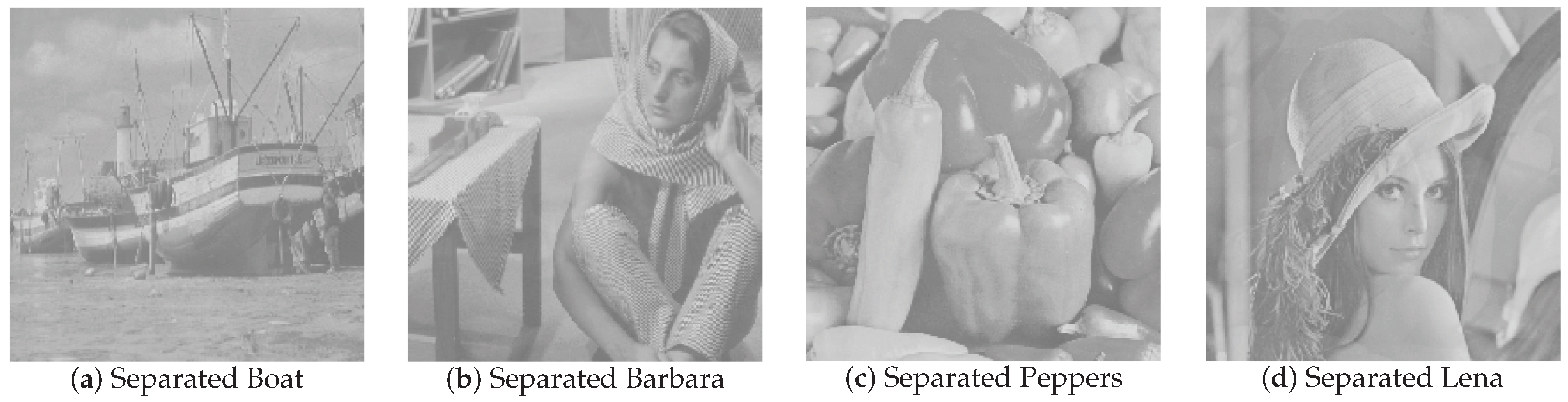
4.2. Image Recovery Performance in the Noise Case
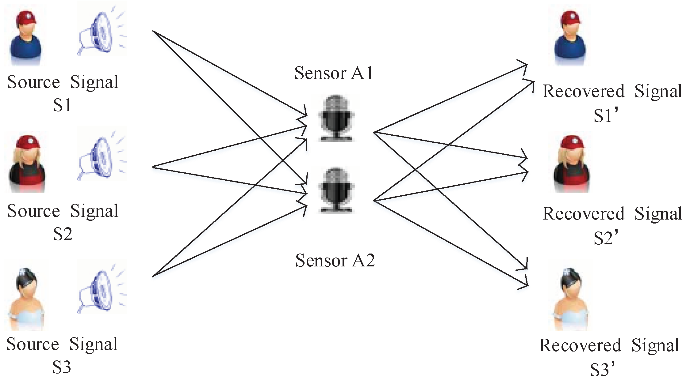
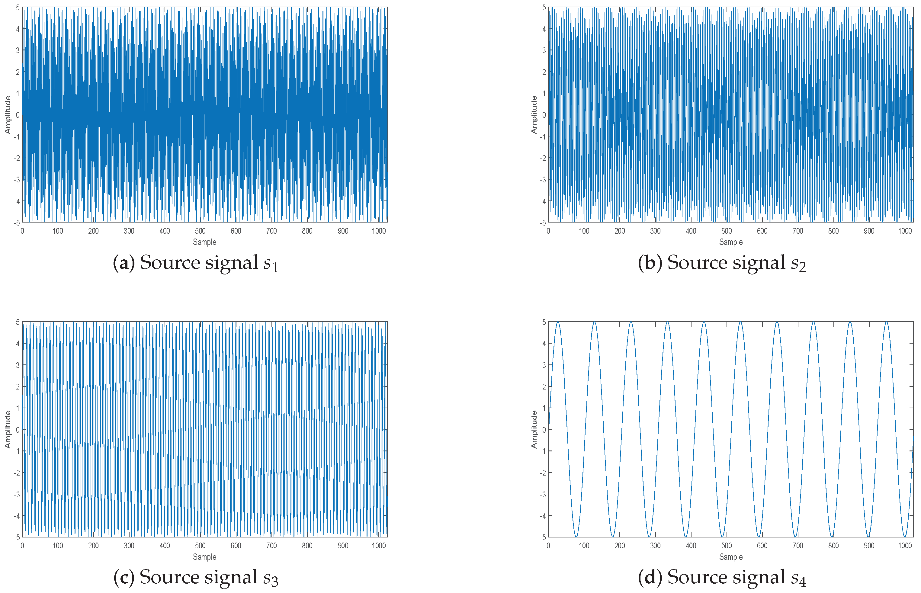
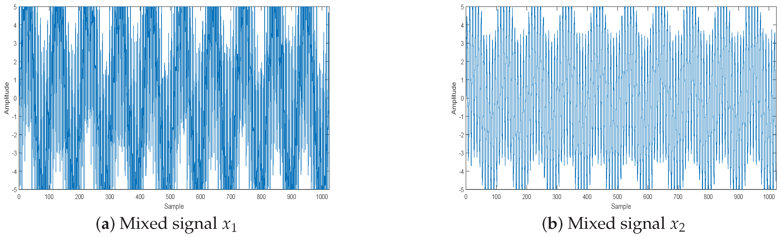
5. Application in Underdetermined Blind Source Separation
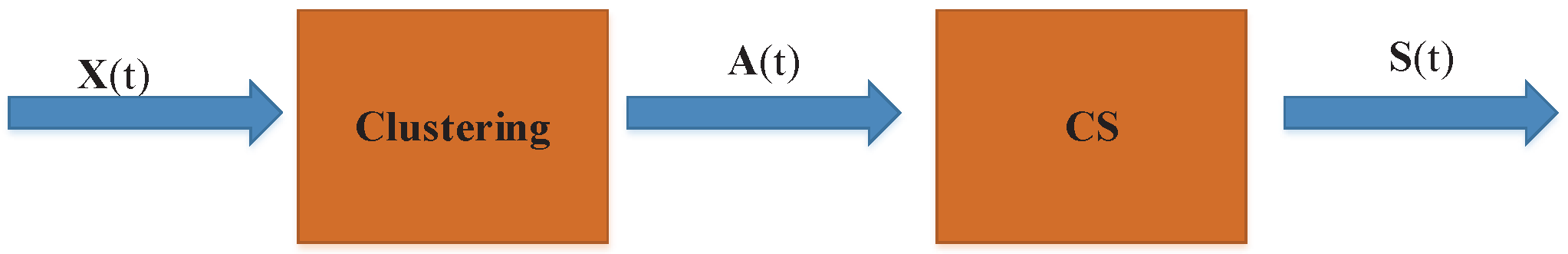
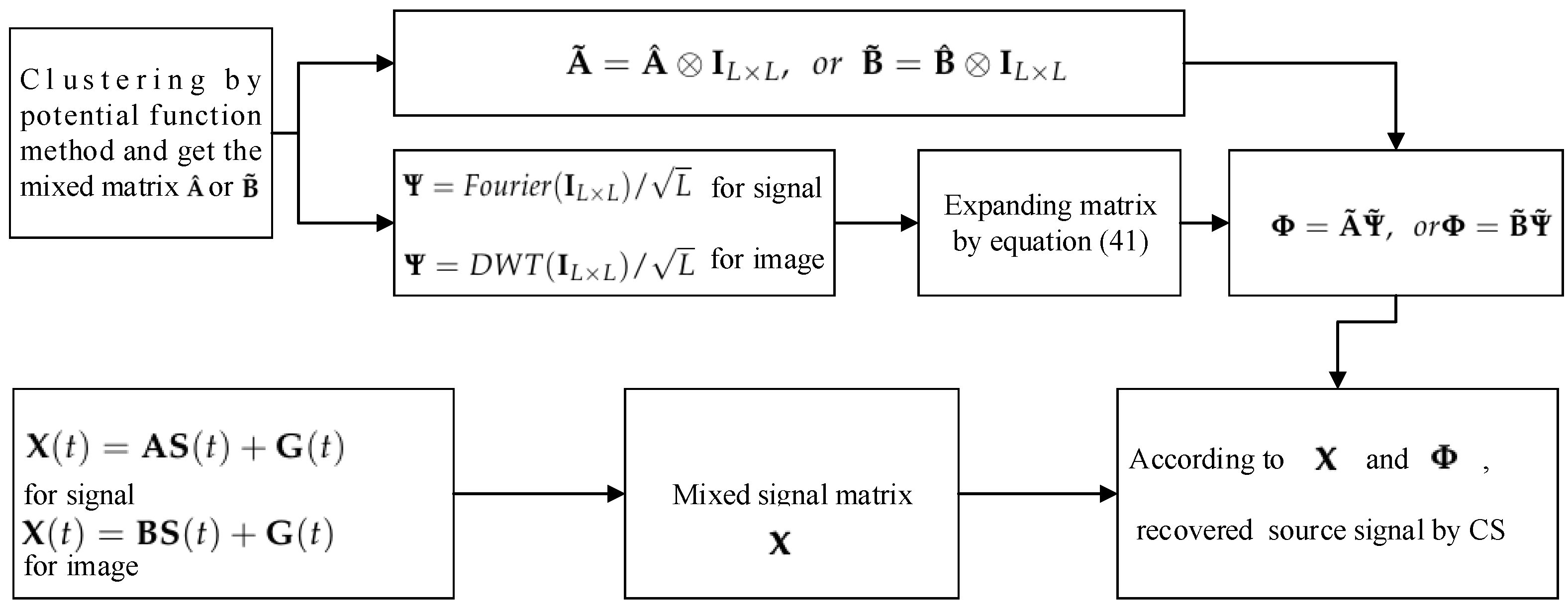
5.1. Process Analysis of CS Applied to UBSS
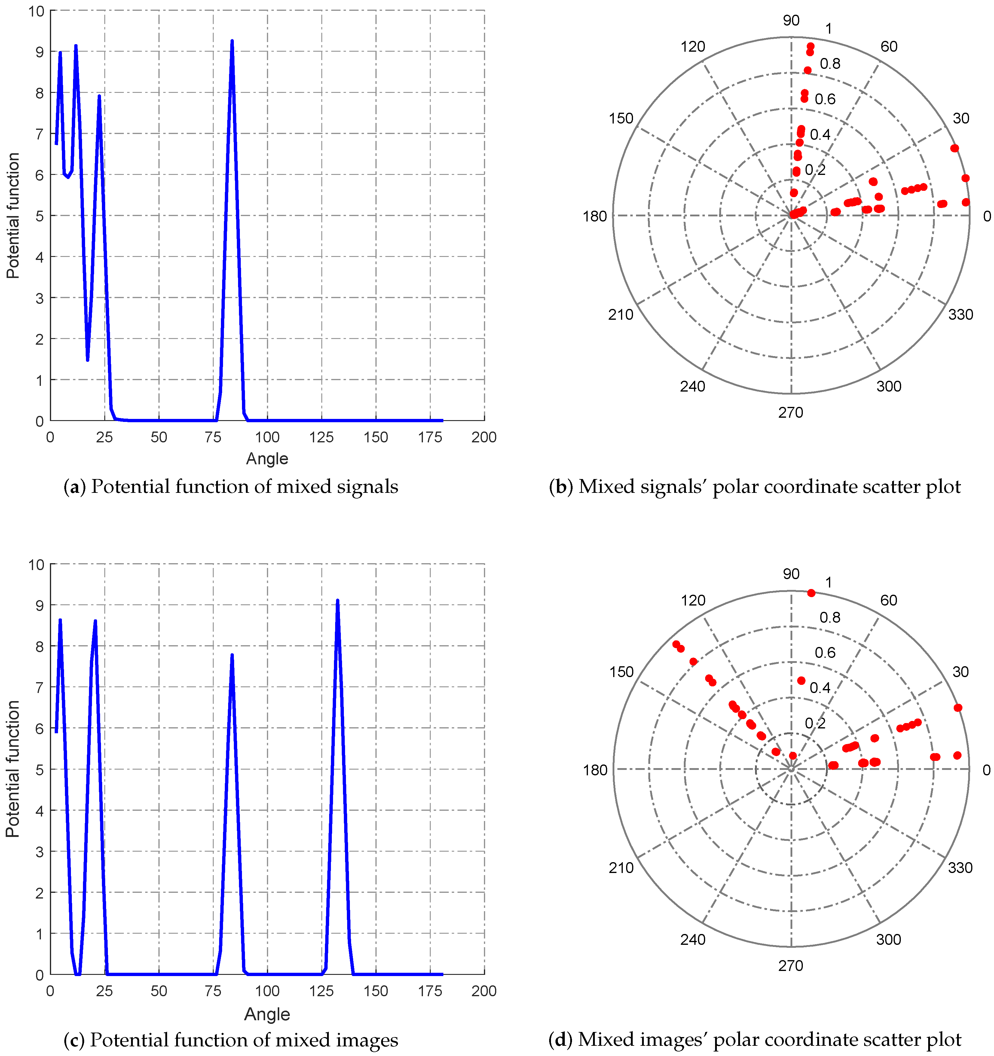
5.1.1. Solving the Mixed Matrix by the Potential Function Method
5.1.2. Using CS to Separate Source Signals
5.2. Performance Analysis of the WReSL0 Algorithm Applied to UBSS
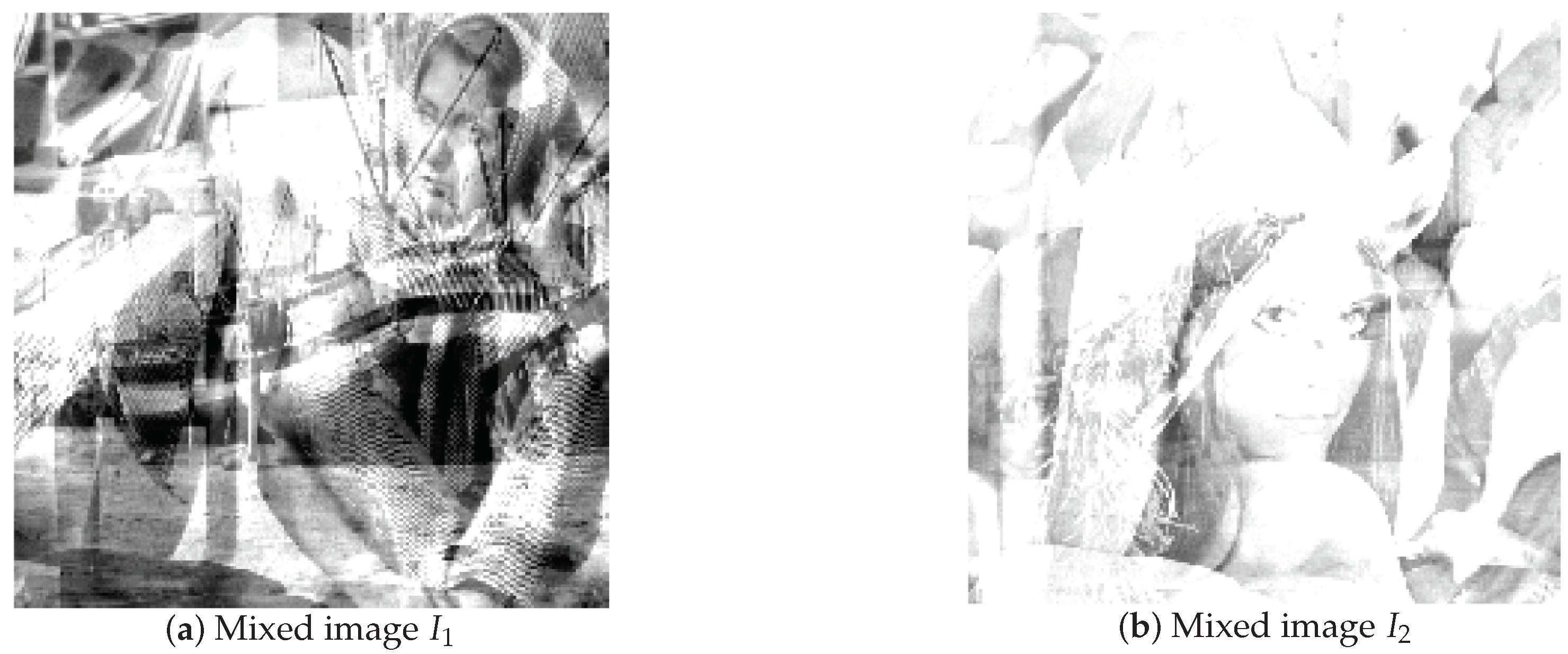
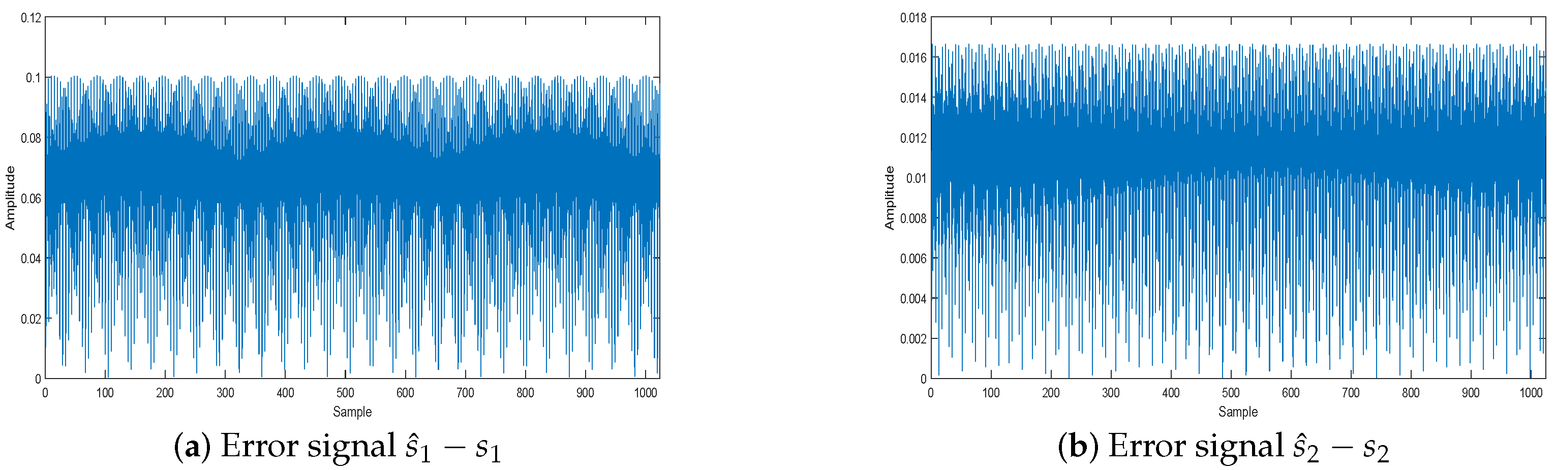
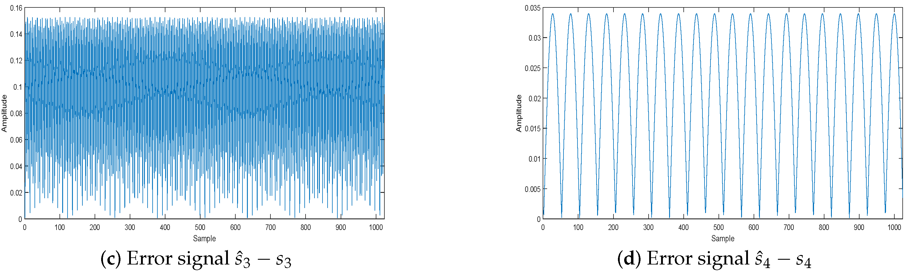
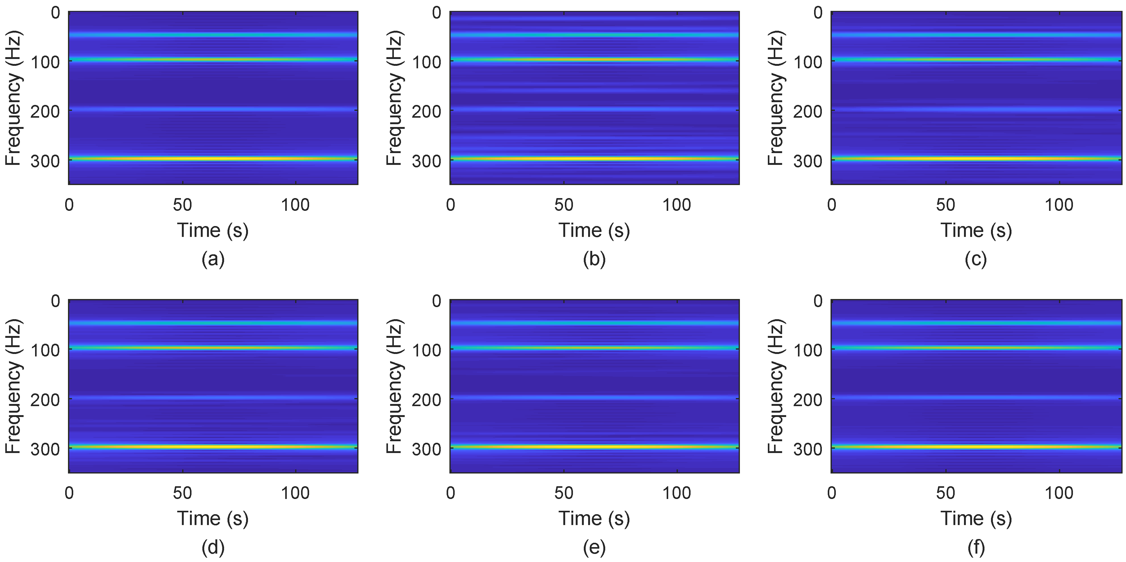
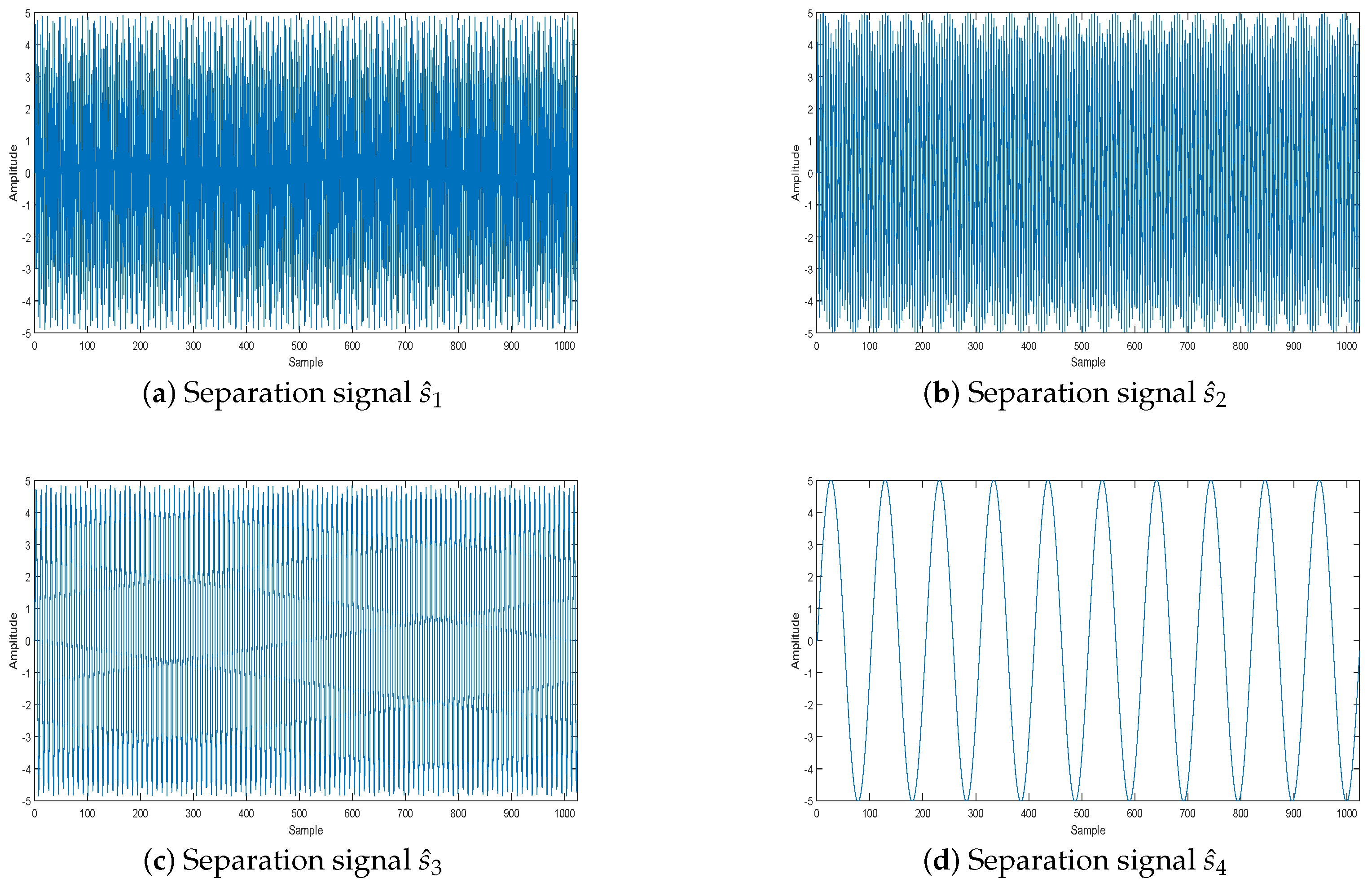
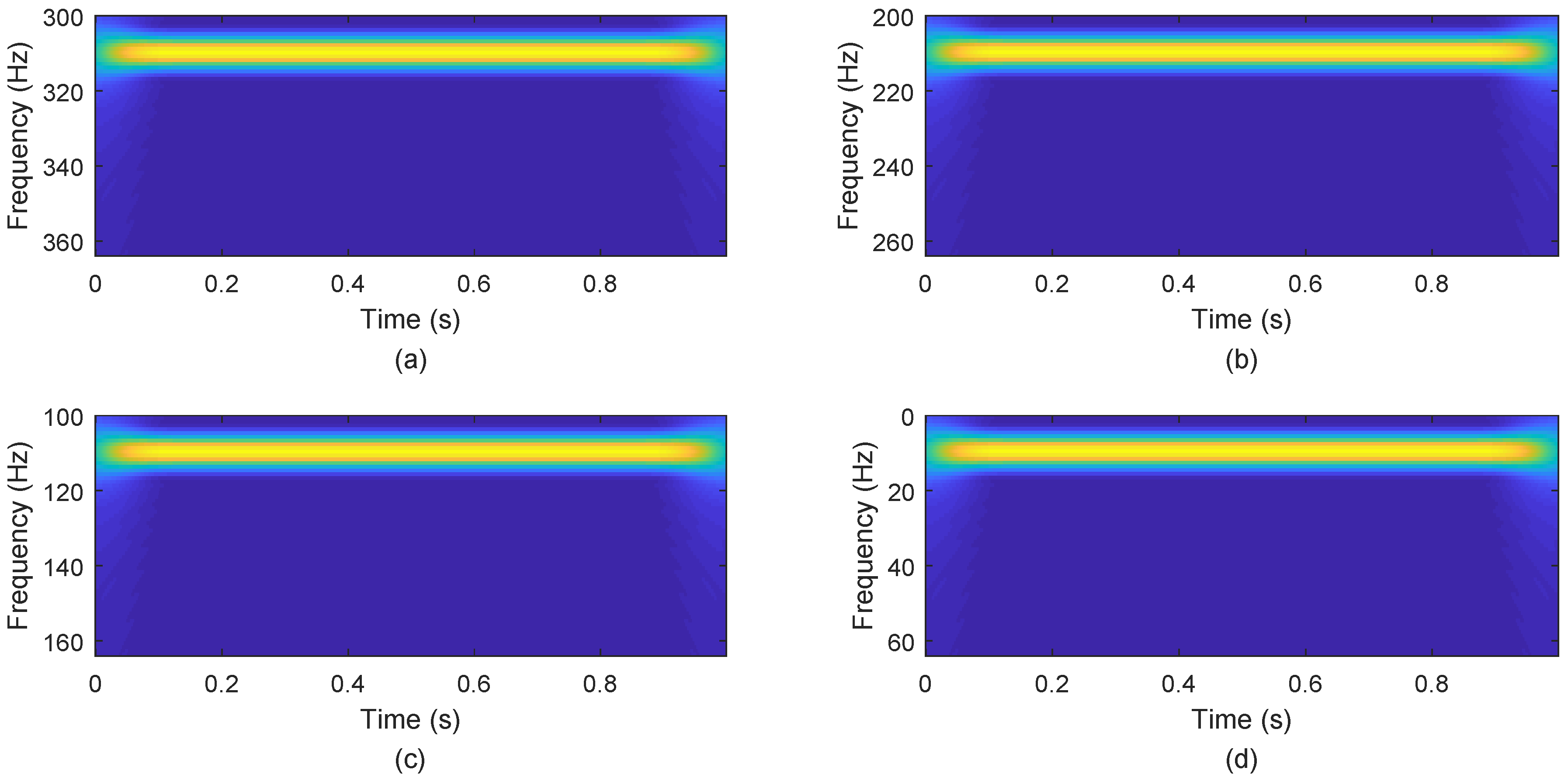
5.2.1. The Effect of the WReSL0 Algorithm Applied to UBSS
5.2.2. Performance Comparisons of the Selected Algorithms
6. Conclusions
Author Contributions
Funding
Acknowledgments
Conflicts of Interest
References
- Zhang, C.Z.; Wang, Y.; Jing, F.L. Underdetermined Blind Source Separation of Synchronous Orthogonal Frequency Hopping Signals Based on Single Source Points Detection. Sensors 2017, 17, 2074. [Google Scholar] [CrossRef]
- Zhen, L.; Peng, D.; Zhang, Y.; Xiang, Y.; Chen, P. Underdetermined blind source separation using sparse coding. IEEE Trans. Neural Netw. Learn. Syst. 2017, 99, 1–7. [Google Scholar] [CrossRef] [PubMed]
- Donoho, D.L. Compressed sensing. IEEE Trans. Inf. Theory 2006, 52, 1289–1306. [Google Scholar] [CrossRef]
- Candès, E.J.; Wakin, M.B. An introduction to compressive sampling. IEEE Signal Process. Mag. 2008, 2, 21–30. [Google Scholar] [CrossRef]
- Badeńska, A.; Błaszczyk, Ł. Compressed sensing for real measurements of quaternion signals. J. Frankl. Inst. 2017, 354, 5753–5769. [Google Scholar] [CrossRef] [Green Version]
- Candès, E.J. The restricted isometry property and its implications forcompressed sensing. C. R. Math. 2008, 910, 589–592. [Google Scholar] [CrossRef]
- Cahill, J.; Chen, X.; Wang, R. The gap between the null space property and the restricted isometry property. Linear Algebra Its Appl. 2016, 501, 363–375. [Google Scholar] [CrossRef] [Green Version]
- Huang, S.; Tran, T.D. Sparse Signal Recovery via Generalized Entropy Functions Minimization. arXiv, 2017; arXiv:1703.10556. [Google Scholar]
- Tropp, J.A.; Gilbert, A.C. Signal recovery from random measurements via orthogonal matching pursuit. IEEE Trans. Inf. Theory 2007, 12, 4655–4666. [Google Scholar] [CrossRef]
- Determe, J.F.; Louveaux, J.; Jacques, L.; Horlin, F. On the noise robustness of simultaneous orthogonal matching pursuit. IEEE Trans. Signal Process. 2016, 65, 864–875. [Google Scholar] [CrossRef]
- Donoho, D.L.; Tsaig, Y.; Starck, J.L. Sparse solution of underdetermined linear equations by stagewise orthogonal matching pursuit. IEEE Trans. Inf. Theory 2012, 2, 1094–1121. [Google Scholar] [CrossRef]
- Needell, D.; Vershynin, R. Signal recovery from incompleteand inaccurate measurements via regularized orthogonal matching pursuit. IEEE J. Sel. Top. Signal Process. 2010, 2, 310–316. [Google Scholar] [CrossRef]
- Needell, D.; Tropp, J.A. CoSaMP: Iterative signal recovery from incomplete and inaccurate samples. Commun. ACM 2010, 12, 93–100. [Google Scholar] [CrossRef]
- Jian, W.; Seokbeop, K.; Byonghyo, S. Generalized orthogonal matching pursuit. IEEE Trans. Signal Process. 2012, 12, 6202–6216. [Google Scholar] [CrossRef]
- Wang, J.; Kwon, S.; Li, P.; Shim, B. Recovery of sparse signals via generalized orthogonal matching pursuit: A new analysis. IEEE Trans. Signal Process. 2016, 64, 1076–1089. [Google Scholar] [CrossRef]
- Dai, W.; Milenkovic, O. Subspace pursuit for compressive sensing signal reconstruction. IEEE Trans. Inf. Theory 2009, 5, 2230–2249. [Google Scholar] [CrossRef]
- Goyal, P.; Singh, B. Subspace pursuit for sparse signal reconstruction in wireless sensor networks. Procedia Comput. Sci. 2018, 125, 228–233. [Google Scholar] [CrossRef]
- Liu, X.J.; Xia, S.T.; Fu, F.W. Reconstruction guarantee analysis of basis pursuit for binary measurement matrices in compressed sensing. IEEE Trans. Inf. Theory 2017, 63, 2922–2932. [Google Scholar] [CrossRef]
- Mohimani, H.; Babaie-Zadeh, M.; Jutten, C. A Fast Approach for Overcomplete Sparse Decomposition Based on Smoothed L0 Norm. IEEE Trans. Signal Process. 2009, 57, 289–301. [Google Scholar] [CrossRef]
- Zhao, R.; Lin, W.; Li, H.; Hu, S. Reconstruction algorithm for compressive sensing based on smoothed L0 norm and revised newton method. J. Comput.-Aided Des. Comput. Graph. 2012, 24, 478–484. [Google Scholar]
- Ye, X.; Zhu, W.P. Sparse channel estimation of pulse-shaping multiple-input–multiple-output orthogonal frequency division multiplexing systems with an approximate gradient L2-SL0 reconstruction algorithm. Iet Commun. 2014, 8, 1124–1131. [Google Scholar] [CrossRef]
- Nowak, R.D.; Wright, S.J. Gradient projection for sparse reconstruction: Application to compressed sensing andother inverse problems. IEEE J. Sel. Top. Signal Process. 2007, 1, 586–597. [Google Scholar]
- Long, T.; Jiao, W.; He, G. RPC estimation via ℓ1-norm-regularized least squares (L1LS). IEEE Trans. Geosci. Remote Sens. 2015, 8, 4554–4567. [Google Scholar] [CrossRef]
- Pant, J.K.; Lu, W.S.; Antoniou, A. New improved algorithms for compressive sensing based on ℓp norm. IEEE Trans. Circuits Syst. II Express Br. 2014, 3, 198–202. [Google Scholar] [CrossRef]
- Wipf, D.; Nagarajan, S. Iterative Reweighted and Methods for Finding Sparse Solutions. IEEE J. Sel. Top. Signal Process. 2016, 2, 317–329. [Google Scholar]
- Zhang, C.; Hao, D.; Hou, C.; Yin, X. A New Approach for Sparse Signal Recovery in Compressed Sensing Based on Minimizing Composite Trigonometric Function. IEEE Access 2018, 6, 44894–44904. [Google Scholar] [CrossRef]
- Candès, E.J.; Wakin, M.B.; Boyd, S.P. Enhancing sparsity by weighted L1 minimization. J. Fourier Anal. Appl. 2008, 14, 877–905. [Google Scholar] [CrossRef]
- Pant, J.K.; Lu, W.S.; Antoniou, A. Reconstruction of sparse signals by minimizing a re-weighted approximate L0-norm in the null space of the measurement matrix. In Proceedings of the IEEE International Midwest Symposium on Circuits and Systems, Seattle, WA, USA, 1–4 August 2010; pp. 430–433. [Google Scholar]
- Aggarwal, P.; Gupta, A. Accelerated fmri reconstruction using matrix completion with sparse recovery via split bregman. Neurocomputing 2016, 216, 319–330. [Google Scholar] [CrossRef]
- Chu, Y.J.; Mak, C.M. A new qr decomposition-based rls algorithm using the split bregman method for L1-regularized problems. Signal Process. 2016, 128, 303–308. [Google Scholar] [CrossRef]
- Hu, Y.; Liu, J.; Leng, C.; An, Y.; Zhang, S.; Wang, K. Lp regularization for bioluminescence tomography based on the split bregman method. Mol. Imaging Biol. 2016, 18, 1–8. [Google Scholar] [CrossRef]
- Liu, Y.; Zhan, Z.; Cai, J.F.; Guo, D.; Chen, Z.; Qu, X. Projected iterative soft-thresholding algorithm for tight frames in compressed sensing magnetic resonance imaging. IEEE Trans. Med. Imaging 2016, 35, 2130–2140. [Google Scholar] [CrossRef]
- Yang, L.; Pong, T.K.; Chen, X. Alternating direction method of multipliers for a class of nonconvex and nonsmooth problems with applications to background/foreground extraction. Mathematics 2016, 10, 74–110. [Google Scholar] [CrossRef]
- Antoniou, A.; Lu, W.S. Practical Optimization: Algorithms and Engineering Applications; Springer: New York, NY, USA, 2007. [Google Scholar]
- Samora, I.; Franca, M.J.; Schleiss, A.J.; Ramos, H.M. Simulated annealing in optimization of energy production in a water supply network. Water Resour. Manag. 2016, 30, 1533–1547. [Google Scholar] [CrossRef]
- Goldstein, T.; Studer, C. Phasemax: Convex phase retrieval via basis pursuit. IEEE Trans. Inf. Theory 2018, 64, 2675–2689. [Google Scholar] [CrossRef]
- Wei-Hong, F.U.; Ai-Li, L.I.; Li-Fen, M.A.; Huang, K.; Yan, X. Underdetermined blind separation based on potential function with estimated parameter’s decreasing sequence. Syst. Eng. Electron. 2014, 36, 619–623. [Google Scholar]
- Bofill, P.; Zibulevsky, M. Underdetermined blind source separation using sparse representations. Signal Process. 2001, 81, 2353–2362. [Google Scholar] [CrossRef] [Green Version]
- Su, J.; Tao, H.; Tao, M.; Wang, L.; Xie, J. Narrow-band interference suppression via rpca-based signal separation in time–frequency domain. IEEE J. Sel. Top. Appl. Earth Obs. Remote Sens. 2017, 99, 1–10. [Google Scholar] [CrossRef]
- Ni, J.C.; Zhang, Q.; Luo, Y.; Sun, L. Compressed sensing sar imaging based on centralized sparse representation. IEEE Sens. J. 2018, 18, 4920–4932. [Google Scholar] [CrossRef]
- Li, G.; Xiao, X.; Tang, J.T.; Li, J.; Zhu, H.J.; Zhou, C.; Yan, F.B. Near—Source noise suppression of AMT by compressive sensing and mathematical morphology filtering. Appl. Geophys. 2017, 4, 581–589. [Google Scholar] [CrossRef]


| ● Initialization: |
|---|
| (1) Set . |
| (2) Set , , and , where , and T is the maximum number of iterations. |
| ● while , do |
| (1) Let . |
| (2) Let . |
| for |
| (a) . |
| (b) |
| (3) Set . |
| ● The estimated value is . |
| Signal Length (n) | CPU Running Time (Seconds) | ||||
|---|---|---|---|---|---|
| BPDN | SL0 | NSL0 | Lp-RLS | WReSL0 | |
| 170 | 0.195 | 0.057 | 0.091 | 0.194 | 0.063 |
| 220 | 0.289 | 0.139 | 0.230 | 0.350 | 0.142 |
| 270 | 0.495 | 0.229 | 0.426 | 0.505 | 0.291 |
| 320 | 0.767 | 0.320 | 0.639 | 0.712 | 0.509 |
| 370 | 1.059 | 0.456 | 0.926 | 0.982 | 0.892 |
| 420 | 1.477 | 0.613 | 1.133 | 1.491 | 1.017 |
| 470 | 1.941 | 0.796 | 1.478 | 2.118 | 1.344 |
| 520 | 2.619 | 1.038 | 2.089 | 2.910 | 1.882 |
| Items | Barbara | Boat | ||
|---|---|---|---|---|
| PSNR (dB) | SSIM | PSNR (dB) | SSIM | |
| SL0 | 27.983 | 0.981 | 26.959 | 0.969 |
| BPDN | 28.834 | 0.984 | 27.376 | 0.971 |
| NSL0 | 31.296 | 0.991 | 31.247 | 0.988 |
| L-RLS | 31.786 | 0.992 | 31.797 | 0.989 |
| WReSL0 | 32.244 | 0.993 | 32.369 | 0.991 |
| Items | Peppers | Lena | ||
|---|---|---|---|---|
| PSNR (dB) | SSIM | PSNR (dB) | SSIM | |
| SL0 | 28.677 | 0.982 | 30.334 | 0.987 |
| BPDN | 29.542 | 0.985 | 29.875 | 0.983 |
| NSL0 | 31.373 | 0.991 | 32.639 | 0.993 |
| L-RLS | 33.757 | 0.994 | 34.051 | 0.995 |
| WReSL0 | 34.231 | 0.996 | 34.653 | 0.997 |
| Oise Intensity () | Error of (%) | ASNR (dB) | ||||
|---|---|---|---|---|---|---|
| SPM | SL0 | NSL0 | Lp-RLS | WReSL0 | ||
| 0 | 1.763 | 45.443 | 41.576 | 42.324 | 38.412 | 39.993 |
| 0.1 | 1.763 | 36.788 | 35.278 | 36.034 | 37.091 | 39.295 |
| 0.15 | 1.763 | 31.407 | 30.754 | 32.930 | 35.332 | 38.975 |
| 0.18 | 112.6 | 26.355 | 24.063 | 25.437 | 28.305 | 26.650 |
| 0.2 | 126.3 | 11.201 | 9.974 | 12.358 | 17.549 | 15.581 |
| Noise Intensity () | Error of (%) | APSNR (dB) | ||||
|---|---|---|---|---|---|---|
| SPM | SL0 | NSL0 | Lp-RLS | WReSL0 | ||
| 0 | 3.64 | 16.447 | 19.211 | 20.035 | 16.372 | 18.483 |
| 0.1 | 3.64 | 15.639 | 16.305 | 17.327 | 15.407 | 17.849 |
| 0.15 | 3.64 | 13.407 | 14.754 | 14.930 | 14.932 | 17.351 |
| 0.18 | 133.2 | 9.355 | 11.063 | 11.437 | 10.305 | 11.650 |
| 0.2 | 142.4 | 5.201 | 5.974 | 6.358 | 3.549 | 5.581 |
© 2018 by the authors. Licensee MDPI, Basel, Switzerland. This article is an open access article distributed under the terms and conditions of the Creative Commons Attribution (CC BY) license (http://creativecommons.org/licenses/by/4.0/).
Share and Cite
Wang, L.; Yin, X.; Yue, H.; Xiang, J. A Regularized Weighted Smoothed L0 Norm Minimization Method for Underdetermined Blind Source Separation. Sensors 2018, 18, 4260. https://doi.org/10.3390/s18124260
Wang L, Yin X, Yue H, Xiang J. A Regularized Weighted Smoothed L0 Norm Minimization Method for Underdetermined Blind Source Separation. Sensors. 2018; 18(12):4260. https://doi.org/10.3390/s18124260
Chicago/Turabian StyleWang, Linyu, Xiangjun Yin, Huihui Yue, and Jianhong Xiang. 2018. "A Regularized Weighted Smoothed L0 Norm Minimization Method for Underdetermined Blind Source Separation" Sensors 18, no. 12: 4260. https://doi.org/10.3390/s18124260
APA StyleWang, L., Yin, X., Yue, H., & Xiang, J. (2018). A Regularized Weighted Smoothed L0 Norm Minimization Method for Underdetermined Blind Source Separation. Sensors, 18(12), 4260. https://doi.org/10.3390/s18124260