1. Introduction
The wireless sensor networks experience problems for applications that require mobility support, such as disaster/earthquake recovery, battlefield surveillance, monitoring and handling animals, and law enforcement situations. These applications require a dynamically adoptable WSN network with mobility support to guarantee reliable communication, reliable network connectivity, low energy consumption and a longer network lifetime [
1].
Thus, it is essential to introduce a system that is energy efficient at all levels of the protocol stack. The energy efficiency and scalability of WSNs depend on the mobility variances [
2]. As a result, the lack of a robust mobility model results in performance degradation and unpredictable broken links [
3].
Furthermore, mobility plays a significant role in identifying the time-based features of network traffic in WSNs that directly affect resource provision structures and enable network designed control. It has been confirmed that high traffic load posed by a single sensor node is narrowly associated with the mobility inconsistency of that node and the spatial connection with the observed phenomenon [
4].
Bursty traffic is more likely in a scenario with high mobility variations and low spatial links. Conversely, balanced traffic is more likely when mobility discrepancy decreases and spatial correlation upsurges. These observations point out that certain mobility characteristics can produce the desired outcome in different temporal constructions of network traffic. On the other hand, mobility-based WSNs are usually preferable over static WSNs because they result in better energy efficiency, enhanced coverage, improved object tracking, and higher channel capacity [
5]. There are several WSN applications where nodes should be capable of adopting mobility, which require proper consideration [
6]. The lack of mobility support also highly distracts the routing performance in WSNs. As a result, network topology changes unpredictably and paths frequently fail, which may increase packet delay and packet loss. Moreover, the QoS provisioning at the lower layers and the transport layer relatively correlates with the presence of mobility. Otherwise, sensor nodes experience the issues of emitting, increased latency, jitter and congestion.
There are several mobility models available in the literature, all of which are particularly good candidates for ad-hoc WSNs, but their behavior in WSNs worsens QoS parameters and results in high energy consumption. For example, RWMM performs reasonably well in ad-hoc wireless networks, but is a poor candidate for WSNs due to weak choice of velocity distribution and uniform distribution [
7,
8,
9]. To overcome the shortcomings of RWMM, the nomadic community mobility model (NCM) was introduced. This model is suitable for military applications and mobile communication in conferences because nodes move randomly as a group from one location to another. However, the reference point of each node is identified based on the overall movement of the group [
10,
11]. This model consumes an excess energy when determining the location of a single node.
To handle the mobility of sink nodes, CMM was introduced. This model captures data while following a circular pathway that is based on static points. A major shortcoming of this model is that nodes must remain motionless for eight or sixteen times in each cycle. In order to extend the network lifetime, WMM, based on eight directions, was introduced [
12], but this model is specifically designed for sink nodes, but nodes have only group mobility support. Consequently, in determining the location of a single node, group nodes move and consume energy [
13]. As a result, WMM mobility model suffers due to the extra pause time, the speed of nodes, and the dependency of nodes- movement in the group causes the network performance to slow down [
14]. Furthermore, existing mobility models are fit for determining the sink mobility, but experience problems in the case of node mobility. The state-of-art in this research is to maintain QoS provisioning and prolong the network lifetime. To improve the performance of WSNs, this paper introduces the LMM. The LMM has features of handling the upward, lateral, and even downward movement. For example, a sensor node may be promoted to be a sink node, but to continue to work as a node at the same time, the node may need to take a lateral step to gain knowledge regarding other nodes for sending and receiving the data (e.g., schedules, priorities). After gaining these details, the node may then become a sink node again, this time in measuring the energy rather than distance and location. The LMM handles the limitations of existing models and makes the following contributions:
Handling the node and sink mobility concurrently.
Reducing control packets when detecting the location of nodes.
Decreasing extra pause time.
Determining the node’s distance from the previous to the current location, on variance mobility rates.
The remaining sections are organized as follows:
Section 2 gives an overview on the state of the art research.
Section 3 highlights the existing problem and mobility model formulation.
Section 4 describes the simulation setup and the analysis of results,
Section 5 gives the discussion of the results and finally
Section 6 concludes the work.
2. State of the Art Overview
There are several WSN applications such as disaster/earthquake recovery, battlefield surveillance, and monitoring bird and animal activities, which require the availability of strong mobility features. Understanding the mobility models in a realistic environment is a challenging task. In the real world, mobility is of paramount significance. Considering the behavior of the real-world entities, mobility models are categorized as synthetic or trace-based [
15]. Synthetic models scale the real-world mobile objects. However, these models are unable to show an exact behavior of movable patterns. On the other hand, trace-based models involve a large number of contestants for a longer monitoring period, but the real trajectory movement of mobile nodes is hard to capture. The above is concerning due to the deployment of emerging applications for mobility-aware environments. In particular, when sensor nodes are moving, it is challenging to maintain the QoS provisioning and prolong the network lifetime.
Many researchers have focused on deploying the mobile nodes in WSNs to extend the network lifetime and improve the performance. As a result, there are some of the interesting contributions focusing on the mobility available in the literature. However, majority of the existing contributions in mobility models use the single mobile node to gather the information from stationary nodes. Most of the existing multi-node supported mobility models focus on the mobile sensor nodes but lack the mobile-sink support. One of interesting contributions focusing on the Modified De Bruijn graph (MDBG) model is introduced to support mobile sinks [
16]. The model helps collect the data from static sensor nodes. This model aims to combine single and multi-hop communication for decreasing the end-to-end delay, but did not focus on the accuracy. Handling this issue, the extended Mobility Markov Chain model is introduced [
17] to combine the n preceding visited locations in order to improve the accuracy when determining the next predictable location. However, the model did not control the movement of individual sensor nodes. The authors in [
18] introduced a two-tier autoregressive group mobility model to handle the individual sensor nodes’ movement by using a first-tier. Furthermore, the group mobility behavior is apprehended in the second tier by using the mobility correlation of nodes. As a result, the group is acknowledged by applying the correlation index test. In addition, the model estimates the group-based mobility where representative mobility-aware node is used to calculate the mobility state of the group members. On the other hand, the two-tier autoregressive group mobility model is unable to accumulate the complete information of the clusters. In [
19], a mobility model for self-configuring mobile sensor networks is introduced to calculate the mobility patterns of mobile sensor nodes applying artificial potential functions and cluster formation. The mobility is calculated by applying two components: particle and potential field, which are based on artificial potential functions. This model lacks support for determining the mobility of individual nodes. Thus, the topology-based mobility model is proposed to support main aspects of the random waypoint mobility model and random-way-walk mobility model [
20]. The mobility model is incorporated with a lightweight medium access control protocol to achieve the objects of random walking patterns. This model handles each mobile sensor node individually, but increases the number of the control messages. The simple truncated Levy walk mobility model is introduced to capture the tendency of the people that move within predefined area of routine activities [
21]. The simple truncated Levy walk mobility model reduced the control messages by using emulation. However, the model is used for mobile ad hoc networks and delay-tolerant networks. In [
22], static sink and mobile sink are comprehensively described that collect the data by ending the locality of the sensor nodes. In the first step, performance of three different approaches is investigated in order to design and develop sink mobility models for energy efficient data gathering and delay-tolerant static wireless sensor networks. In the second step, a sensor node is randomly chosen based on the maximum number of exposed neighbor nodes. Finally, the authors recommend to use random node selection-based strategy for sink mobility models instead of keeping the track of the number of exposed neighbor nodes per node and available residual energy of the sensor node. These existing mobility models either focus on maintaining the connectivity or throughput performance. Whereas, our proposed lattice location-based mobility model concurrently determines the node and sink mobility for improving the energy efficiency and QoS provisioning. It reduces the pause time, number of control packets and node dependency. Furthermore, it also detects the node’s moving location, the distance from its previous location to its current location, and the distance from its existing location to its destination.
3. Problem Statement and Lattice Mobility Model Formulation
The limitations postured by the mobility of WSNs greatly interrupt the smooth communication process. Moreover, it is quite difficult to concurrently address the problems of node and sink mobility. The key question is how to enable WSNs to efficiently maintain QoS provisioning and extend the network lifetime with respect to imposed mobility limitations for robust disaster/earthquake salvage operations.
In a WSN, the mobility behavior in the mobile sensor node can be categorized by a two-phase process—an active and an inactive phase. During an active phase, the compressed data are transmitted to other nodes or sinks. During an inactive phase, a mobile sensor node moves to a new location, then collects and locally compresses data. To frame this mobility behavior, we introduce the LMM to control the random movement of sensor nodes over WSNs. The idea of the lattice comes from a moderately ordered set in which every pair of elements is based on a supremum (known as a join or least upper bound) and an infimum (known as a meet or greatest lower bound). For example, the network ‘n’ consists of different regions and supremum can be considered as a subset ‘’ or a network region-1 ‘n’, but it could be partially ordered set of another region ‘R’. Thus, nodes in ‘’ are referred to as least element in R. The nodes in another region ‘R’ are greater than or equal to all the existing elements of ‘’. As a result, supremum is also referred to as the least upper bound (LUB).
On other hand, infimum is the subset ‘
’ or a network region-2 that is partially ordered set of another region ‘
R’, but the nodes of ‘
’ are greatest elements in ‘R’ that are less than or equal to all elements of ‘
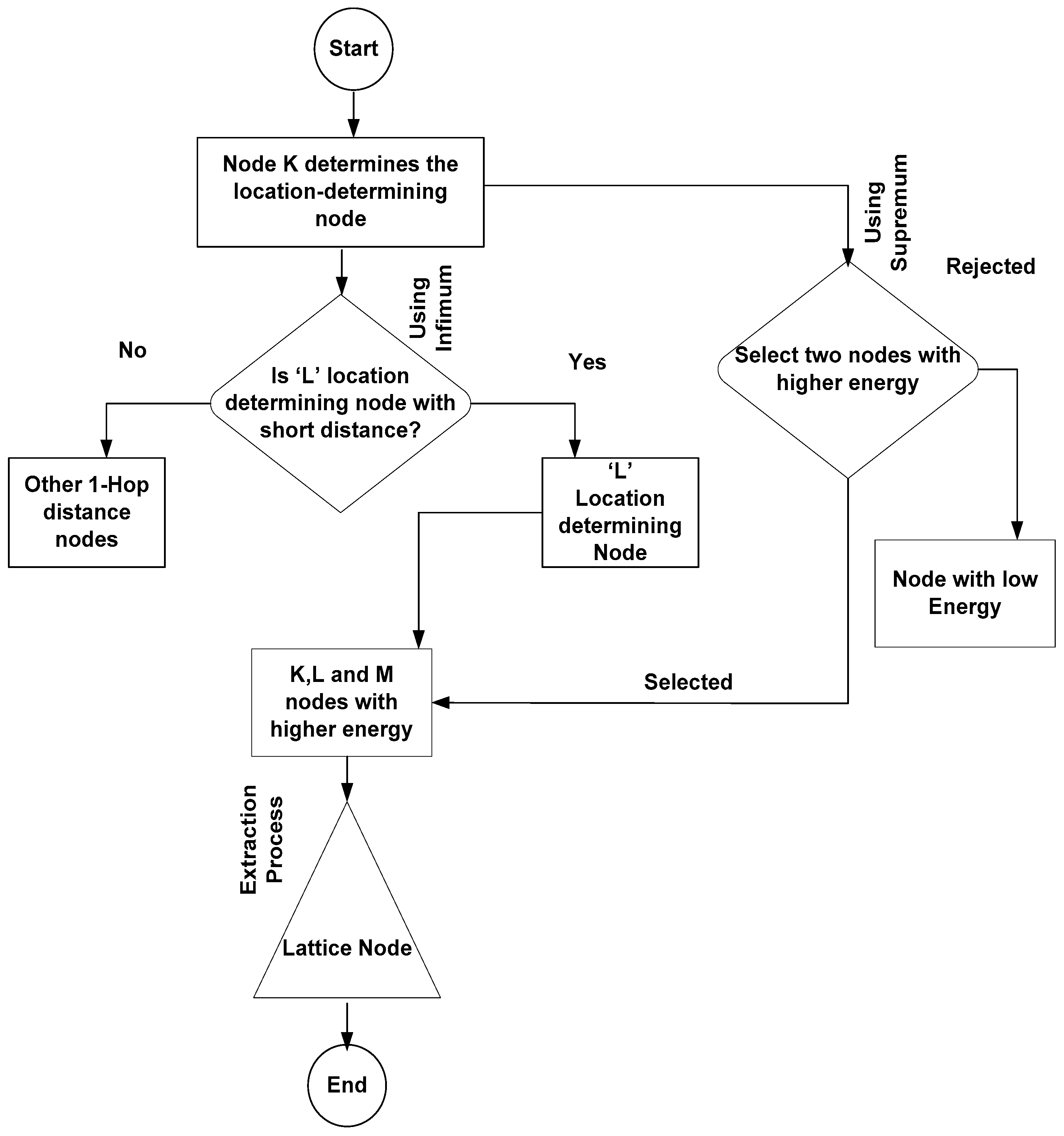
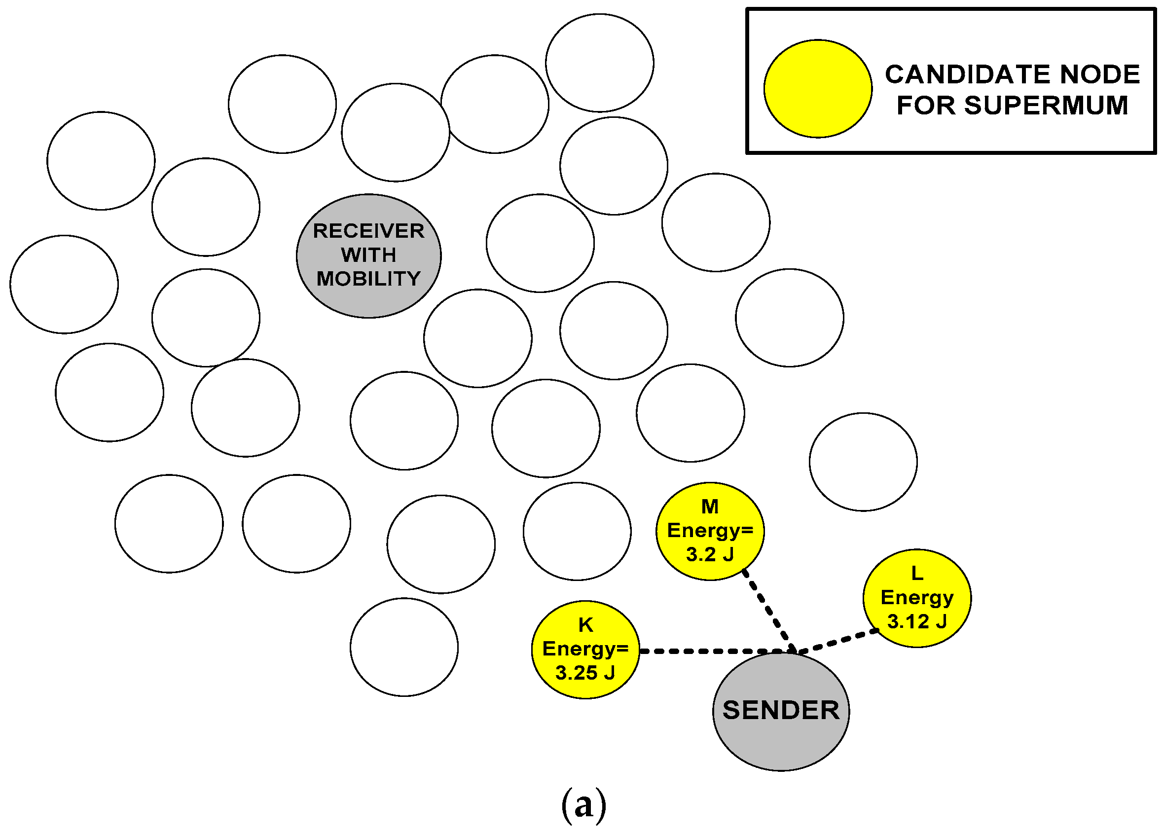
’. As a result, infimum is referred to as greatest lower bound (GLB). Thus, an idea of supremum and infimum is applied in the LMM, which helps the sensor nodes maintain connectivity and choose the node with more energy and the shortest distance during the communication. We choose the specific node for targeting the mobility-aware node based on the least distance and high residual energy using the concept of infimum and supremum, as depicted in
Figure 1. We formulate the problem using supremum and infimum. The supremum is used to represent and sample the maximum energy of senor node in the region ‘
R’ and infimum is used for determining the shortest distance of node available at 1-hop neighborhood. Let ‘
K’ be a sensor node that wants to find the location and distance of communicating node. Thus, node ‘
K’ uses infimum features to determine the 1-hop neighbor distance node that is called as the location-determining node ‘
L’. ‘
L’ is the closest node to ‘
K’ in the region ‘
R’ in the network ‘
N’. In addition, we initially pick three nodes, including ‘
K’ in the same region with maximum energy. These nodes are ‘
K’, ‘
L’ and ‘
M’ with the highest residual energy. The nodes are picked using supremum features for determining the highest energy available in the node at 1-hop neighbor distance. Based on infimum and supremum, the next node is selected to be responsible for forwarding the data and finding the location of desired destination node explained in
Figure 1.
The chosen node is called a lattice node.
Figure 2 gives a graphical representation of determining the lattice node.
In
Figure 2b, the final lattice node is the one that satisfies both conditions of supremum and infimum. If the sensor node ‘
K’ is already proved with maximum energy (supremum), then this claim can furthermore be satisfied using Theorem 1.
Theorem 1. Every nonempty search of ‘K’ node with below infimum and above supremum in the region ‘R’ is bounded.
Proof. This theorem provides the foundation for many existence results in realistic scenarios and studies. For example, once we validate that a sensor node is bounded from above, then we may prove the existence of the supremum without determining its value.
The infimum and supremum sensor node is the lattice node in the region ‘R’, which is unique, if it exists. Additionally, if both the supremum and infimum exist, then Rinfmum ≤ RSupmum. □
Proof. Assume that a sensor node ‘K’ is the supremum in the region ‘R’. Then K ≥ γ; thus, a sensor node ‘K’ is the upper bound in the region ‘R’. Similarly, if ‘K’ is the infimum sensor node in the region ‘R’, then K ≤ γ. Thus, ‘K’ is the greatest lower bound in the region ‘R’. It can be expressed as follows:
If K ≥ γ, then K = γ.
If Rinfmum and RSupmum exist, then the region ‘R’ is nonempty. Thus, select ‘K’ sensor node that is the nearest node with the highest residual energy. It can be written as:
K ∈ R, &Rinfmum ≤ K ≤ RSupmum.
Rinfmum and RSupmum are the greatest lower bound and upper bound respectively in the region ‘R’. It follows that Rinfmum ≤ RSupmum.
If RSupmum ∈ R, then it is represented as Rhigh and called the highest residual energy of the node ‘K’ in region ‘R.’ If Rinfmum ∈ R, then it is represented as Rlow and called the shortest distance of node ‘K’ from location-determining node ‘L’ in the region ‘R’. □
Based on the concept of infimum and supremum, LMM searches for the unique node with the highest residual energy and the shortest distance from the source node to the destination node.
The idea of infimum and supremum is applied with LMM to support three types of mobility patterns: dynamic medium mobility patterns, walking mobility patterns, and vehicular mobility patterns. Dynamic medium mobility patterns are used when the sensor nodes are in a medium (e.g., wind, water, or other fluid) and typically supports two or three dimensions. Walking mobility patterns are suitable for people; movements in these patterns are two dimensional. These patterns are characterized by restricted speeds, a chaotic nature, and obstacle avoidance. Vehicular mobility patterns support vehicles that are equipped with sensor nodes. The vehicles communicate by exchanging traffic conditions with each other. The movement of the vehicle is measured in only one direction.
Theorem 2. The greatest lower bound is constructed on the infimum. Let V = (a, t) be the speed of the mobile sensor node at the given time ‘t’ and at the location
Proof. In the greatest lower bound,
D = (
a,
t) is the node distribution along the direction ‘∆
di’. Each sensor node has three nearest neighbor nodes as:
where ‘
R’ is the region of the network. Thus, different direction ‘∆
di’ of neighbor node ‘
a’ in the region ‘
R’ can be defined as follows:
Greatest lower bound (Infimum) can be governed by following equation:
where ‘
’ is the distribution of the nodes that can be predicted by the value of
; we set
to be an average speed of
where ‘
i’ indicates the number of the mobile sensor nodes having an average speed.
The greatest lower bound requires that speed of mobile sensor node is measured during the progression. Mathematically, it entails that the summation of the left-hand side of Equation (3) over all three neighborhoods must be equal to 1:
Substituting Equation (5) into Equation (4), we get:
□
Thus, we summarize the result of the theorem based on the greatest lower bound (infimum) in the algorithm given as:
| Algorithm 1: The greatest lower bound (Infimum). |
(a). For all neighbor nodes
(b). For each neighbor node
(c). For each border node
Here, boarder node functions as head node to collect the data from other nodes that are within reach.
(d). Update the speed for all moving nodes
|
The goal of this contribution is to focus on the walking mobility patterns because no existing mobility model supports walking patterns well. Hence, RWMM and the group mobility model have few capable features that can be modified to support many scenarios [
23]. However, both are closer to ad-hoc and wireless networks than WSNs. LMM helps increase throughput, increase energy efficiency and reduce latency. Let us define how to use LMM in region based WSNs to handle walking mobility patterns:
Let ‘
K’ be a sensor node that reaches location ‘
L’. The probability of determining the location ‘
PK (
L)’ of the sensor node can be defined as:
Equation (7) shows the number of hops from originating node to destination node for determining the location of the desired node.
Assume that the sensor nodes in the lattice are periodic with a periodic location ‘
L’. Then no boundary condition exists, so the probability ‘
’ of determining the location of the sensor node can be calculated using the following recurrence formula:
where
is the probability of the sensor node when it moves from location ‘
L’ to location ‘Ĺ’. We introduce a generating function for the moving sensor node as follows:
where ‘
’ is the trajectory of the sensor node and ‘
’ is the state of the node in WSNs.
We express the case in which the sensor node starts moving from the origin to another destination as
where
is the Kronecker delta.
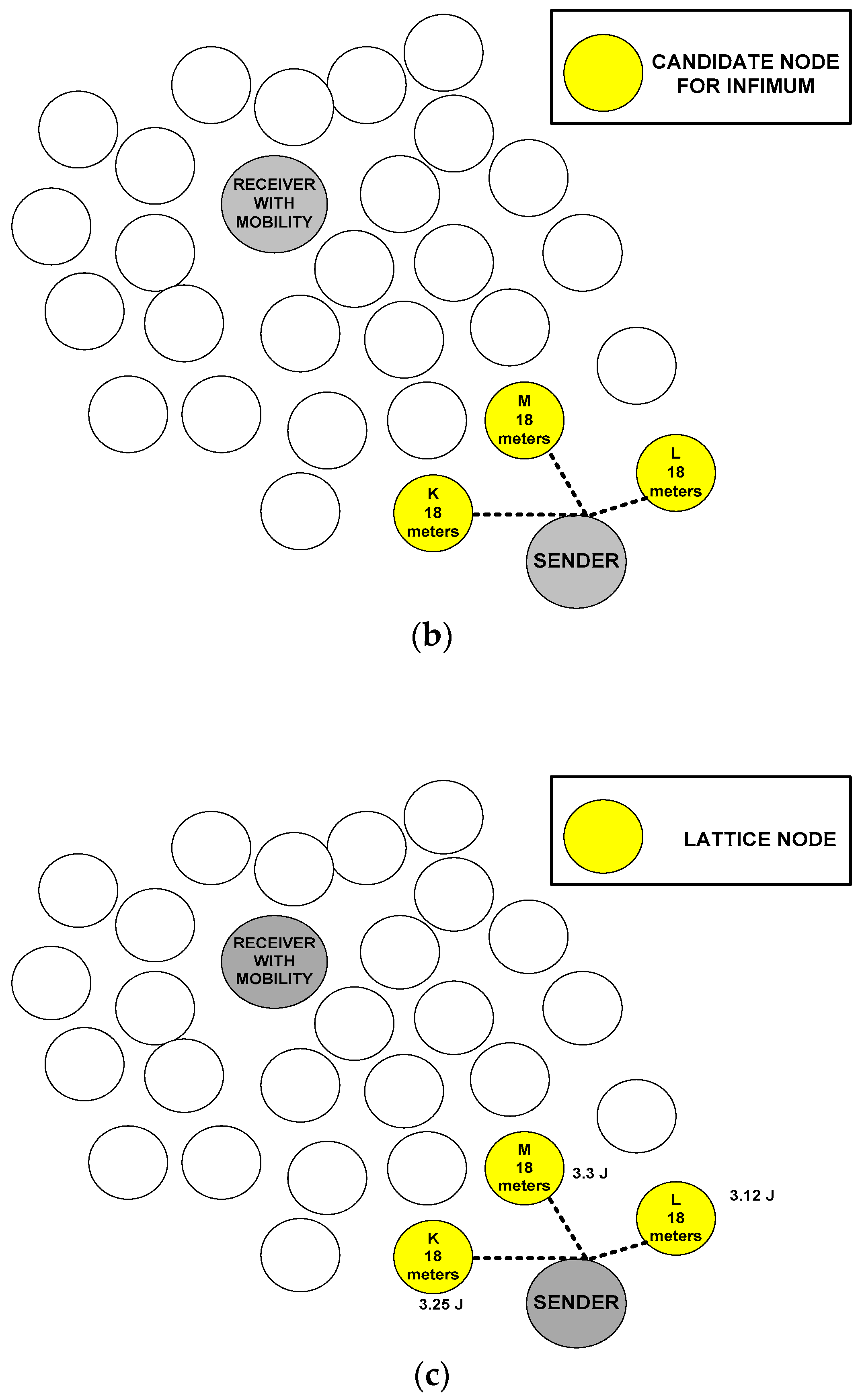
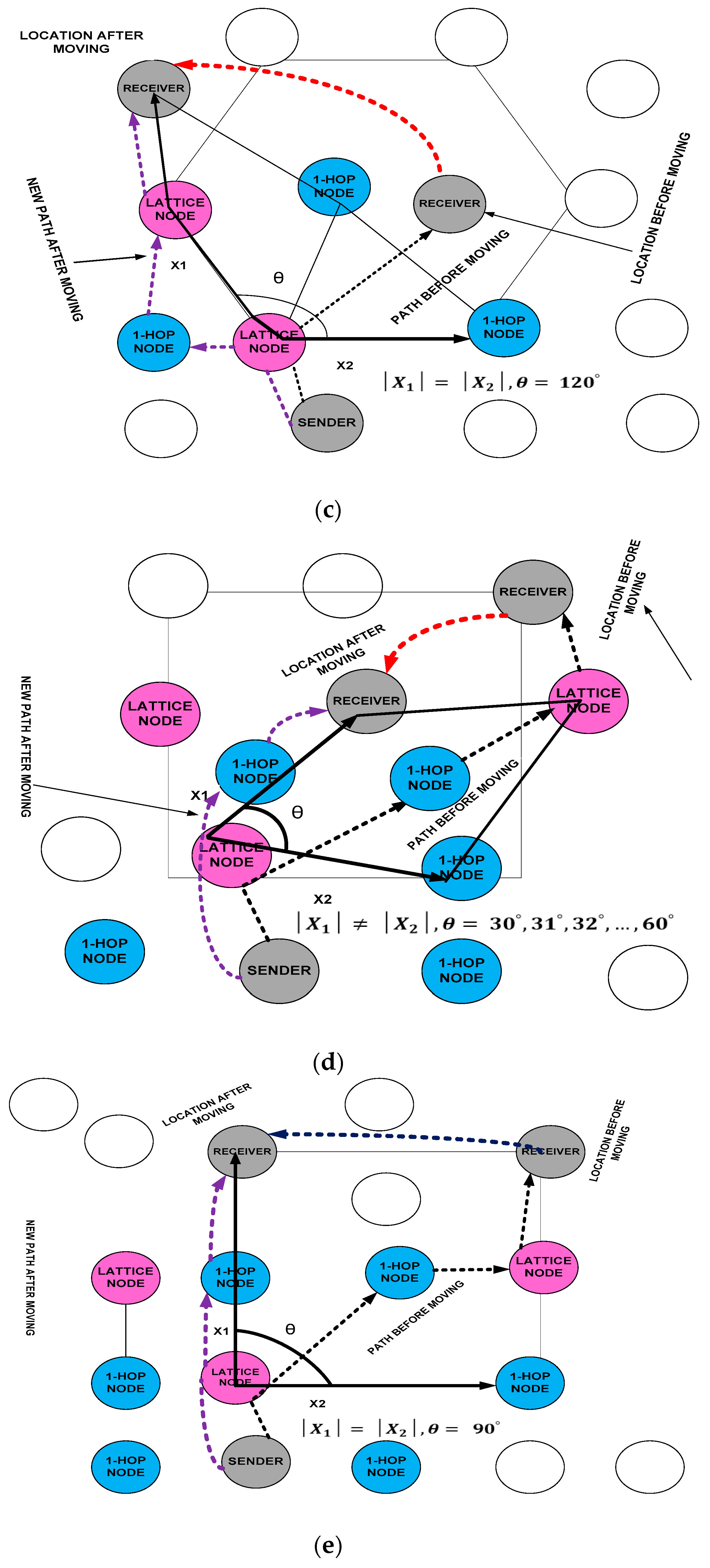
We measure the walking patterns in two dimensions, which involve five types of Bravais lattices: rectangular, oblique, hexagonal, rhombic, and square. These five Bravais lattices help determine the location of a sensor node. We apply the Fourier transform to Equation (10) to determine the accurate location of the moving sensor node. In the case of the rectangular Bravais lattice, the new location of the mobile sensor node is depicted in
Figure 3a and obtained by multiplying both sides by
and adding over
L:
where
: Lattice points on the cell corners;
: The number of dimensions
In the rectangular lattice, the node moves to the new location and creates a angle from the distance of lattice node, but does not meet the x-axis and y-axis coordinate points.
The oblique is another type of Bravais lattice that helps determine the location of mobile sensor node when it creates a trajectory smaller than . Accordingly, the new location of the moving sensor node is obtained slightly differently.
Its curve is depicted in
Figure 3b and obtained by:
The hexagonal Bravais lattice is used to determine the location of a mobile sensor node when the trajectory at the new location is exactly
. Thus, the new location of a moving sensor node is obtained by applying the Fourier inverse of
. The location of a mobile sensor node is depicted in
Figure 3c.
The rhombic is the type of Bravais lattice that can be used to find the location of a mobile sensor node when its trajectory is between
and
. Hence, the new location of mobile sensor node is obtained by using the following integrands, and the trajectory of the mobile sensor node is depicted in
Figure 3d:
The last type of two dimensional Bravais lattices is the square, which can be used to locate a mobile sensor node when its trajectory is larger than
and it satisfies the
x-axis and
y-axis coordinate points. Therefore, the trajectory of the mobile sensor node is depicted in
Figure 3e and its location is obtained as:
The transition probability ‘
T(
L)’ is used to determine the distance from the original location of the moving node to its current location using the lattice structure. A simple cubic lattice has the following property:
Therefore, we can determine the exact current distance to the sensor node as:
Equation (23) provides the actual distance between the original location of the moving sensor node and its current location. Let us now find the distance of the moving node from its current location to the final destination. We assume that the final distance is
, so
. Therefore:
where
.
The detail of used notations and descriptions is given in
Table 1.
Thus, the total energy ‘
’ consumed in updating the locations
of the sink nodes and the cost for each complete cycle (Even-monitoring process)
used in [
23] can be given by:
Equation (26) denotes the energy consumed for the location update:
Equation (27) shows the consumed energy for synchronization:
Equation (28) shows the consumed energy for receiving and forwarding the data to the next node:
By combing the Equations (26) and (29), we get the total energy consumed for updating the location and each complete cycle as given by:
This model helps accurately determine the moving location, the distance from the original location of the sensor node to the current location. Additionally, it reduces control packets by applying the optimized data frame format model approach discussed in [
23], energy consumption and end-to-end delay. The mobile sensor nodes in LMM sense the event from the target location and transfer the generated events to the base station. If any sensor node moves from its original position, another node fills the gap. The location of the moving node is determined to manage the data transmission rate.
The lattice provides scalability to WSNs because the locations and distances of the moving sensor nodes are easily determined to control the mobility. The LMM is suitable for single-hop destinations, but its performance on multi-hop destinations has not been tested. Moreover, multiple hops on the path create nonlinearities in the WSN. Before a packet can be transmitted, a node should wait for the node of the next hop to wake up. The packet is held for a variable amount of time on every path. This feature creates uncertainty for several types of WSN applications, especially surveillance and military applications.
The LMM is a memory less model because WSNs have sensor nodes with minimum memory and power. The lower energy consumption for mobility helps gather additional data due to a longer network life. We focus on other lower-memory mobility models, including the geographic based CMM, WMM, and RWMM. The performances of these mobility models are compared in the realistic scenario of an earthquake, which is simulated in the next section.
4. Simulation Setup and Analysis of Results
We simulate LMM using OMNet++ [
24]. The network contains 500 sensor nodes that are randomly deployed over a 1600 × 1600 square meter field. Initially, the border node remains in a corner of each region and movable sensor nodes are placed at the corners of the regions. When the simulation begins, the mobile sensor nodes move back and forth in the network regions. Each simulation run lasts for 14 min, and three mobility models are tested: CMM, WMM, and RWMM. We use the pheromone termite routing protocol to handle the packet generation rate and pheromone sensitivity used in [
25].
At the transport layer, packet re-ordering is a major issue, particularly for multimedia contents [
26], so we use Reliable Multi Segment Transport protocol (RMST) [
27] to help re-order the packet, which guarantees consistent pre-packet delivery for different packet types and enables faster recovery in case of packet loss. The packet size is set to 128 bytes for file transfer and 512 bytes for video, audio, and image transfer. We also consider a sensor application module with a constant bit-rate source that maintains QoS requirements. The contending algorithms CMM, WMM, and RWMM have comparable accuracy and tune our proposed LMM algorithm to have the similar accuracy in order to compare the performance. The detailed simulation parameters are presented in
Table 2.
We obtained several results, but used the following metrics to demonstrate the performance of the LMM in the WSN:
- ▪
Average delay and average power consumption
- ▪
The times taken by the sensor nodes to reach different positions using the LMM, CMM, RWMM, and WMM at fixed and variable rates of motion.
- ▪
The drop rates using the LMM, CMM, RWMM, and WMM at different rates of motion.
- ▪
The residual energy of the nodes and border node after changing the locations using the LMM, CMM, RWMM, and WMM.
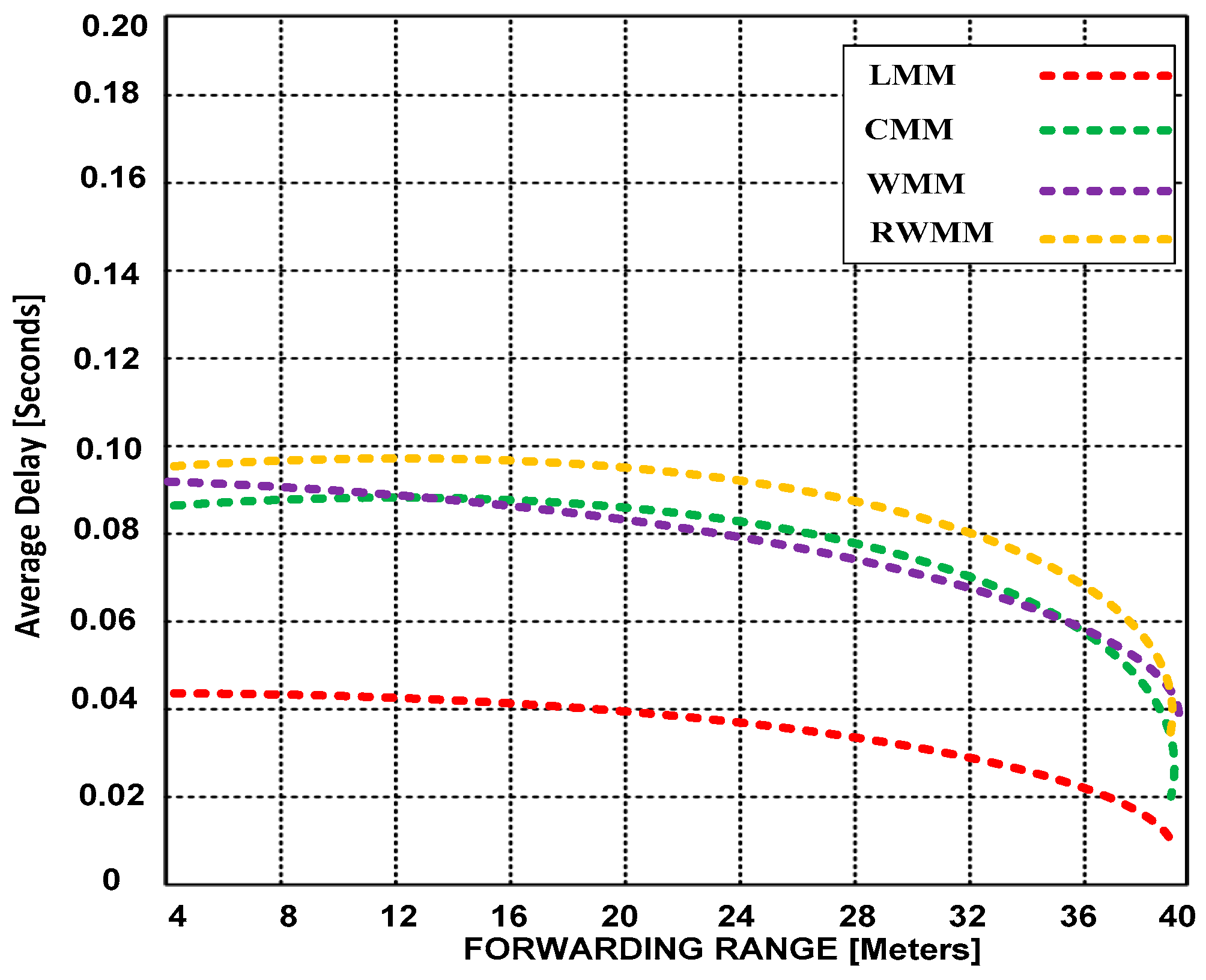
(A) Average delay and average power consumption
In
Figure 4 and
Figure 5, we show the average power consumption based on increased event range and forwarding range. The sensor node within an event area reports to the border node in each region. The event area is centered at (300, 300) meters. The figures show the simulation runs for the high moderate traffic rate. The mobility is set to 50% and an event range is 25 and 50 m around the center in
Figure 4 and
Figure 5, respectively. There are 200 sensor nodes, which participate in the event and use 42 sources (activities performed in each event).
In
Figure 4 and
Figure 5, we demonstrate that in the situation of high moderate traffic rate, which is now common in WSNs due to the emergence of new mobility based applications, reducing end-to-end delay is of paramount significance for obtaining improved throughput. Thus, we validate that end-to-end delay can be reduced by extending the forwarding range. This is a significant trade-off that has not been investigated until now. In addition, we have validated that LMM outperforms CMM, WMM and RWMM in walking mobility patterns. Furthermore, RWMM performs poorly in reduced and extended forwarding range.
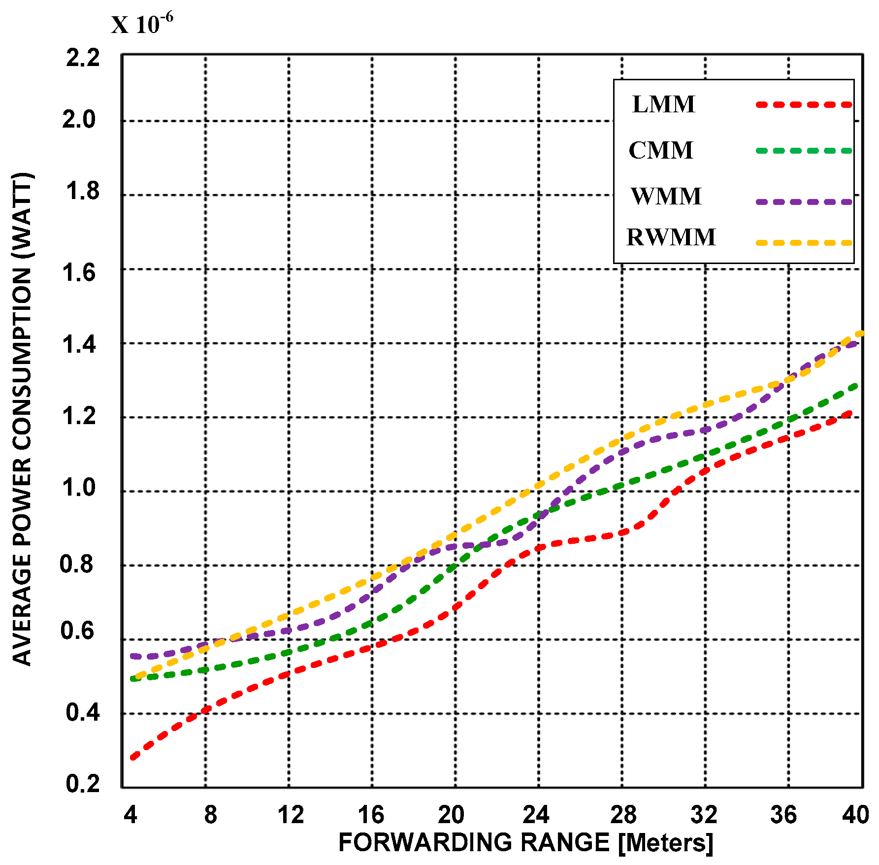
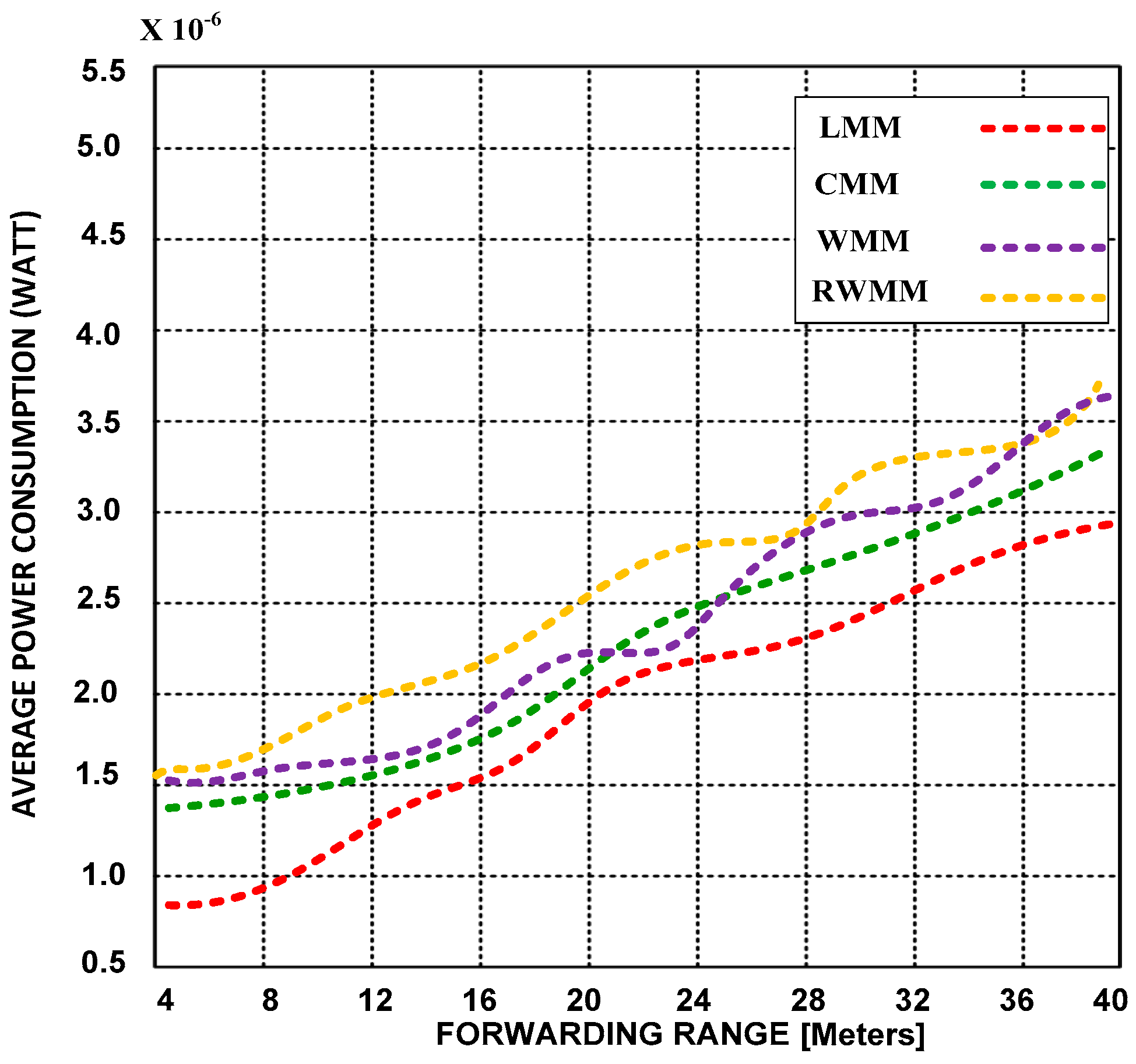
In
Figure 6 and
Figure 7, we show an average power consumption using short and long event distances and forwarding ranges.
The event area, the rate of traffic load, event ranges, forwarding ranges, number of participant nodes inside the event, traffic sources, and mobility parameters are the same as those mentioned in
Figure 4 and
Figure 5.
The simulation results demonstrate that extended forwarding range does not affect power consumption or latency. However, LMM consumes less power in short and extended forwarding ranges than CMM, RWMM and WMM. The RWMM also consumes more power than the other participants’ mobility models. We also validated based on simulation results that RWMM is not best choice for WSNs from a latency and power consumption point of view.
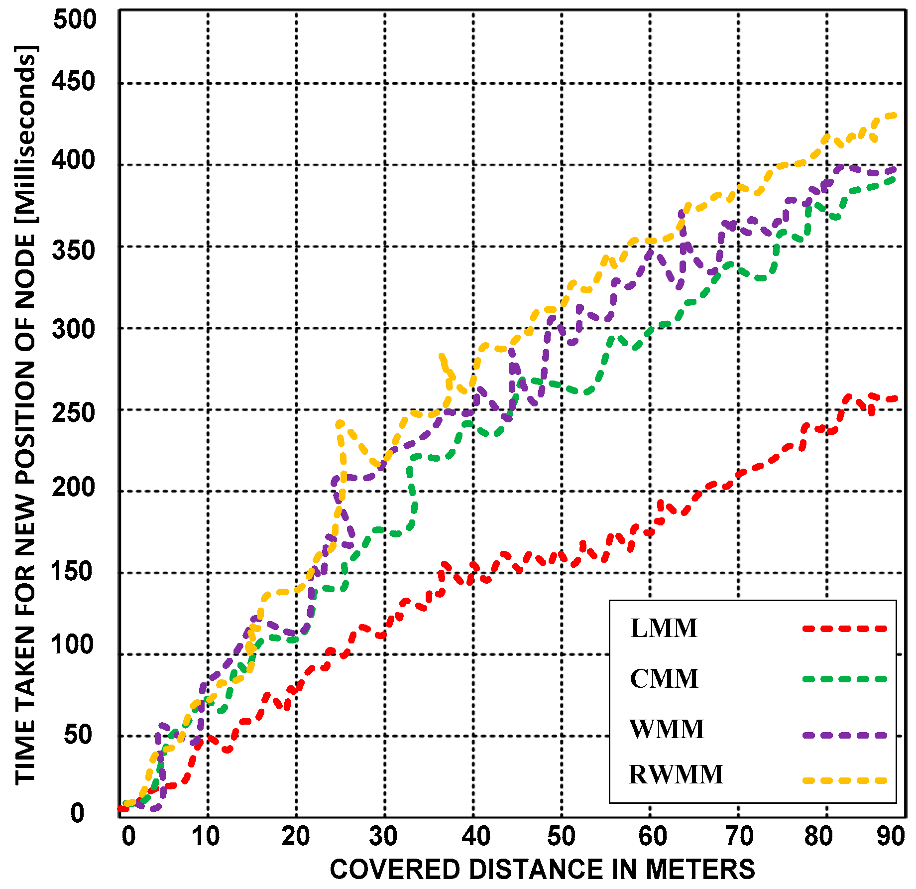
(B) Time taken by sensor nodes to reach different locations
Here, we examine the compatibility of the LMM with sensor nodes. Based on the simulation results, we analyze the time taken for each moving node to reach different positions. We also compare the efficiency of the LMM with the CMM, WMM, and RWMM.
Figure 8 presents the distances covered by the sensor nodes using the LMM and the other mobility models.
The LMM is more compatible with sensor nodes because it takes less time to change location than the other mobility models. Before letting the sensor nodes move to other locations, the LMM collects several pieces of information, including the moving location, the distance from the original location to the current location, and the distance from the current location to the destination.
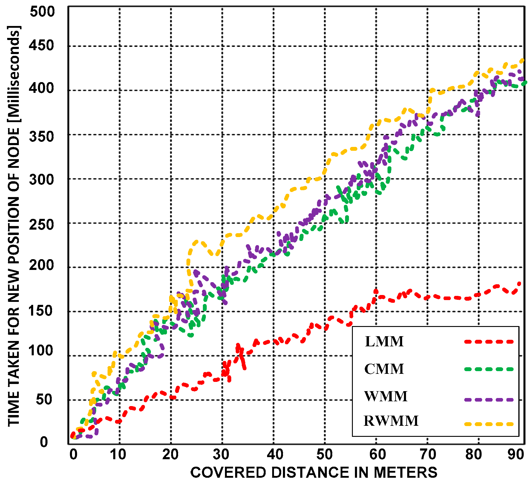
Figure 9 presents the moving times of the sensor nodes using the LMM and the other mobility models at different velocities. The LMM outperforms the other mobility models; it is scalable because the locations and the distance between the moving sensor nodes are easily determined, and the motion only marginally increases the time required to change positions.
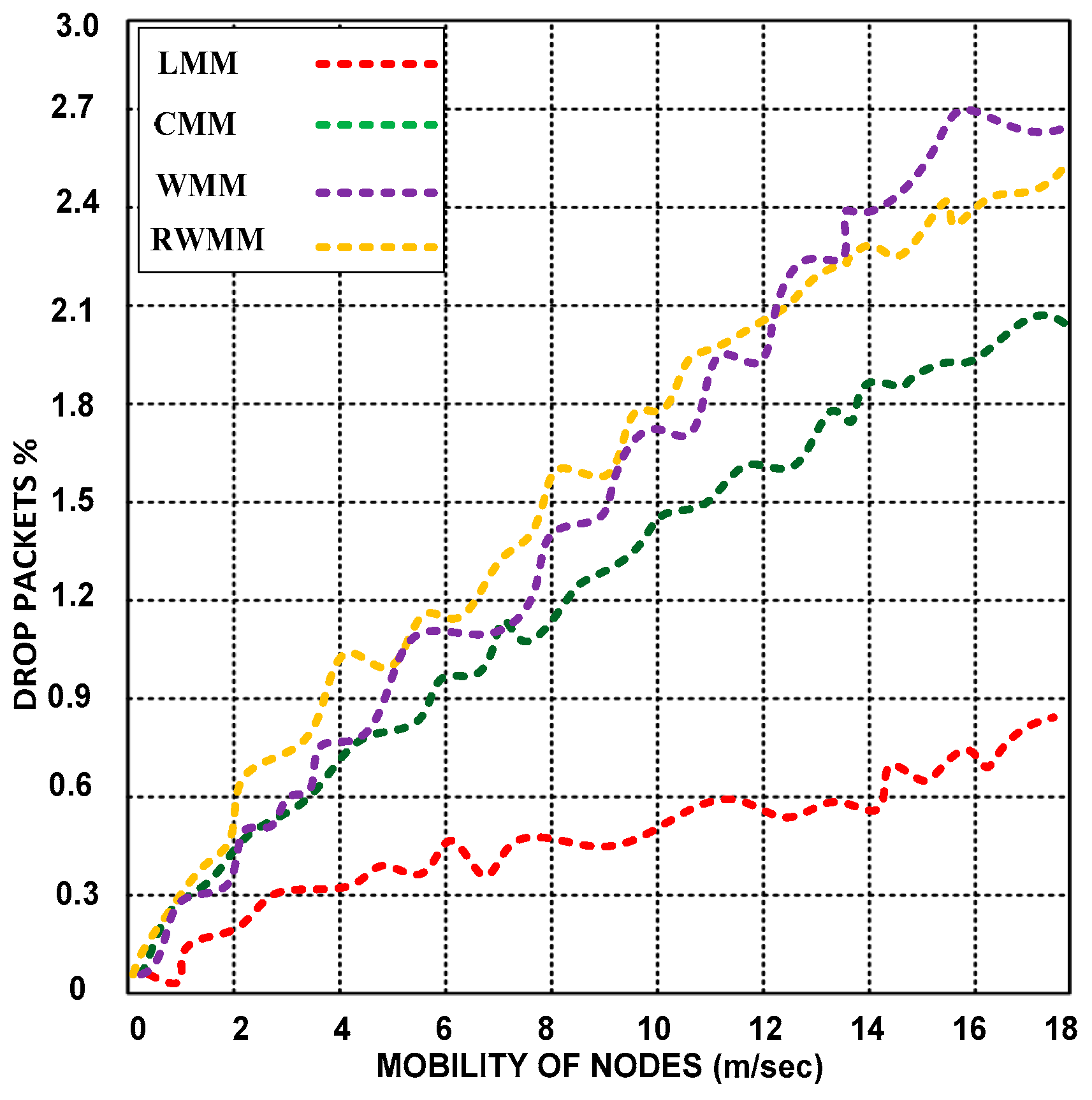
(C) Drop Rate using the LMM, CMM, RWMM, and WMM
Network congestion and a lack of network coverage are key factors that affect the drop rate of packets. These two issues are directly or indirectly dependent on the performance of the mobility models. Congestion and lack of coverage prevent packets from successfully arriving at the base station. The coverage problem includes monitoring a set of goals in the intended area. The sensor nodes collect the information from events within their communication range, and forward it to the base station. The base station may not be able to receive transmitted packets due to such coverage problems.
Figure 10 compares the packet drop rate of the LMM with those of the CMM, RWMM, and WMM. The LMM outperforms the other mobility models in walking patterns; it drops a maximum of 0.7% of the packets, whereas the other mobility models have dropped rates as high as 2.45%. This result confirms the high potential of the LMM as a mobility model for walking patterns.
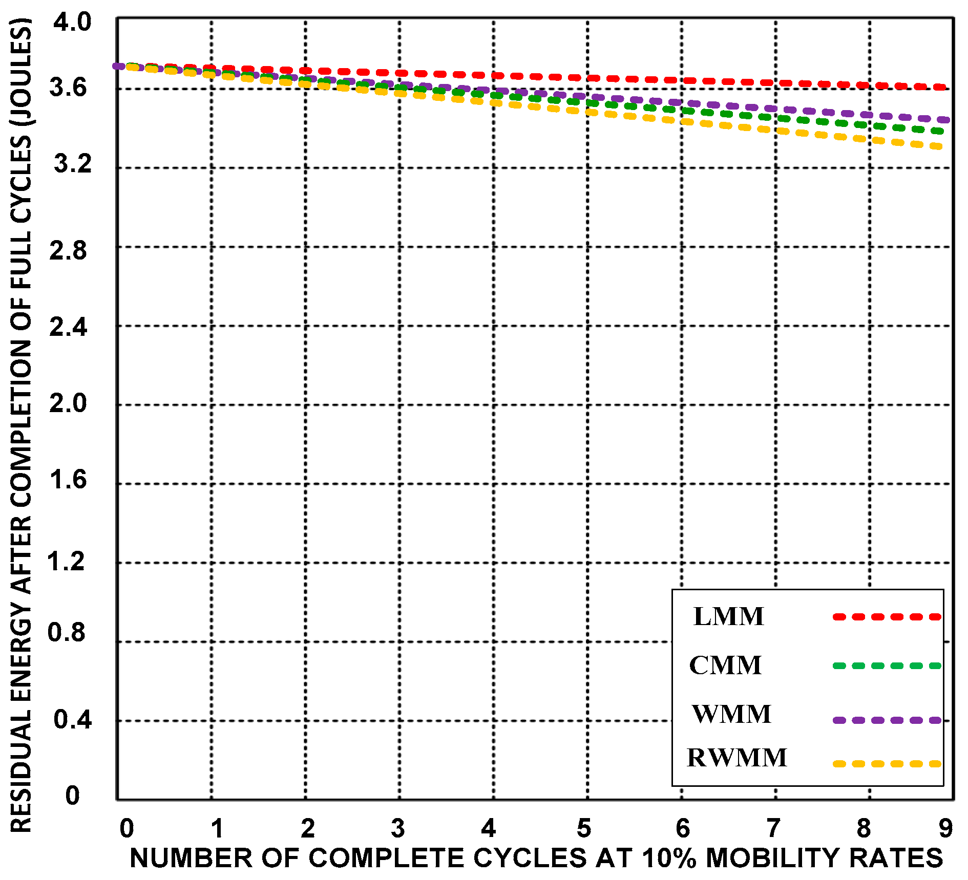
(D) Residual energy
Residual energy is the remaining energy level of the sensor nodes after completing the task. Here, we discuss the average residual energy level of the sensor nodes after changing locations.
Figure 11,
Figure 12 and
Figure 13 compare the residual energy of LMM with those of the CMM, RWMM, and WMM at 10%, 25% and 50% mobile sensor nodes. The sensor nodes have a higher residual energy with the LMM after changing location seven times.
The residual energy of the LMM decreases from 0.12 to 0.38 Joules at 10%, 25% and 50% mobility rates, which is a smaller decrease equivalent to 10.27% after completion of nine cycles than for the other mobility models. The energy levels of the other mobility models decrease from 0.28 to 0.756 Joules after completing ten motion cycles (the completion of event monitoring), which is equivalent to 20.27%. It is almost a double energy consumption waste.
(E) Time Complexity
The better performance of mobility model depends on the minimum time complexity. The time complexity is measured by manipulating the number of basic operations performed by the mobility model and constant amount of time to accomplish. Our proposed LMM gives lower time complexity as compared to other mobility models. LMM and competing mobility models are based on recursive approach. Therefore, time complexity of mobility models can be obtained using recursive approach shown in
Table 3.


