1. Introduction
Recently, the rapid dissemination of smartphones with sensing capabilities has enabled the advancement of the Human Activity Recognition (HAR) area. This advancement has benefited applications such as health care [
1,
2], monitoring physical activities [
3,
4], domestic activities [
5], and safety [
6,
7]. As a result, many solutions have been proposed based on machine learning algorithms, especially the shallow algorithms (e.g., SVM, Decision Tree, Naive Bayes and KNN) [
4,
8,
9] and, more recently, the deep learning algorithms based on neural networks (e.g., CNN, RNN, RBM, SAE, DFN and DBM) [
10,
11,
12]. The main difference between the two approaches lies in the way the data is prepared. Shallow algorithms, for example, rely on human knowledge about the problem domain to manually configure the data segmentation and reduction of data noise steps, and especially the feature extraction and feature selection steps. On the other hand, deep algorithms are able to segment data, reduce noise, and extract relevant features automatically [
10]. This has increased the efficiency of classification models and reduced human influence on HAR solutions.
Considering the limited hardware capacity of smartphones, the main problem of both approaches is still the high consumption of computational resources related to memory and processing, especially when it comes to deep neural networks. In addition, smartphones still have limited power resources, and high-cost solutions tend to drain the battery faster. Deep neural networks, for example, require a large processing capacity during the training of classification models. For this reason, the Graphic Processing Units (GPUs) [
12] available on desktop computers are used. Thus, deep learning algorithms become impractical for the development of online applications that run completely on smartphones and are not dependent on external processing (e.g., servers) [
13]. For this reason, this work focuses only on the evaluation of strategies based on shallow algorithms with the objective of proposing low-cost online solutions capable of running completely on the smartphone.
In the context of shallow algorithms, the computational cost of the solutions is concentrated in the feature extraction step. The feature extraction step is crucial for generating accurate classification models. This step consists of transforming raw sensor data into useful and compact information in order to facilitate the learning process of machine learning algorithms. For example, in the case of deep neural networks, the features are represented by the neurons of the hidden layers. In the case of shallow algorithms, the features are divided into domains of representation such as time and frequency [
14]. Time domain features are extracted by means of mathematical functions used to extract statistical information from the data. Frequency domain features are extracted by mathematical functions that capture repetitive patterns of data. In an attempt to reduce computational cost in the feature extraction step, Khan et al. [
15] proposed the use of only the time domain features. However, the use of many features generates databases with high dimensionality, influencing the processing cost of the classification model’ training step. In addition, the use of low cost classification algorithms (e.g., Naive Bayes and Decision Tree), elimination of the steps of data noise reduction, and feature selection also reduce the cost of solutions [
13].
In addition to the time and frequency domain features, the HAR literature also cites the existence Discrete domain features are extracted by means of symbolic representation algorithms like Symbolic Aggregate Approximation (SAX) [
16] and Symbolic Fourier Approximation (SFA) [
17]. These algorithms have discretization functions that transform data segments into symbols. The frequency of the symbols can evidence repetitive patterns in the data. The advantages of discrete domain features include the ability to reduce the data dimensionality and data numerosity during the feature extraction step. In the other domains, the data dimensionality reduction occurs only after the feature extraction step with the application of methods such as information gain [
18] and PCA [
15]. The fact is that the discrete domain reduces the data dimensionality in a natural way, since the symbols are compact representations of the data segments. In addition, the feature extraction process in the discrete domain is considered a natural reducer of data noise in time series [
16,
17]. From the perspective of the other domains features it is necessary to use extra methods such as Lowpass [
19] and moving average [
20] filters. In practice, the use of the discrete domain features implies a reduction in the execution of unnecessary steps of the standard HAR methodology.
In short, symbolic representation algorithms allow a massive amount of data to be reduced to a reasonable and representative number of symbols [
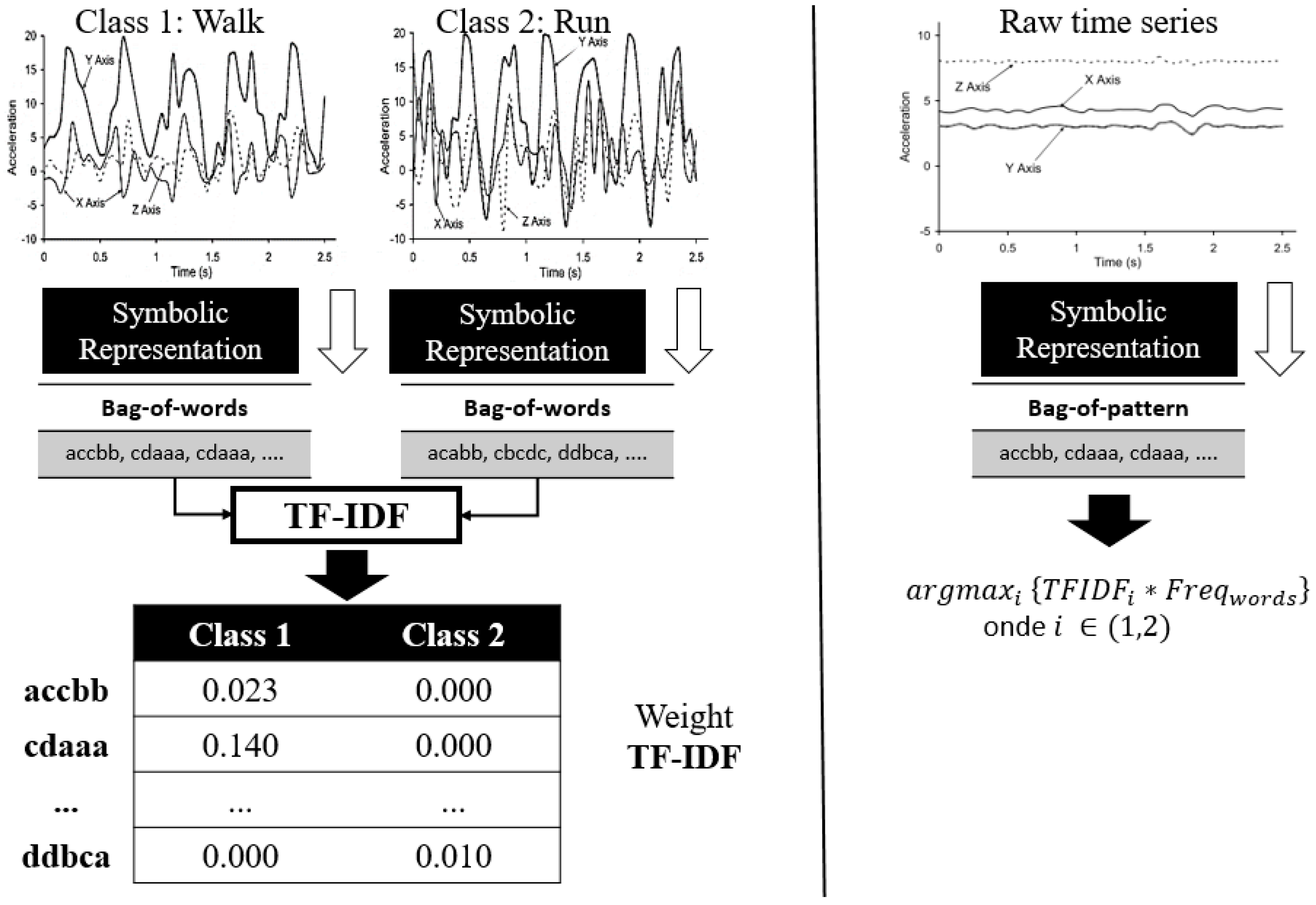
21]. This contributes to reducing the complexity and computational cost of HAR solutions, opening doors for the use of new HAR strategies in the context of smartphones with limited memory and processing resources. In relation to the learning of symbolic data, there are specific classification algorithms that can be used in the classification models training step. Some of them are extensions adapted to the SAX and SFA algorithms such as the SAX-Vector Space Model (SAX-VSM) [
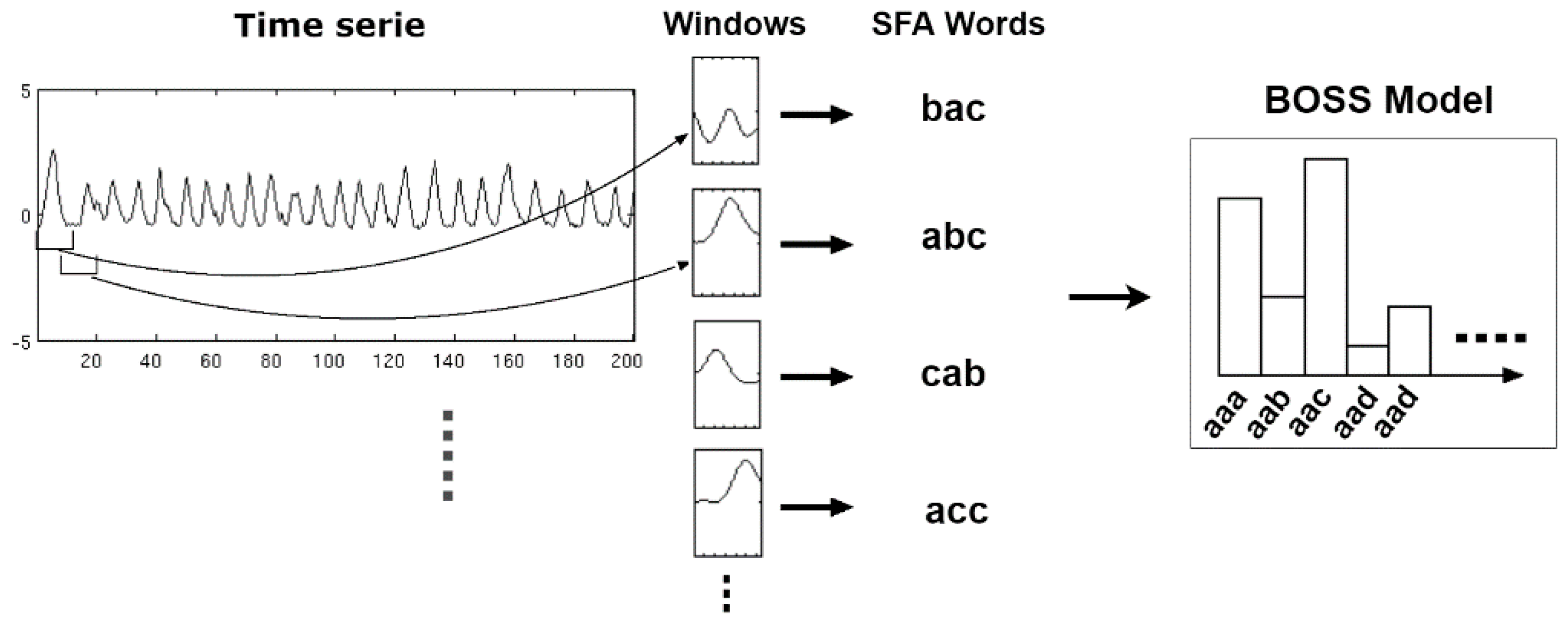
22], Bag-of-SFA Symbols (BOSS) [
23], BOSS-Vector Space (BOSS-VS) [
24], and Word Extraction for Time Series Classification (WEASEL) algorithms [
25]. However, these algorithms cannot handle time series with multiple coordinates. For this, it is necessary that all of them be adapted so that they can handle the three-dimensional inertial sensors data.
In this context, this article has two main contributions. The first one is the evaluation of SAX and SFA strategies and their extensions SAX-VSM, BOSS-VS, BOSS and WEASEL with the purpose of introducing the techniques of symbolic representation in the HAR area. The second is to propose an adaptation to the SAX-VSM, BOSS-VS, BOSS-Model and WEASEL algorithms so that they become able to handle multiple time series. The objective of this article is to improve HAR solutions based on smartphones instrumented with inertial sensors with the use of scalable and low cost strategies. The experiments were performed on three databases UCI-HAR [
26], WISDM [
27] and SHOAIB [
28]. These databases are commonly used in the literature to validate HAR solutions. The results show that the symbolic representation algorithms are more accurate than the shallow algorithms, that they are on average 84.81% faster in the feature extraction step, and that they reduce on average 94.48% of the memory space consumption.
This paper is organized as follows:
Section 2 presents the concepts related to the symbolic representation of the data.
Section 3 discusses the discretization algorithms and the process of feature extraction of the discrete domain.
Section 4 presents the classification algorithms adapted to manipulate discrete domain features.
Section 5 presents the proposals for adapting the symbolic classification algorithms to work with the multidimensional time series.
Section 6 presents the evaluation of classification models based on symbolic representation algorithms.
Section 7 presents the work related to this research. Finally,
Section 8 presents the conclusions of this work.
2. Features Representation in the Discrete Domain
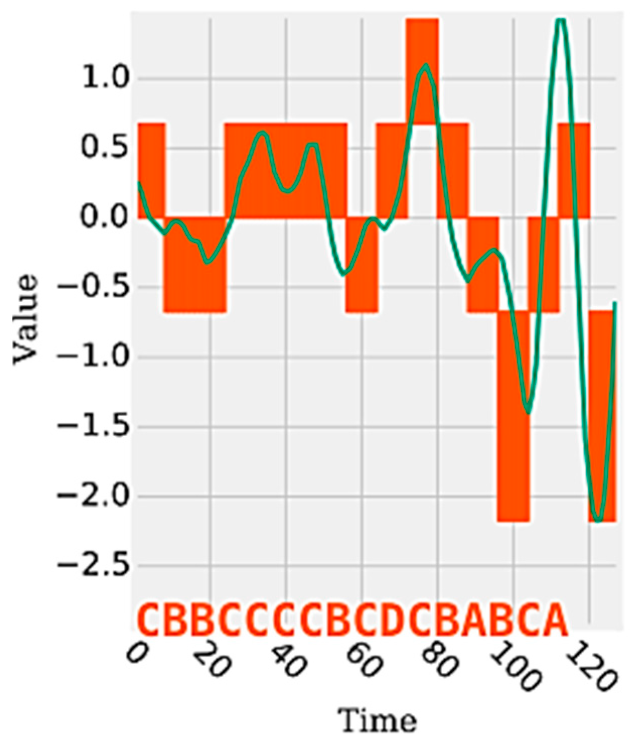
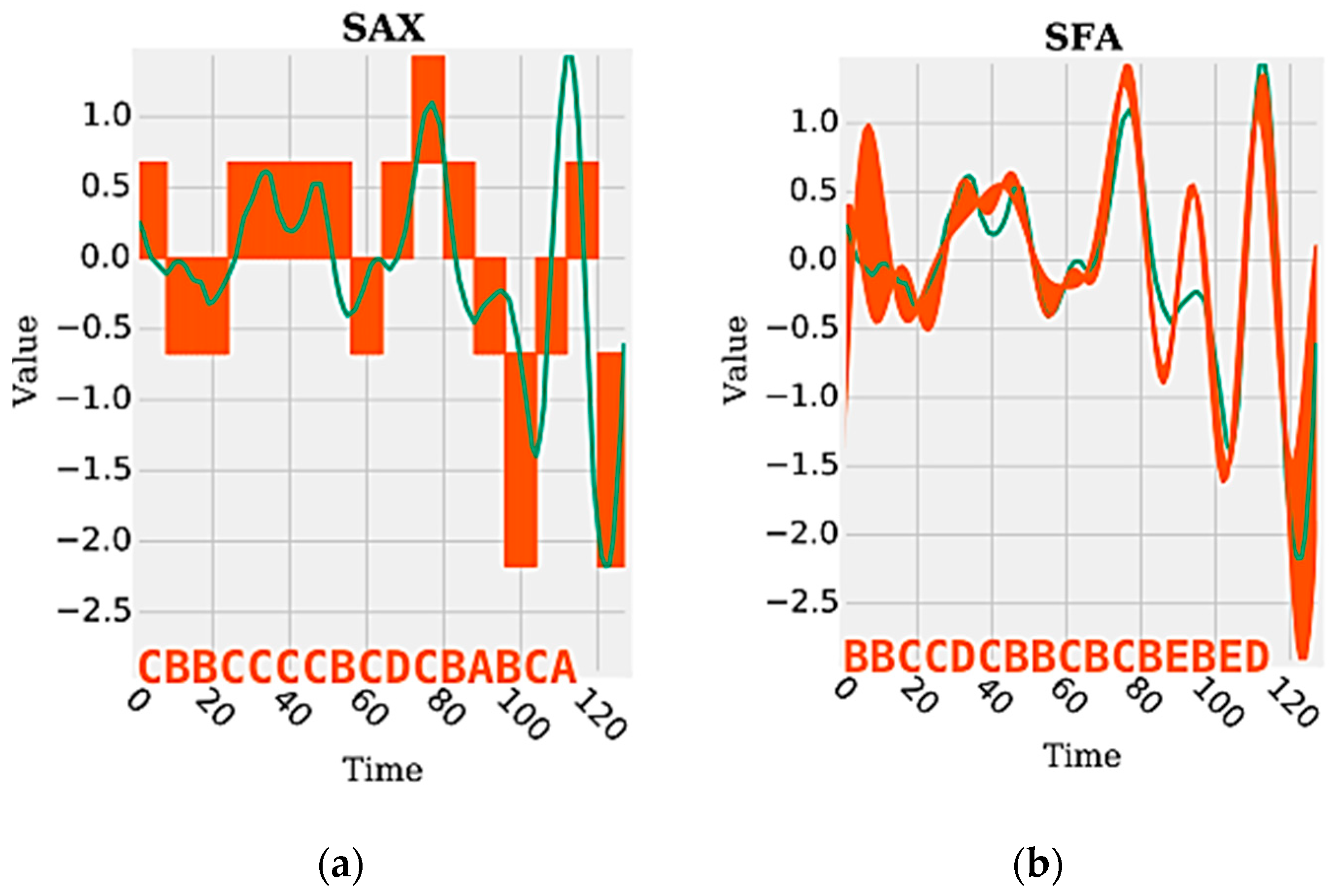
The features of the time domain and frequency domain are represented by continuous values extracted by statistical and mathematical functions applied on a set of segments of a time series. Such functions can be used to generate numerous attributes (e.g., mean, standard deviation, and variance) from the data signals generated by the sensors, which together are able to represent and discriminate a human activity. On the other hand, the data representation in the discrete domain has, as a feature, a single attribute represented by a sequence of symbolic values. Each symbol represents a range of continuous values contained in a given segment of the signal.
Figure 1 shows an example of a time series segment composed of 140 samples and represented by the word (or symbol) “cbbccccbcdcbabca”. Each word is formed by a set of letters limited by an alphabet. A word represents a numerical approximation of a subsequence composed of continuous values. Therefore, the discrete domain features are represented by a set of words, related to each other, capable of discriminating a human activity from the signals extracted from the inertial sensors.
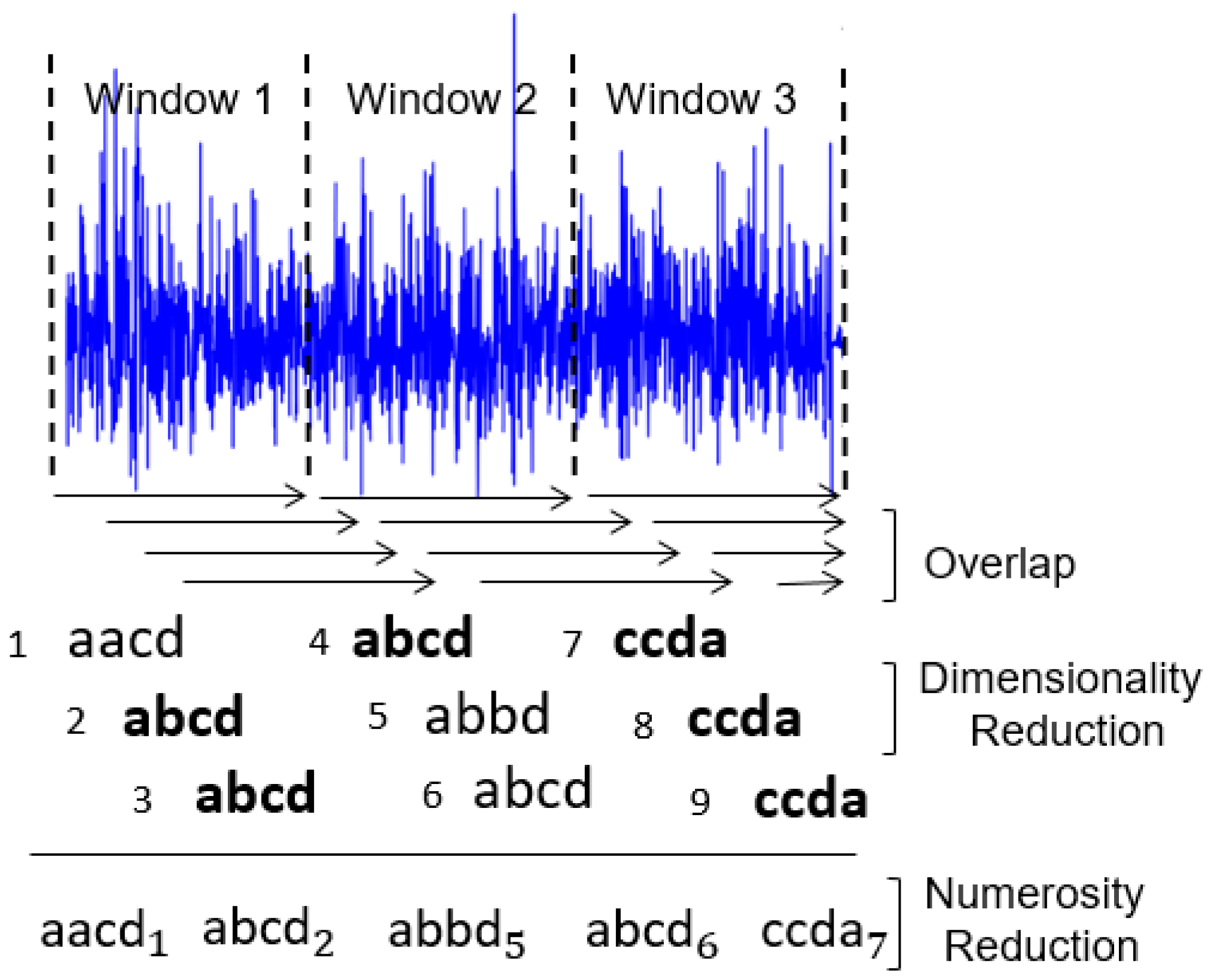
During the time series discretization, the words are organized sequentially. For each of them are assigned indexes that represent the original time series positions in which each word belongs. This sequential organization of indexed words allows reducing the amount of data after the discretization process. If there are repeated words organized sequentially, the data can be reduced further through the numerosity reduction technique. This technique adds another competitive advantage to the discrete domain features, increasing the advantage of data dimensionality reduction. Numerosity reduction is possible because the indexes represent each word positions in the original time series. In other words, given a subsequence of repeated words, only the first word must be retained and the remaining words can be deleted [
30].
Figure 2 shows an example of how dimensionality and numerosity reduction occurs in a discretized time series.
Although there are risks of information loss in the discretization process, there is a mathematical proof, demonstrated by Lin et al. [
31] and Schäfer and Högqvist [
17], which ensures that the distances between two discrete time series are equivalent to the distances of the same time series in their original state. This mathematical proof refers to the calculation of the lower bounding between raw time series and discretized time series. In addition, the calculation of the distance between two subsequences is considerably faster in the discretized series. On the other hand, there is no loss of information in the numerosity reduction process since the sequence of the omitted symbols can be easily retrieved by correctly manipulating the symbol position indexes.
5. Multidimensional Time Series
Classification algorithms mentioned above are prepared to handle only a single time series. The problem is that the data extracted from the inertial sensors have multiple time series, that is, the time series referring to the three-dimensional coordinates . For this reason, it is necessary to adopt strategies capable of adapting these algorithms to act with multiple time series or multiple variables. In this sense, this work proposes two strategies.
The first strategy consists of a change in the database format so that the symbolic classification algorithms (SAX-VSM, BOSS, BOSS vs. and WEASEL) are able to stack histograms of each coordinate synchronously. The intuition of this strategy is that several segments of different synchronized time series are organized in the same tuple with the purpose of producing the stacking effect. The advantage of this approach is that there is no need to make any changes to the Bag of Patterns strategies used by the BOSS or the Bag of Words strategy used by SAX-VSM. For this reason, any of the algorithms described in this chapter can be used. The data entry format consists of the following matrix organization of the
,
and
coordinates:
where
represents the time series for each coordinate,
represents the position of the time series values,
represents window size and
represents the position of the column. In summary, the matrix means that
,
and
are split into same-size segments, using windowing for each coordinate axis. After, the segments are concatenated with one another and the stacking works by virtue of the algorithms using the same window size
, such that words will be computed independently for
,
and
. Thus, this strategy avoids extra processing related to isolated discretization of each time series so that words are later stacked in a single histogram.
The second strategy consists of the use of data fusion techniques such as magnitude and PCA (Principal Component Analysis) for transforming the multidimensional time series into a one-dimensional time series to use the existing symbolic representation algorithms in their natural form. In the case of magnitude, the formula used to transform the coordinates is based on Equation (8):
where,
,
and
are the coordinates of the inertial sensors and
is the data sequence. In the case of PCA, only the first component is considered since it contains the main information of the components generated.
In addition, Schäfer and Leser [
37] proposed an algorithm based on the stacking of words called Weasel + MUSE. This algorithm presents a differential with the application of the derivation technique [
38] of histograms. This technique consists of relating the histograms of each coordinate by calculating the difference between the neighboring histograms of each dimension. Weasel + MUSE uses the Weasel framework, i.e., all the advantages and disadvantages of using bigrams, window size, and feature selection are incorporated into Weasel + MUSE.
6. Experiments and Results
This section presents the experimental protocol and the results concerning the comparative analyzes between the shallow algorithms and the symbolic representation algorithms. The experimental protocol presents a description of the databases used in the experiments. After, it describes the baselines with emphasis on the presentation of the time and frequency domain features. Then, the configurations and parameters used in the algorithms are presented. Finally, the results address a comparative analysis involving the study of the solutions in terms of precision, processing time, and memory consumption.
6.1. Databases Used in Experiments
The UCI-HAR database [
26] was collected with data from 30 people aged 19–48 years. Each person performed 6 physical activities such as walking, sitting, standing, lying down, and going up and down stairs. The data were collected from a Samsung Galaxy S2 handset using the accelerometer and gyroscope sensors at a frequency of 50 Hz. The collection was performed with the smartphone located at the user’s waist. All steps of data collection were recorded and the data was manually labeled. UCI-HAR has 1,311,439 samples.
The Shoaib database [
28] was collected with data from 10 male users ranging in age from 25 to 30 years. Each user performed eight activities for 3 to 4 min for each activity. Such activities include walking, running, sitting, standing, jogging slowly, biking, climbing stairs and coming down stairs. Data were collected from a Samsung Galaxy S2 (i9100) mobile phone using the accelerometer, linear accelerometer, gyroscope, and magnetometer sensors at a frequency of 50 Hz. Users were equipped with five smartphones located in five body positions including right and left pocket of the pants, waist, wrist and forearm. Shoaib has 629,977 samples.
The Wireless Sensor Data Mining (WISDM) database [
27] was collected with data from 36 users. Each user performed 6 activities such as walking, sitting, standing, lying down, and going up and down stairs. Data was collected from an Android smartphone (Nexus One, HTC Hero) at a frequency of 20 Hz. The collection was carried out with the smartphone located in the front pocket of the user’s pants. WISDM has 1,098,830 samples.
6.2. Baselines
The baselines used for comparison with the symbolic representation algorithms are the shallow algorithms including the Decision Tree, Naive Bayes, KNN (k-Nearest Neighbors) and the SVN (Support Vector Machine) commonly used in the HAR literature [
39,
40,
41,
42]. It is not the purpose of this paper to provide theoretical information on how each of these algorithms work; more details on each of them can be found in [
43]. The deep algorithms were not included in the experiments because of the high processing costs and the difficulty of implementing a solution completely dependent on the smartphone.
Shallow algorithms are trained based on the time and frequency domain features listed in
Table 2. Time domain features are represented by mathematical functions capable of extracting statistical information from the signal. On the other hand, the frequency domain features present an alternative of signal analysis based on the frequency spectrum of the values of a certain time window. The mathematical functions commonly used in this context are Fast Fourier Transform (FFT) [
44] or Wavelet [
45]. Then, the frequency features listed in
Table 2 are extracted based on the FFT or Wavelet results.
In the case of the inertial sensors, the features are extracted after the data segmentation step. This step consists of segmenting the sensor signal into time windows represented by a sequence , where represents the window size and represents an arbitrary position, such as , where represents the sequence size. In addition, time windows may overlap each other, that is, two time windows may have intersections between them. The purpose of the overlap is to minimize the number of time windows that contain different label data. Ideally, all windows have consistent data, that is, only one label. Finally, the feature extraction step consists of a data transformation process performed on top of the segmented data.
The treatment of multidimensional time series using the shallow classification algorithms based on the time and frequency domain features is simpler. This process occurs in the feature extraction step by concatenating the feature vectors of each coordinate. The result is a single database with the features of all coordinates.
6.3. Algorithm Settings and Parameters
This section presents the settings and parameters used by baselines and by the symbolic representation algorithms. A common configuration to all of them is related to the classification models evaluation strategy. In this case, the strategy adopted was cross-validation 10-folds. Each fold contains random data belonging to all users. In addition, the evaluation metric used is the accuracy. To simplify the presentation of the results, the experiments were performed only with the inertial sensor accelerometer data. According to Sousa et al. [
9] this sensor is sufficient to represent the physical activities of users. In the others, the configurations used specifically for baselines are based on results of experiments carried out in the literature [
3,
9,
46], as: (1) time window size: 5 s; (2) overlap: 50%; (3) features: time domain, frequency domain derived from FFT, and Wavelet.
In the case of the symbolic representation algorithms, this work presents the results of the multidimensional time series manipulation strategies explained in
Section 6. In addition, the parameters that must be defined are: window size, word size, and alphabet size. Some parameters were defined based on suggestions from the literature of the symbolic representation algorithms [
16,
17]. The other parameters were defined based on experiments done with the data extracted from the inertial sensors. These parameters were evaluated in the UCI-HAR database and replicated to the other databases. Thus, the configurations defined were:
Window size: algorithms were evaluated with different window sizes ranging from 20 to 250 samples. For each database, the best time window size found was equal to the number of samples contained in 1 s, that is, the value equivalent to the frequency rate of the database collection.
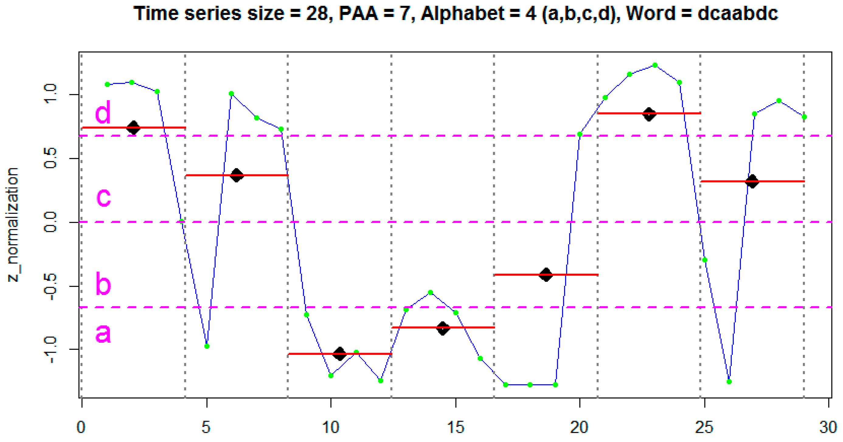
Word size: algorithms were evaluated with different word sizes ranging from 4 to 8 letters. These sizes were chosen because they are commonly used by SAX and SFA authors. In this case, it was observed that, the larger the word size, the better the accuracy of the classification models. This occurs because larger words tend to get closer to the original sequence. Therefore, the word size that was defined was 8 letters.
Alphabet size: The alphabet size was set to 4 characters, as recommended by the authors of the SAX algorithm [
16] and SFA [
17].
Experiments were run on an Intel Core i7-3612QM CPU 2.10 GHz computer equipped with 8.00 GB of RAM. The time-based experiments were run three times and averaged over time.
6.4. Results
This section presents a comparative analysis of the symbolic representation algorithms SAX-VSM, BOSS, BOSS vs. and WEASEL with the Decision Tree, Naive Bayes, KNN and SVN shallow algorithms combined with the time and frequency domain features. Results are divided into three scenarios. The first deals with the evaluation of the classification models accuracy. The second deals with the evaluation of the processing time in the steps of feature extraction and the classification models training. Finally, the third deals with the evaluation of the space consumption (memory) for each one of these steps.
6.4.1. Evaluation of the Precision of Classification Models
This section presents the results regarding the accuracy of classification models.
Table 3 and
Table 4 present a summary of the results grouped into six categories. The first category deals with the classification models generated by shallow algorithms trained with the time domain features. The second and third categories deal with the classification models generated with frequency domain features based on FFT and Wavelet. The fourth category deals with the classification models generated by the symbolic representation algorithms using the coordinate fusion strategy based on the histograms stacking. Finally, the fifth and sixth categories deal with the generation of classification models using the coordinate fusion strategies based on magnitude and the PCA.
In the context of shallow algorithms, the results show that classifiers based on time domain features are superior in terms of accuracy compared to classifiers based on frequency domain features. In this case, the highlight should be given to the Decision Tree and KNN classifiers, since both have an average accuracy rate of 89.19% and 90.77%, respectively, considering all the databases evaluated. On the other hand, the accuracy rates of the same classifiers based on frequency domain features derived from FFT and Wavelet, decreased by an average of 22.31% when compared to the results of time domain features. In addition, among all classifiers, the worst performance is Naive Bayes with an average accuracy below 66.15% for the time domain features.
These results are not new; Sousa et al. [
9], for example, reached the same conclusion and they affirm that time domain features are sufficient to represent activities from inertial sensors’ data, especially using algorithms of the decision tree family where they have a lower processing cost compared to the KNN and SVM.
In the context of the symbolic representation algorithms, the results show that all the coordinate fusion strategies using the symbolic representation algorithms BOSS and BOSS vs. offer the best results in terms of the classification models precision. In particular, the BOSS algorithm obtained an accuracy rate of 100% for all databases evaluated. This may have been caused by overfit of the parameters setting that allowed the BOSS model to suffer overfitting. The BOSS vs. classifier obtained an average accuracy rate of 97.9% confirming the overfit of the BOSS algorithm. On the other hand, the WEASEL algorithm obtained the worst accuracy with an average rate for all databases of 50.75%. This shows that Weasel is not suitable for use in combination with coordinate fusion strategies.
As can be observed, the symbolic representation algorithms obtained the best accuracy when compared to the shallow algorithms combined with the time domain features. Therefore, this proves the efficiency of these algorithms in the context of HAR in terms of the classification models’ accuracy. The next sections show the efficiency of these algorithms in terms of processing time and memory consumption.
6.4.2. Processing Time Evaluation
This section presents the results regarding the processing time of the steps feature extraction and training of classification model in the context of shallow and symbolic representation algorithms.
Table 5 shows the processing times of the feature extraction steps of the time and frequency domains and the discrete domain using the SAX, SFA and SFA-W discretization algorithms. As can be seen, the average processing time of the time and frequency domain features for the WISDM database with 1,098,830 samples is 12,461.33 milliseconds. While the average for the discretization algorithms is 1892.66 milliseconds. This represents a reduction of 84.81% considering the discrete domain in relation to the other feature domains.
In particular, SFA is the fastest algorithm (with 418 milliseconds) because SFA is optimized to treat words as a set of bits. For example, an alphabet of size 4 is represented by only 2 bits, i.e., if the alphabet letters are ‘a’, ’b’, ‘c’ and ’d’, then the representation of each letter will be ‘a = 00’, ‘b = 10’, ’c = 11’, ‘d = 01’. In this way, the processing time gain reaches 96.28% in relation to the other features domains. On the other hand, the SAX algorithm manipulates words without any optimization, and yet the processing time is 2636 milliseconds. The processing time of the SFA-W is equivalent to SAX due to the selection process of important words with the application of ANOVA Test and information gain.
Table 6 shows the processing time of training of classification models by shallow classifiers and symbolic representation classifiers. As can be seen, the results can be divided into two categories. The first category called ‘A’ involves the results of the classifiers (Naive Bayes, KNN, SAX-VSM and BOSS), considering the time threshold below 151 milliseconds.
The second category called ‘B’ involves the results of the classifiers (Decision Tree, SVM and BOSS VS), considering the time threshold above 925 milliseconds. We consider that WEASEL does not fall into the categories ‘A’ and ‘B’ because of the longer processing time. On average, the classifiers of the category ‘A’ are 80.40% faster than the Weasel and the classifiers of the category ‘B’ are 99.62% faster than the Weasel. The reason for the Weasel to be the slowest classifier is because the histograms are composed of unigrams, bigrams, and words from different window sizes. In addition, Weasel applies the Chi-Squared statistical test and uses a logistic regression to generate the model, as described in
Section 4.2.2.
Classifiers of category ‘A’, Naive Bayes, KNN, SAX-VSM and BOSS, are the ones that act faster in the step of the classification models’ training. The average processing time for these algorithms is 70.17 milliseconds. This means that these algorithms are 52 times faster than the average processing of classifiers of category ‘B’. It is important to emphasize that although some algorithms are faster in the training of the classification models step, they are not necessarily faster in the classification step. However, what happens in practice is the classification of only 1 instance over time and, therefore, it is insignificant to evaluate the processing time in this context.
In this sense, we conclude that the BOSS is the fastest algorithm since the sum of the processing time of both steps for the WISDM database, for example, is 464 milliseconds. The second fastest algorithm is the SAX-VSM with a sum of 2675 milliseconds. In addition, it is important to note that coordinate fusion strategies based on magnitude and PCA are those that require a lower cost of data processing compared to the histogram stacking strategy. More specifically, the strategy based on signal magnitude is the one that consumes fewer computational resources.
6.4.3. Memory Consumption Evaluation
This section presents the results regarding memory consumption before and after the application of the feature extraction step for the UCI-HAR, WISDM and SHOAIB databases. The results are described in
Table 7 as the unit of measurement Bytes. The strategy used to collect this data was as follows. The first step consists of calculating the number of Bytes occupied by raw data in RAM memory. The second step consists of applying the feature extraction process. The third step is calculating the number of Bytes occupied by processed data in RAM memory. For the frequency domain only the features derived from the FFT were chosen, since the features derived from Wavelet have similar results. For the discrete domain, the SAX algorithm was chosen to discretize the database.
As can be seen, the time features can reduce the original data by 73.90%, on average, for all databases. For example, UCI-HAR data has been reduced from around 43 million bytes to about 9 million bytes. For frequency features the data reduction rose to 92.66%. The reason is that the number of frequency features is 68.96% smaller compared to the time features, i.e., the experiments were performed with 29 time features and nine frequency features as shown in
Table 2. On the other hand, the discrete features reduce, on average, the memory space by 94.48%, a growth of 1.92% in relation to the frequency features.
7. Related Work
In general, the literature presents two groups of discretization algorithms [
17]. The first group deals with the numerical approximation algorithms including Discrete Fourier Transform (DFT) [
45], Discrete Wavelet Transform (DWT) [
45], Chebyshev Polynomials (CP) [
47], Piecewise Linear Approximation (PLA) [
48], Piecewise Aggregate Approximation (PAA) [
32] and Adaptive Piecewise Constant Approximation (APCA) [
49]. The second group deals with symbolic representation algorithms including Symbolic Aggregate Approximation (SAX) [
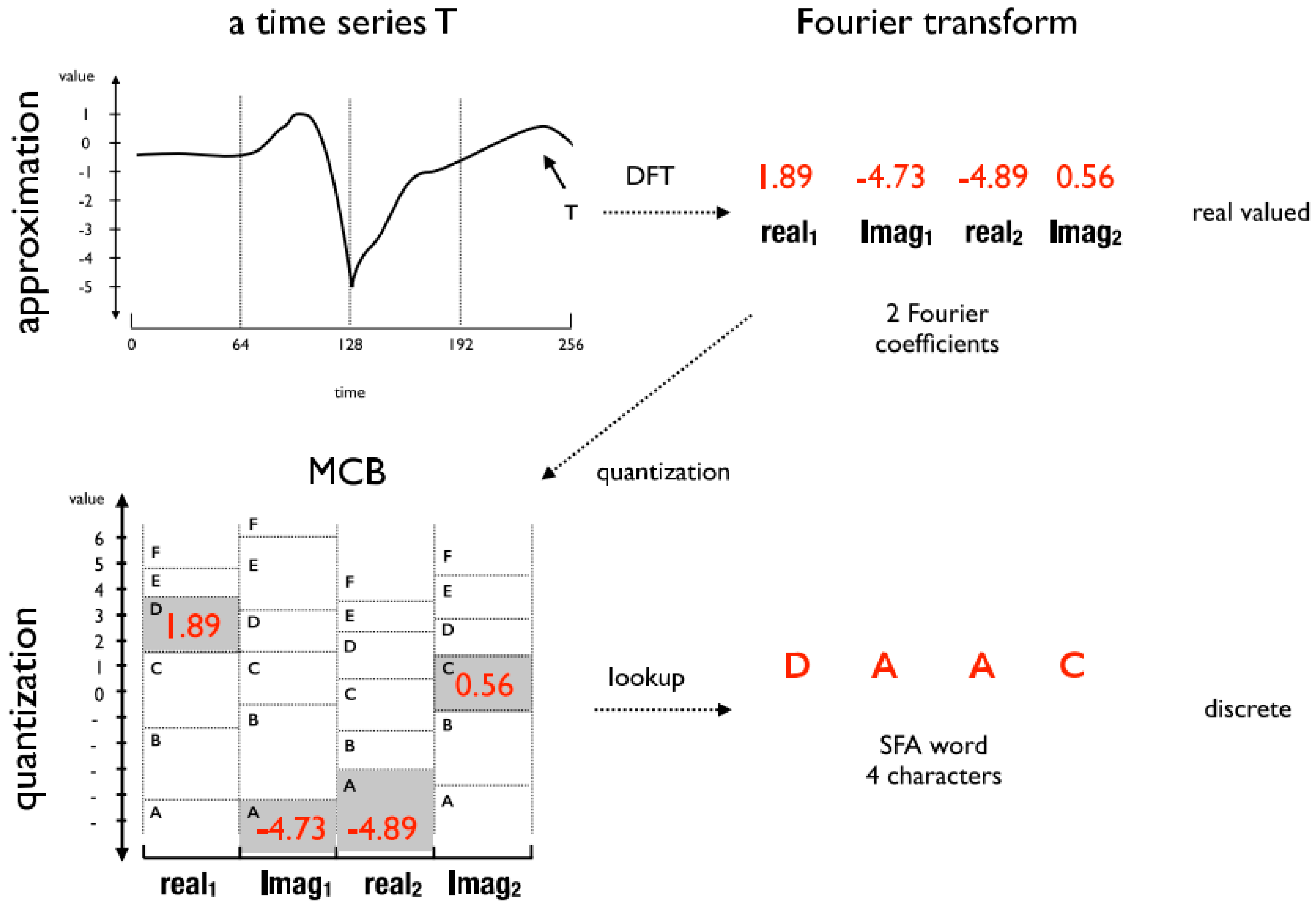
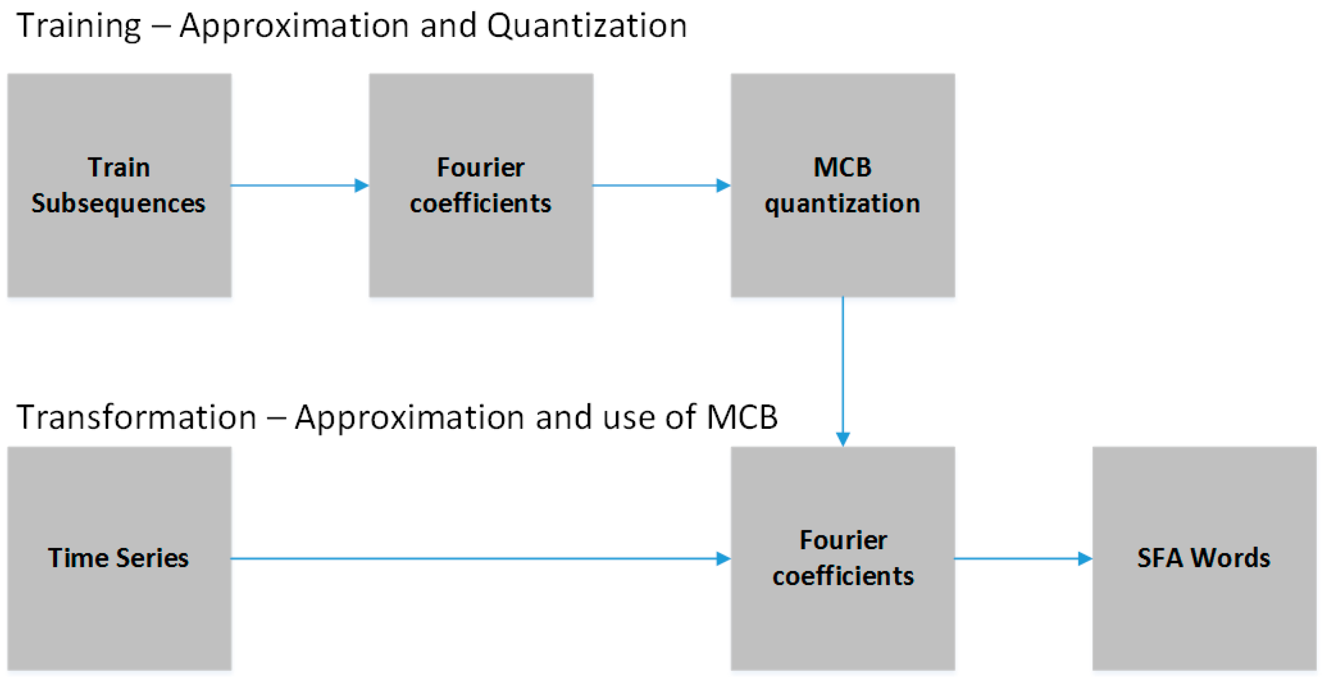
16] and Symbolic Fourier Approximation (SFA) [
17]. Specifically, this research focuses on the algorithms of the second group for two reasons. The first reason is that these algorithms are considered state of the art of symbolic representation algorithms. The second reason is that all the algorithms of the second group are based on some algorithm of the first group. For example, SAX and SFA define the symbol patterns based on the PAA and the DFT coefficients, respectively.
Symbolic representation algorithms have been used to recognize recurrent (Motifs) [
16] or anomalous (Discords) [
30,
50] patterns in time series. In the context of HAR, there are few works which use the symbolic representation algorithms [
14,
51,
52]. Figo et al. [
14], for example, use the SAX algorithm to discretize the time series. The activities classification process occurs by calculating the distance between the symbols. In this case, they used the Euclidean distances, Levenshtein [
53] and Dynamic Time Warping (DTW) [
54]. In the experiments a comparative analysis was performed between discrete features and time features (e.g., mean, variance, and standard deviation) and frequency features (e.g., entropy and energy). The data used were obtained from the accelerometer sensor and the activities evaluated were jump, run, and walk.
Siirtola et al. [
51] proposed a new method called SAXS (Symbolic Aggregate approximation Similarity). SAXS consists of defining prototypes for each activity, so that each of them is represented by a generic word called a template. The activities classification process occurs by calculating the similarity between a new non-labeled word and the templates of each activity. Thus, the new word is sorted based on the closest template, i.e., with the most similarity. In the experiments, a comparative analysis was performed between the features extracted with SAXS and some time features (mean, standard deviation, median, quartiles, minimum, and maximum) and frequency features (sum of coefficients and zero crossing). The data used were obtained and five public databases and activities evaluated were of movement (e.g., walking, running), gestures and swimming. The evaluated classifiers were the decision tree, KNN and Naive Bayes. The results show that SAXS is capable of increasing accuracy by 3% and by up to 10% if combined with the discrete features and the time and frequency features.
Terzi et al. [
52] also use SAX to extract the discrete domain features. In the classification of activities, the solution uses an adaptation of the k-NN to verify the minimum distance between labeled and non-labeled words. Finally, an extension of the SAX is proposed for manipulating multidimensional time series. In this case, what occurs is a linear combination of the minimum distances for each coordinate. The experiments were carried out in the UCI HAR database and evaluated the activities walking, and climbing and descending stairs. The results show accuracies of 99.54% and 97.07% for the respective classes of activities.
8. Conclusions
This work introduced and evaluated two algorithms for data symbolic representation, SAX and SFA, in the context of HAR based on smartphones instrumented with inertial sensors. These algorithms act in the feature extraction step and are responsible for generating features belonging to the discrete domain. The advantages of using symbolic representation algorithms include reducing dimensionality and numerosity of the data. In addition, these algorithms make two steps of traditional HAR methodology obsolete. The first step deals with the data noise reduction and the second step deals with the feature selection. In addition, this work evaluated some classification algorithms adapted to manipulate symbolic data, such as SAX-VSM, BOSS, BOSS-VS and WEASEL. In addition, this work proposed two strategies to manipulate multidimensional time.
Experiments were performed in three UCI-HAR, SHOAIB and WISDM databases and the results show the efficiency of the strategy based on symbolic representation algorithms in three perspectives: classification model accuracy, processing time of feature extraction, processing time of classification model training and memory consumption. The main conclusions drawn from these algorithms are:
- (1)
The BOSS and BOSS vs. algorithms obtained the best accuracy rates using the three coordinate fusion strategies (histogram stacking, magnitude, and PCA).
- (2)
The Weasel algorithm did not perform well with coordinate fusion strategies.
- (3)
The merging strategy based on coordinate histogram stacking has generated the best classifiers.
- (4)
Processing time in the feature extraction step is faster with discrete domain features. In average, discrete features are 84.81% faster compared to the time and frequency features. SFA is the fastest method taking an average of 418 milliseconds for a database with amount of data around 1 million samples (WIDSM).
- (5)
Extraction of discrete domain features is rapid using SFA due to the optimization process based on the data transformation for bits.
- (6)
SAX-VSM and BOSS algorithms are the fastest algorithms in the feature extraction and training classification models steps, surpassing all the baselines. On the other hand, the BOSS vs. and Weasel algorithms are the slowest algorithms in the training classification models step.
- (7)
Discrete domain features reduce memory consumption by 94.48% compared to the frequency features with 92.66% and time features with 73.90%. Although the space memory difference between frequency features and the discrete features is only 1.92%, the frequency features lose in terms of classification model accuracy and processing time.
Therefore, it is concluded that strategies based on symbolic representation algorithms are able to reduce the computational cost of HAR solutions, enabling their implementation in smartphones with limited memory and processing resources.

 ,
, 


