TD-LSTM: Temporal Dependence-Based LSTM Networks for Marine Temperature Prediction


Abstract
1. Introduction
2. Preliminary
2.1. Problem Formulation
2.2. Long Short-Term Memory
3. Methodology
3.1. Temporal Dependence Analysis
3.2. Structure of TD-LSTM Networks
3.3. Algorithm and Optimization
| Algorithm 1 Training of TD-LSTM networks |
| Input: |
| historical observations:; |
| target at time t: ; |
| lengths of closeness, period, trend: ; |
| period: p; |
| Output: |
| TD-LSTM model ; |
| //construct training instance |
| 1: ; |
| 2: for all available time interval do |
| 3: ; |
| 4: ; |
| 5: put a training instance () into ; |
| 6: end for |
| // train model |
| 7: initialize parameter ; |
| 8: repeat |
| 9: randomly select a batch of instances from ; |
| 10: find by optimization algorithm; |
| 11: until the objective is minimized |
| 12: output the optimized TD-LSTM model ; |
4. Experiment
4.1. Settings
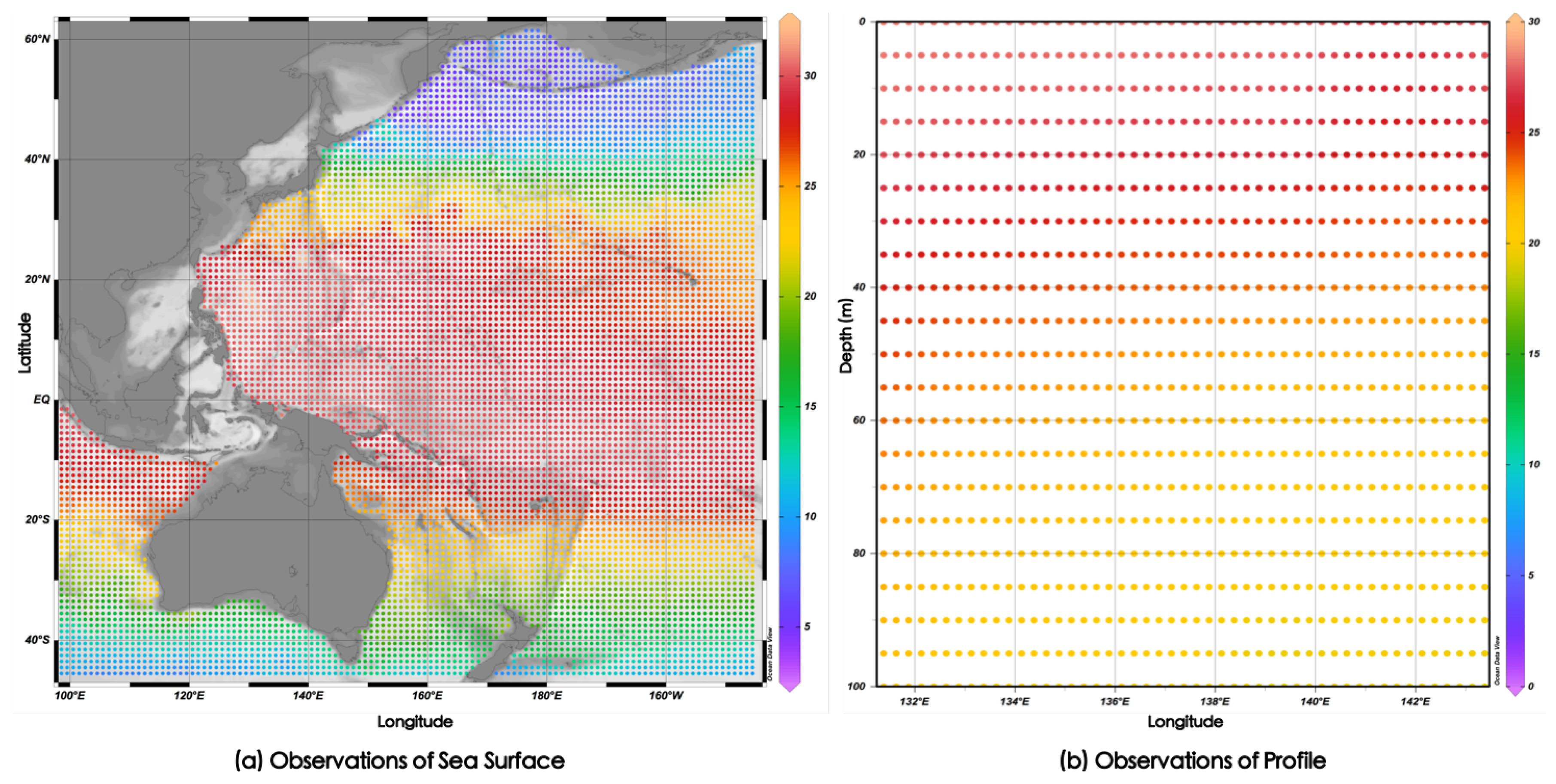
4.1.1. Datasets
4.1.2. Baselines
- SVRSupport Vector Regression (SVR) is one of the most popular regression models in recent years. SVR has achieved good results in many applications. In the experiment, we used support vector regression with the RBF kernel function.
- MLPRMultilayer Perceptron Regressor (MLPR) is a typical artificial neural network for regression tasks. We used a three-layer perceptron network, which includes one hidden layer with 100 neurons. In the MLPR network, we set and .
- LSTMLSTM is a time-recurrent neural network. Thanks to its unique design structure, LSTM can learn long-term correlation. In the experiment, we used 8 and 24 m LSTM to compare with our proposed method.
4.1.3. Preprocessing
4.1.4. Hyperparameters
4.1.5. Evaluation Metric
4.2. Evaluation of SST Prediction
4.3. Results of Different TD-LSTM Variants
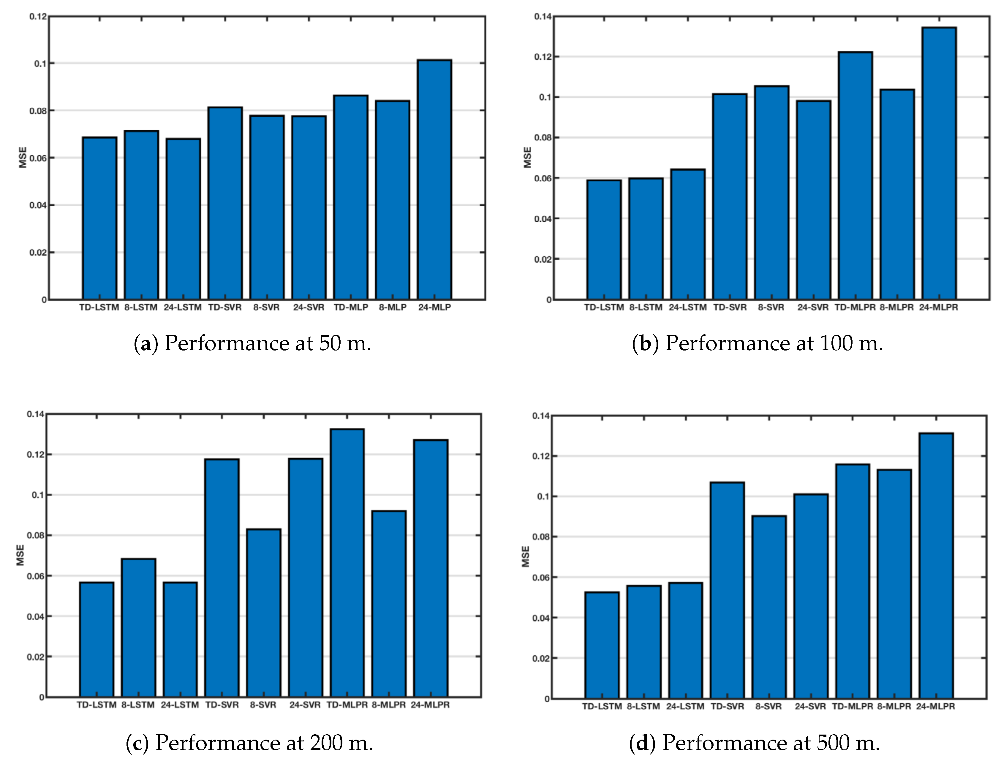
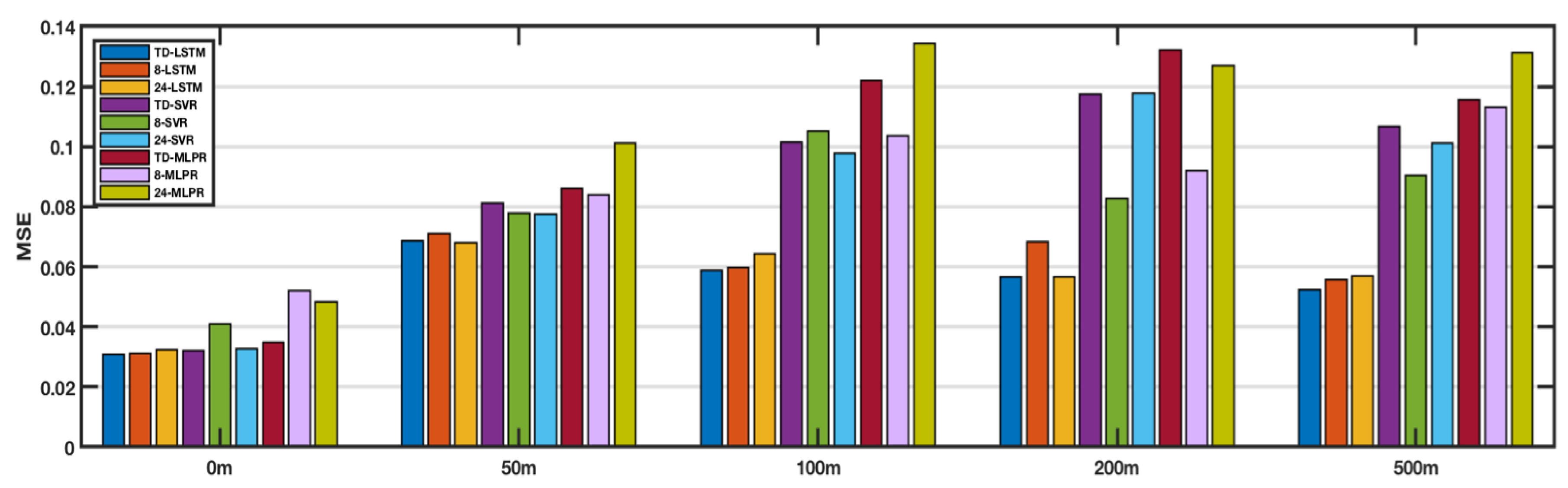
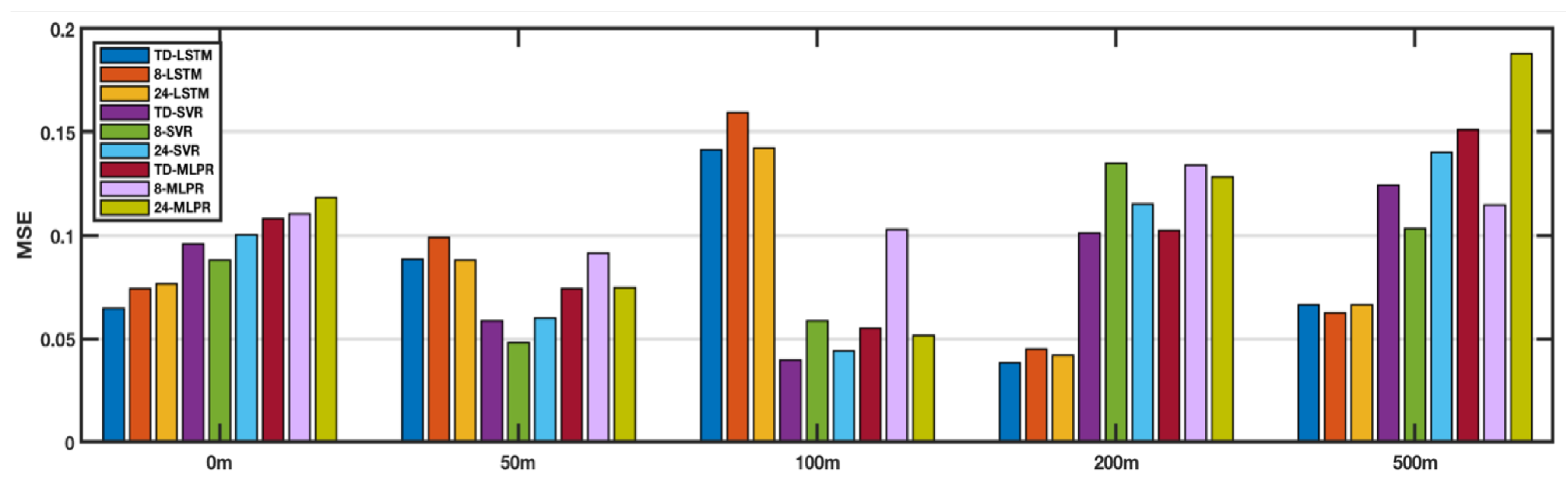
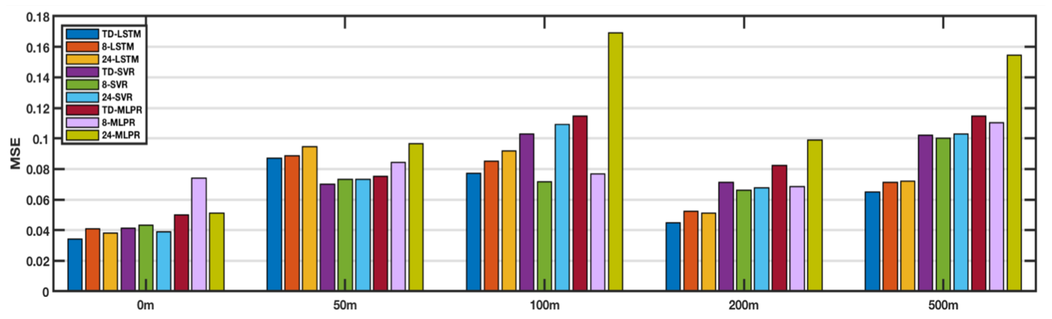
4.3.1. Comparisons of Different Ocean Depth
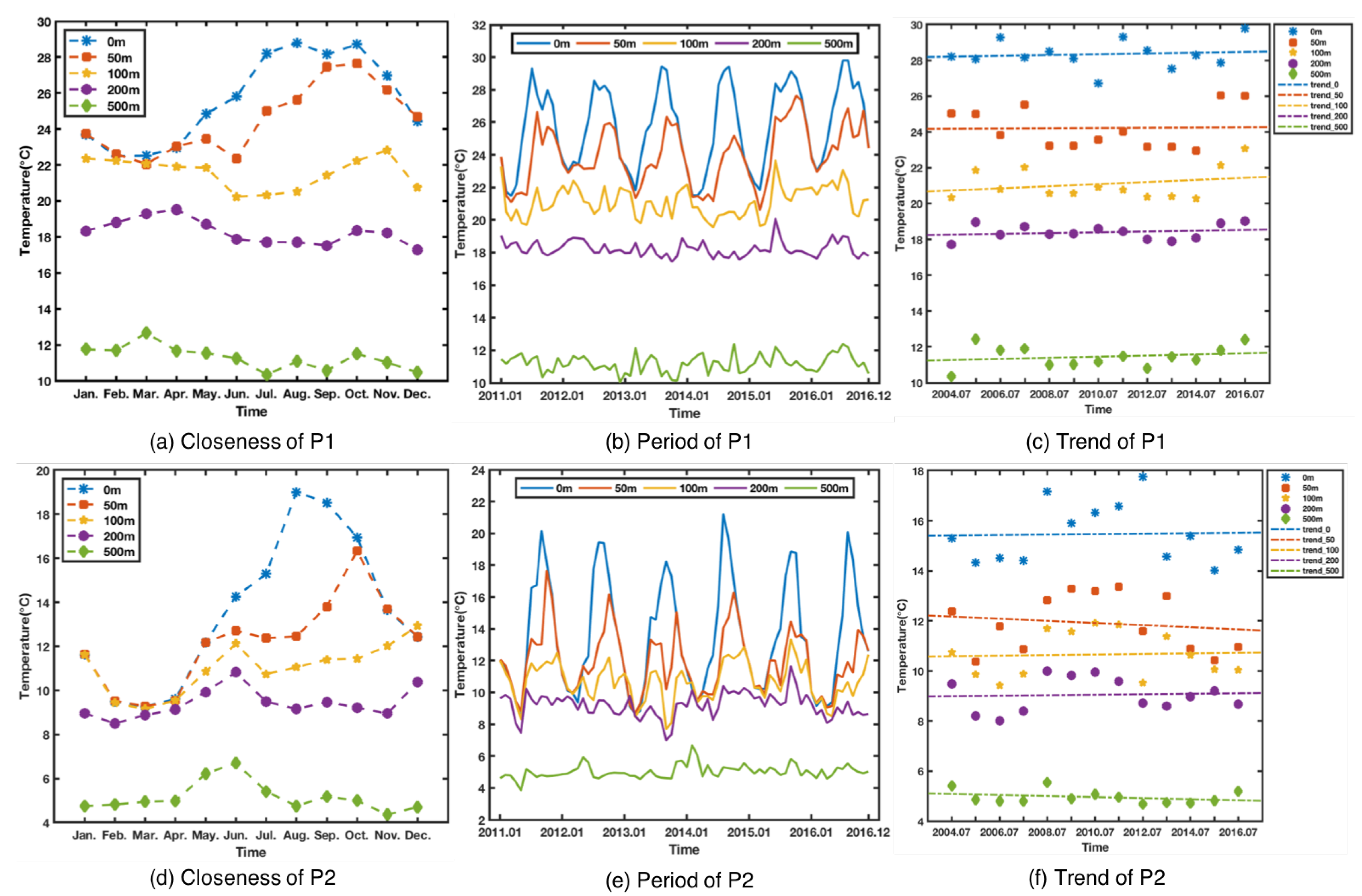
4.3.2. Impact of Temporal Closeness, Period and Trend
4.4. Comparisons of Different Regions
5. Conclusions
Author Contributions
Funding
Conflicts of Interest
References
- Millero, F.J.; Leung, W.H. The thermodynamics of seawater at one atmosphere; erratum. Am. J. Sci. 1976, 276, 1035–1077. [Google Scholar] [CrossRef]
- Han, G.; Jiang, J.; Sun, N.; Shu, L. Secure communication for underwater acoustic sensor networks. IEEE Commun. Mag. 2015, 53, 54–60. [Google Scholar] [CrossRef]
- Ingleby, B.; Huddleston, M. Quality control of ocean temperature and salinity profiles—Historical and real-time data. J. Mar. Syst. 2007, 65, 158–175. [Google Scholar] [CrossRef]
- Han, G.; Shen, S.; Song, H.; Yang, T.; Zhang, W. A Data Collection Scheme based on a Stratification Model in Underwater Acoustic Sensor Networks. IEEE Trans. Veh. Technol. 2018. [Google Scholar] [CrossRef]
- Han, G.; Jiang, J.; Bao, N.; Wan, L. Routing protocols for underwater wireless sensor networks. Commun. Mag. IEEE 2015, 53, 72–78. [Google Scholar] [CrossRef]
- Lins, I.D.; Araujo, M.; das Chagas Moura, M.; Silva, M.A.; Droguett, E.L. Prediction of sea surface temperature in the tropical Atlantic by support vector machines. Comput. Stat. Data Anal. 2013, 61, 187–198. [Google Scholar] [CrossRef]
- Arx, W.S.V. An Introduction to Physical Oceanography. Am. J. Phys. 2005, 30, 775–776. [Google Scholar] [CrossRef]
- Patil, K.; Deo, M.C.; Ravichandran, M. Prediction of Sea Surface Temperature by Combining Numerical and Neural Techniques. J. Atmos. Ocean. Technol. 2016, 33. [Google Scholar] [CrossRef]
- Xue, Y.; Leetmaa, A. Forecasts of tropical Pacific SST and sea level using a Markov model. Geophys. Res. Lett. 2000, 27, 2701–2704. [Google Scholar] [CrossRef]
- Collins, D.C.; Reason, C.J.C.; Tangang, F. Predictability of Indian Ocean sea surface temperature using canonical correlation analysis. Clim. Dyn. 2004, 22, 481–497. [Google Scholar] [CrossRef]
- Tangang, F.T.; Hsieh, W.W.; Tang, B. Forecasting the equatorial Pacific sea surface temperatures by neural network models. Clim. Dyn. 1997, 13, 135–147. [Google Scholar] [CrossRef]
- Wu, A.; Hsieh, W.W.; Tang, B. 2006 Special issue: Neural network forecasts of the tropical Pacific sea surface temperatures. Neural Netw. 2006, 19, 145. [Google Scholar] [CrossRef] [PubMed]
- Tripathi, K.C.; Rai, S.; Pandey, A.C.; Das, I.M.L. Southern Indian Ocean SST indices as early predictors of Indian Summer monsoon. Indian J. Geo-Mar. Sci. 2008, 37, 70–76. [Google Scholar]
- Lecun, Y.; Bengio, Y.; Hinton, G. Deep learning. Nature 2015, 521, 436. [Google Scholar] [CrossRef] [PubMed]
- Graves, A.; Liwicki, M.; Bunke, H.; Bunke, H. A Novel Connectionist System for Unconstrained Handwriting Recognition. IEEE Trans. Pattern Anal. Mach. Intell. 2009, 31, 855–868. [Google Scholar] [CrossRef] [PubMed]
- Zhang, Q.; Wang, H.; Dong, J.; Zhong, G.; Sun, X. Prediction of Sea Surface Temperature using Long Short-Term Memory. IEEE Geosci. Remote Sens. Lett. 2017, 14, 1745–1749. [Google Scholar] [CrossRef]
- Yang, Y.; Dong, J.; Sun, X.; Lima, E.; Mu, Q.; Wang, X. A CFCC-LSTM Model for Sea Surface Temperature Prediction. IEEE Geosci. Remote Sens. Lett. 2018, 15, 207–211. [Google Scholar] [CrossRef]
- Fustes, D.; Cantorna, D.; Dafonte, C.; Arcay, B.; Iglesias, A.; Manteiga, M. A cloud-integrated web platform for marine monitoring using GIS and remote sensing. Application to oil spill detection through SAR images. Future Gener. Comput. Syst. 2014, 34, 155–160. [Google Scholar] [CrossRef]
- Hochreiter, S.; Schmidhuber, J. Long short-term memory. Neural Comput. 1997, 9, 1735–1780. [Google Scholar] [CrossRef] [PubMed]
- Zhang, J.; Zheng, Y.; Qi, D.; Li, R.; Yi, X.; Li, T. Predicting Citywide Crowd Flows Using Deep Spatio-Temporal Residual Networks. Artif. Intell. 2018, 259, 147–166. [Google Scholar] [CrossRef]
- Hecht-Nielsen, R. Theory of the Back-Propagation Neural Network; Harcourt Brace & Co.: New York, NY, USA, 1989; Volume 1, pp. 593–605. [Google Scholar]
- Kingma, D.P.; Ba, J. Adam: A Method for Stochastic Optimization. arXiv 2014, arXiv:1412.6980. [Google Scholar]
- Liu, Z.; Wu, X.; Xu, J.; Li, H.; Lu, S.; Sun, C.; Cao, M. Fifteen Years of Ocean Observations with China Argo. Adv. Earth Sci. 2016, 6, 145–153. [Google Scholar] [CrossRef]
- Goodfellow, I.; Bengio, Y.; Courville, A.; Bengio, Y. Deep Learning; MIT Press Cambridge: Cambridge, MA, USA, 2016; Volume 1. [Google Scholar]


| Methods | P1 | P2 | P3 | P4 | P5 | Average of MSE |
|---|---|---|---|---|---|---|
| TD-LSTM | 0.0525 | 0.0319 | 0.0158 | 0.0305 | 0.0232 | 0.0308 |
| 8-LSTM | 0.0576 | 0.0293 | 0.0129 | 0.0287 | 0.0280 | 0.0313 |
| 24-LSTM | 0.0611 | 0.0314 | 0.0162 | 0.0297 | 0.0227 | 0.0322 |
| TD-SVR | 0.0368 | 0.0269 | 0.0296 | 0.0321 | 0.0348 | 0.0321 |
| 8-SVR | 0.0414 | 0.0500 | 0.0203 | 0.0536 | 0.0403 | 0.0411 |
| 24-SVR | 0.0389 | 0.0229 | 0.0294 | 0.0455 | 0.0267 | 0.0327 |
| TD-MLPR | 0.0361 | 0.0316 | 0.0353 | 0.0428 | 0.0288 | 0.0349 |
| 8-MLPR | 0.0622 | 0.0580 | 0.0302 | 0.0689 | 0.0411 | 0.0521 |
| 24-MLPR | 0.0617 | 0.0282 | 0.0503 | 0.0715 | 0.0295 | 0.0482 |
| Region | Coral Sea | Equatorial Pacific Region | South China Sea | ||||||
|---|---|---|---|---|---|---|---|---|---|
| Methods | 0 m | 200 m | 500 m | 0 m | 200 m | 500 m | 0 m | 200 m | 500 m |
| 8-LSTM | 1.7% | 17% | 5.7% | 13.2% | 14.2% | −6.0% | 16.0% | 13.9% | 8.8% |
| 24-LSTM | 4.6% | −0.4% | 7.9% | 15.5% | 8.3% | 0.03% | 10.3% | 11.9% | 10.1% |
| TD-SVR | 4% | 51.7% | 50.8% | 32.4% | 62.1% | 46.5% | 7.2% | 36.8% | 36.4% |
| 8-SVR | 25.2% | 31.5% | 41.9% | 26.4% | 71.6% | 35.8% | 20.3% | 31.8% | 35.2% |
| 24-SVR | 5.9% | 51.8% | 48.1% | 35.4% | 66.7% | 52.6% | 3.9% | 33.7% | 37.1% |
| TD-MLPR | 11.9% | 57.1% | 54.6% | 40.3% | 62.5% | 56.1% | 31.4% | 45.4% | 43.4% |
| 8-MLPR | 40.9% | 38.3% | 53.6% | 41.4% | 71.3% | 42.1% | 53.7% | 34.5% | 41.2% |
| 24-MLPR | 36.2% | 55.4% | 60% | 45.2% | 70.0% | 64.6% | 32.9% | 54.5% | 58.0% |
© 2018 by the authors. Licensee MDPI, Basel, Switzerland. This article is an open access article distributed under the terms and conditions of the Creative Commons Attribution (CC BY) license (http://creativecommons.org/licenses/by/4.0/).
Share and Cite
Liu, J.; Zhang, T.; Han, G.; Gou, Y. TD-LSTM: Temporal Dependence-Based LSTM Networks for Marine Temperature Prediction. Sensors 2018, 18, 3797. https://doi.org/10.3390/s18113797
Liu J, Zhang T, Han G, Gou Y. TD-LSTM: Temporal Dependence-Based LSTM Networks for Marine Temperature Prediction. Sensors. 2018; 18(11):3797. https://doi.org/10.3390/s18113797
Chicago/Turabian StyleLiu, Jun, Tong Zhang, Guangjie Han, and Yu Gou. 2018. "TD-LSTM: Temporal Dependence-Based LSTM Networks for Marine Temperature Prediction" Sensors 18, no. 11: 3797. https://doi.org/10.3390/s18113797
APA StyleLiu, J., Zhang, T., Han, G., & Gou, Y. (2018). TD-LSTM: Temporal Dependence-Based LSTM Networks for Marine Temperature Prediction. Sensors, 18(11), 3797. https://doi.org/10.3390/s18113797