The Accuracy Comparison of Three Simultaneous Localization and Mapping (SLAM)-Based Indoor Mapping Technologies †

 ,
, 
 , ,
, , 

Abstract
1. Introduction
- (1)
- Whether the mapping error is propagated or not for Matterport sensor since the sensor is generally considered as a SLAM-based mapping sensor;
- (2)
- Whether the mapping trajectory of Matterport will affect the final mapping results;
- (3)
- Whether there is any optimal operation configuration of Matterport that can offer better indoor mapping results.
2. System Overview
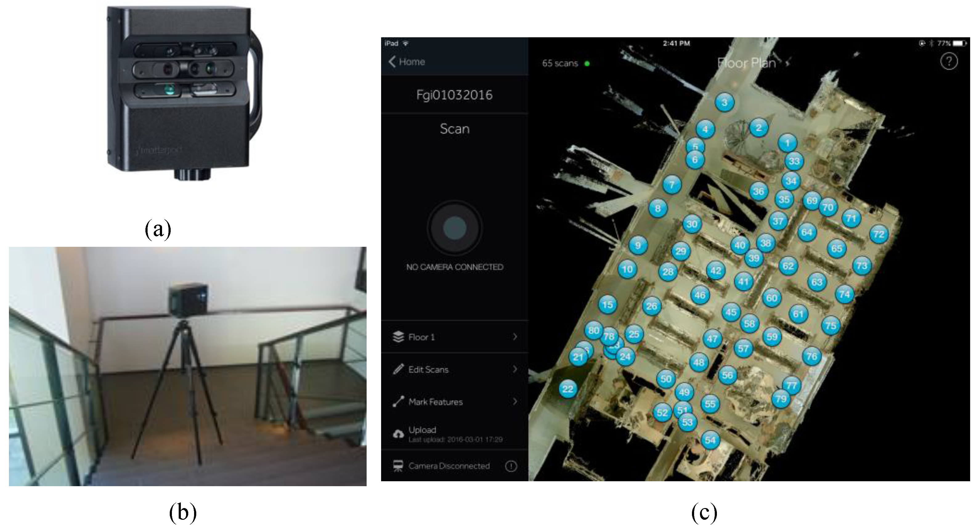
2.1. Matterport
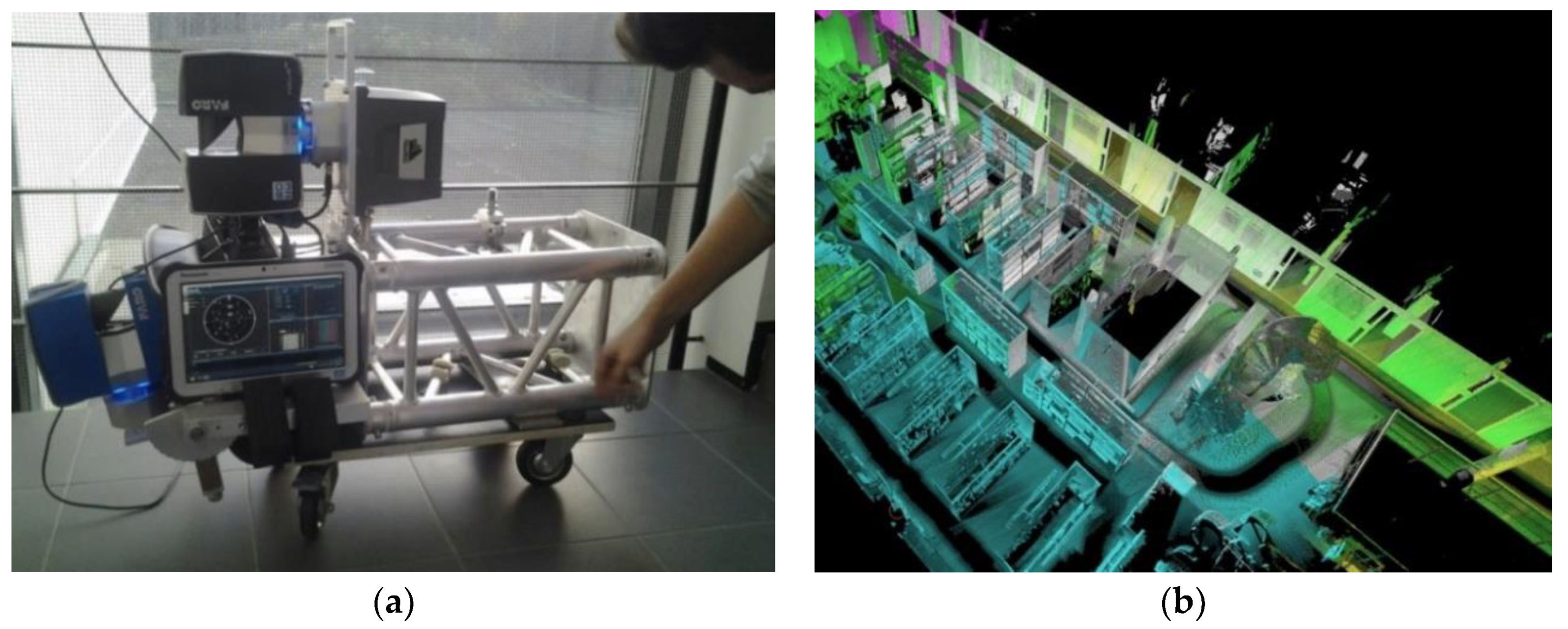
2.2. SLAMMER
3. Material and Methods
3.1. The First Test: An L Corridor
3.2. The Secnond Test: Three SLAM Based Indoor Mapping Solutions Comparison
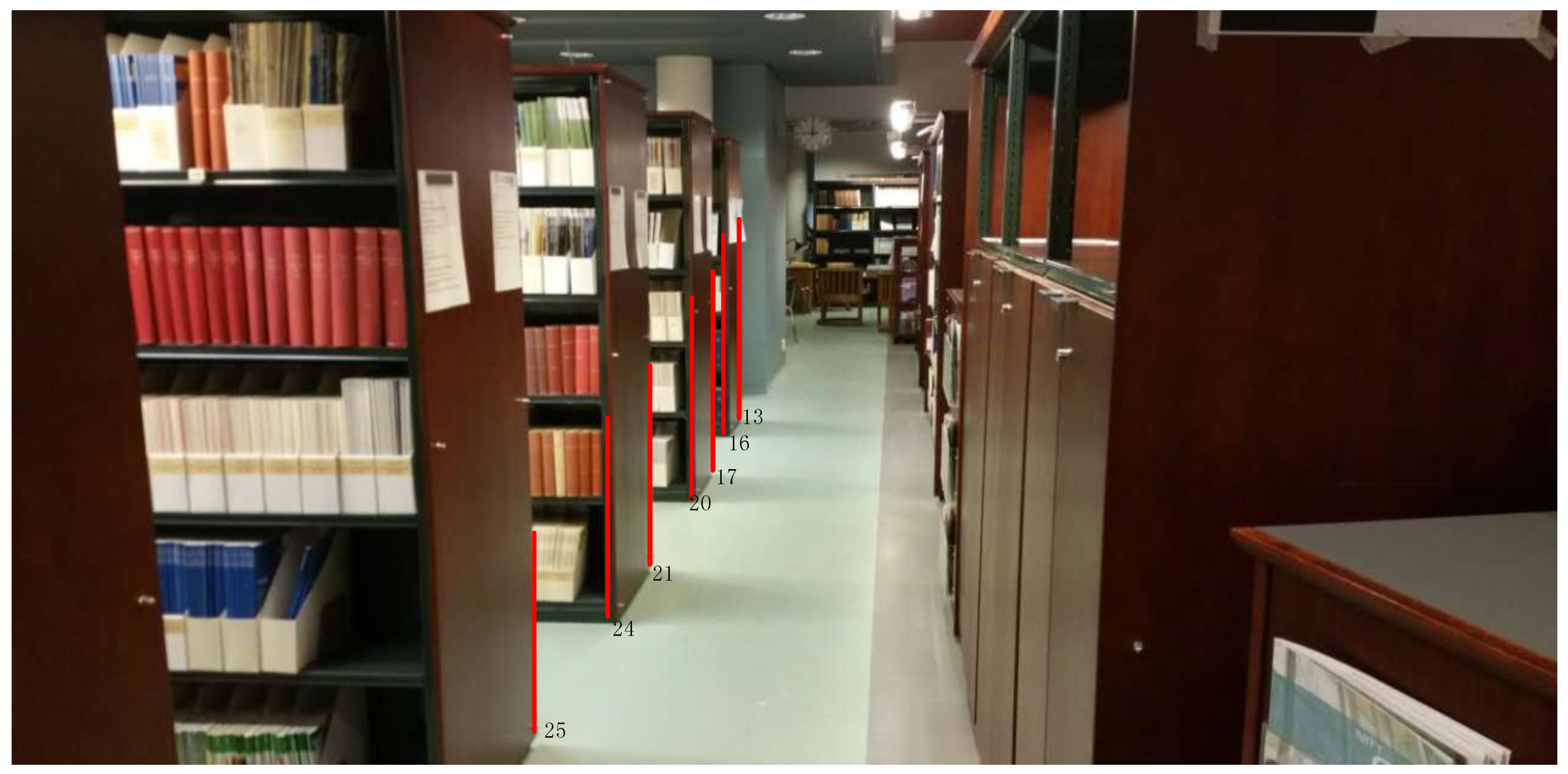
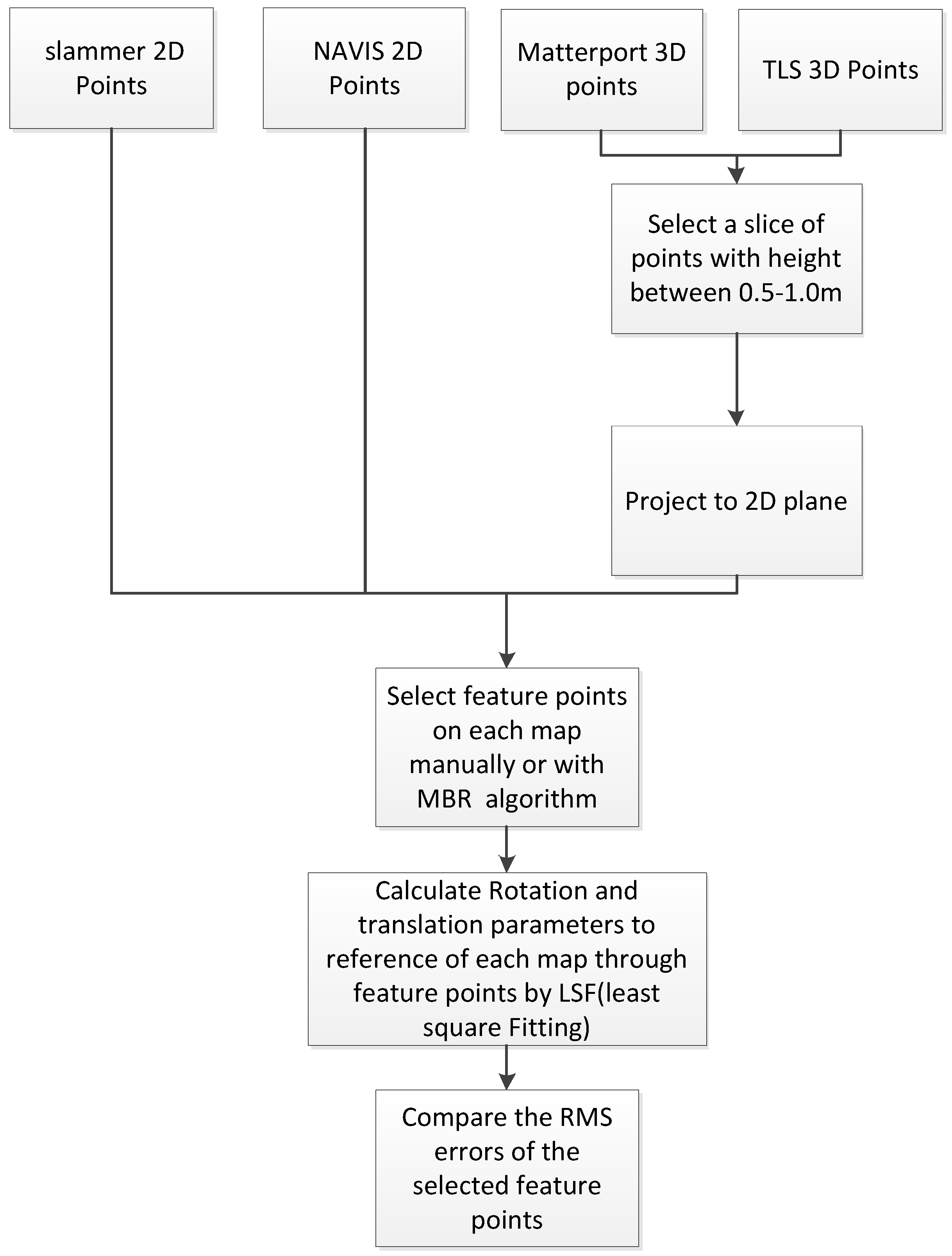
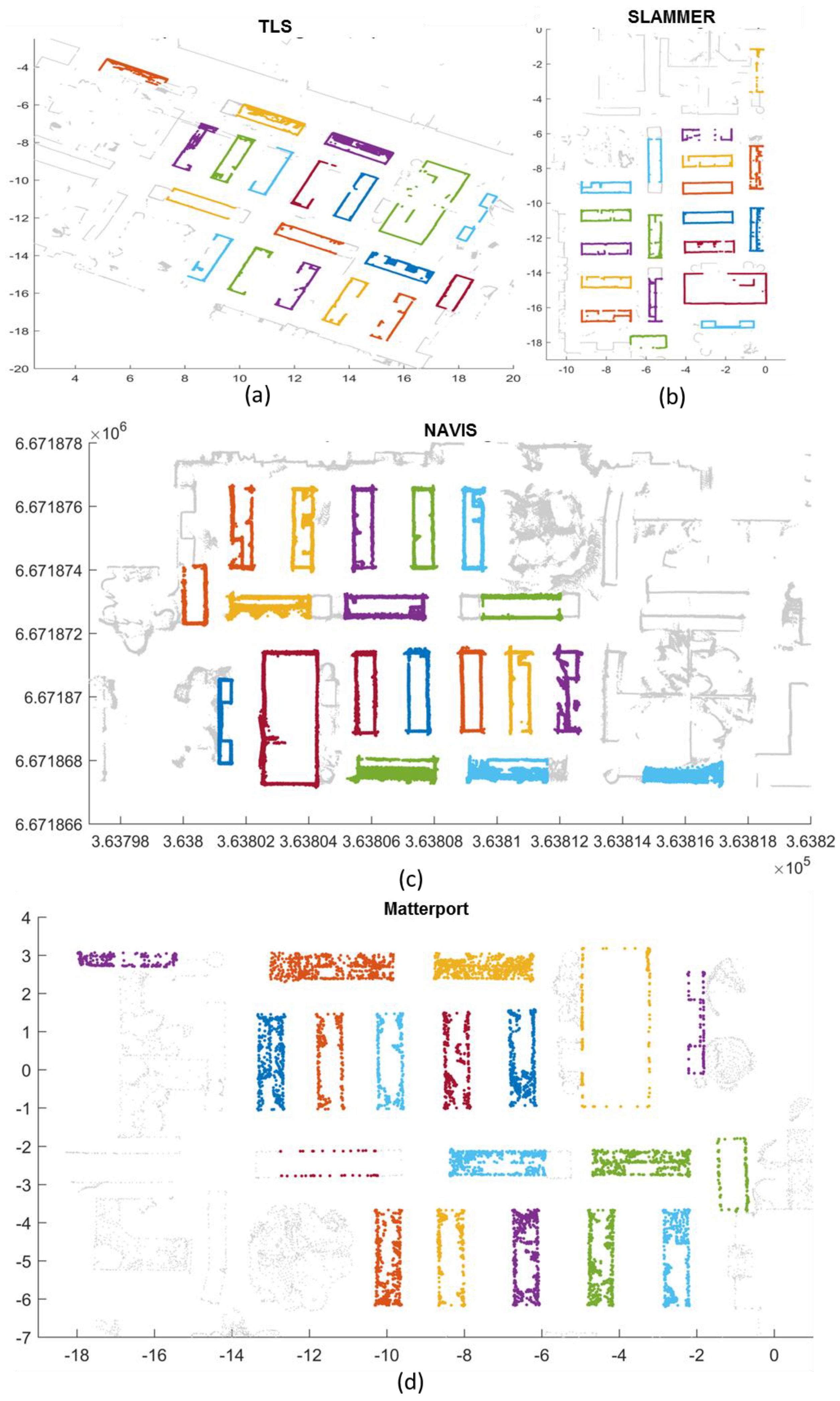
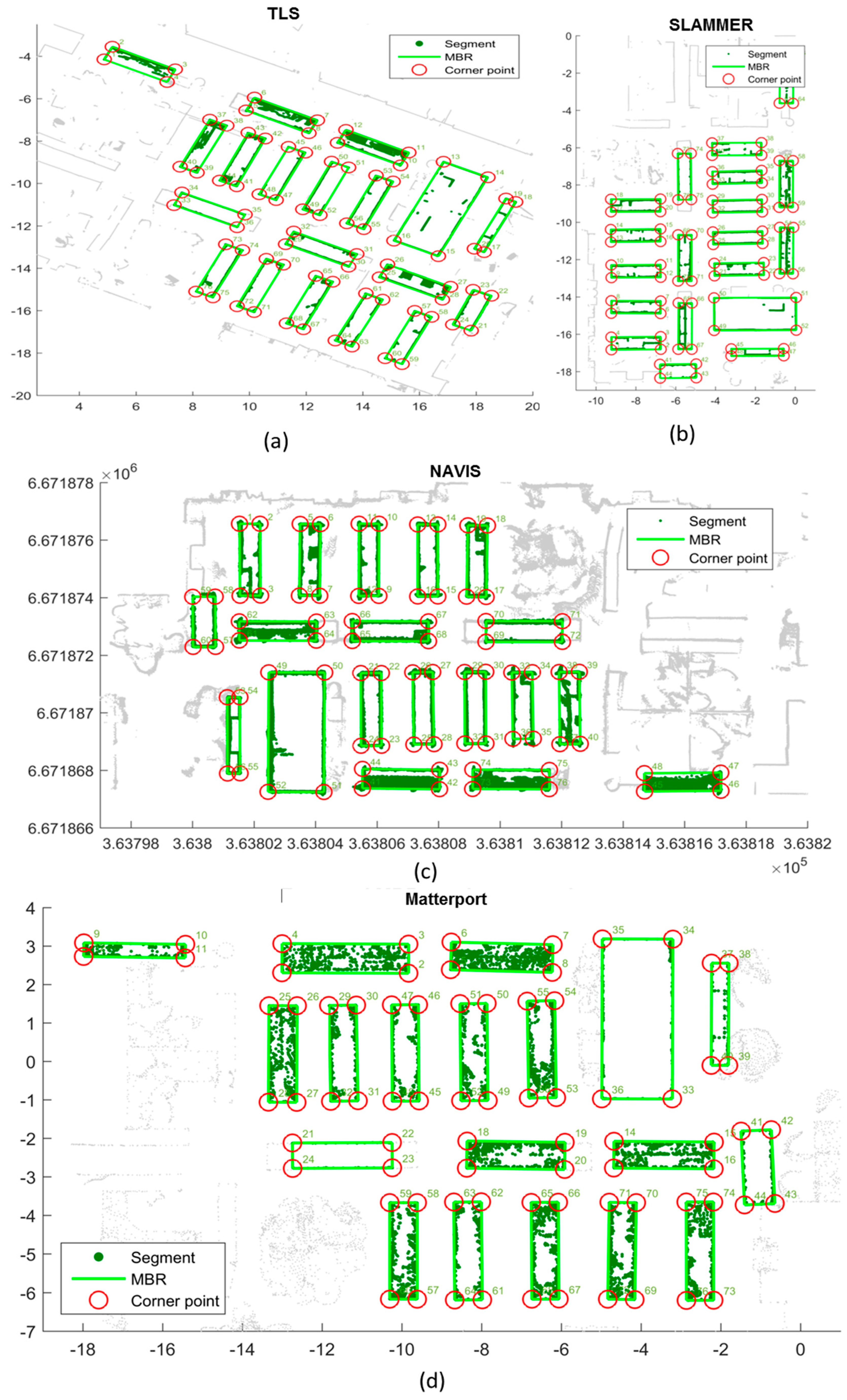
3.2.1. Feature Point Selection Method
- (1)
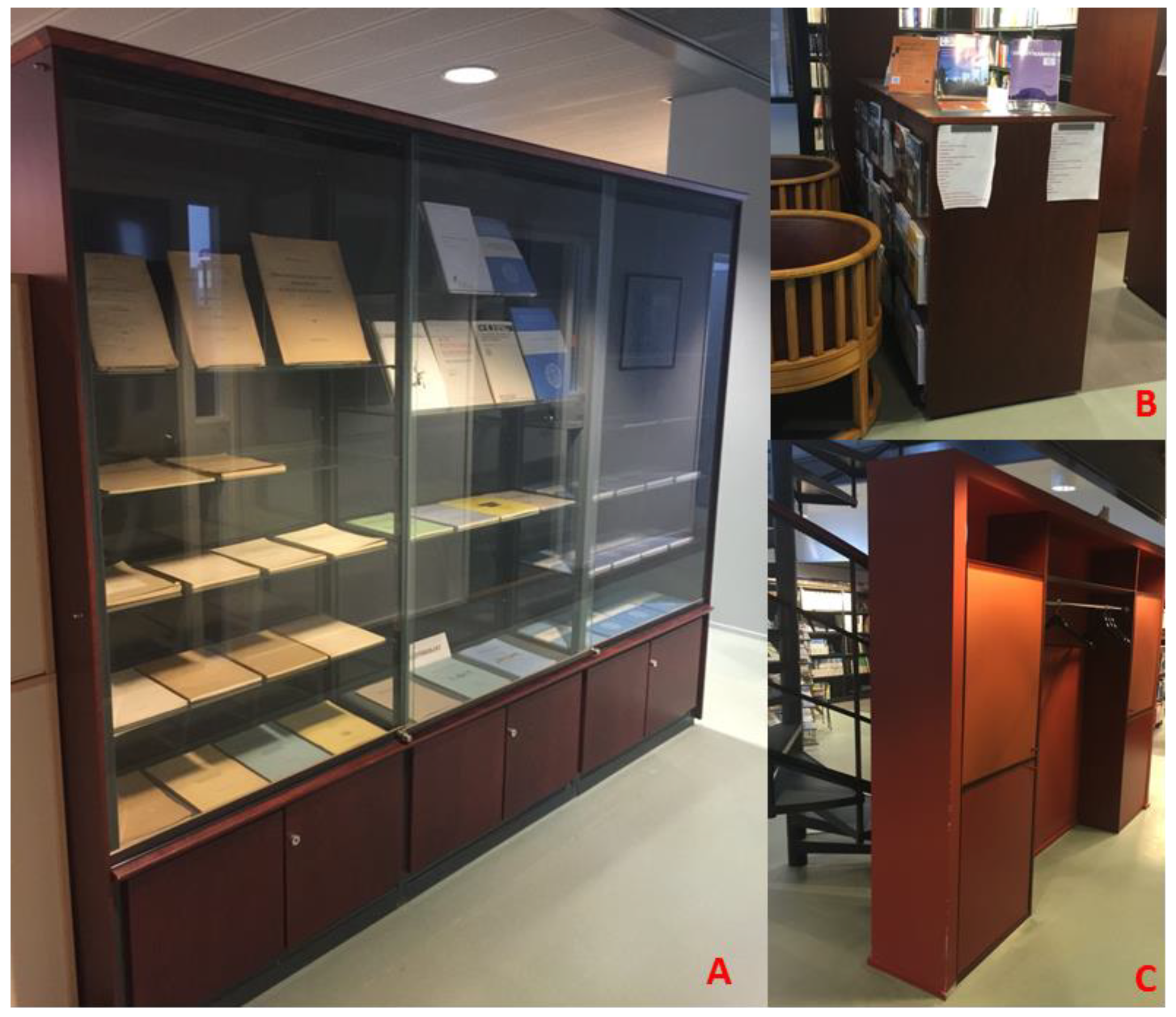
- Firstly, interactively segmentation is adopted to select the “area of interest”. Only the point cloud within the area of interest will be used for matching processing. The major reason for utilizing manually segmentation for indoor laser scanning was the accuracy demand of the results. Certain number of “false” point cloud was generated because of reflection of indoor glass-like objects, such as glass of a book cabinet, or polished metal surfaces.
- (2)
- A MBR algorithm was utilized to detect the rectangle shape within each area of interest.
- (3)
- The corner of rectangle can be extracted from the matched result. The extracted corners were then re-examined by an outlier detector to filter out the mismatched results and honestly evaluate the mapping accuracy, and the threshold of the outlier detector is 0.1 m.
3.2.2. Registration
4. Results and Discussion
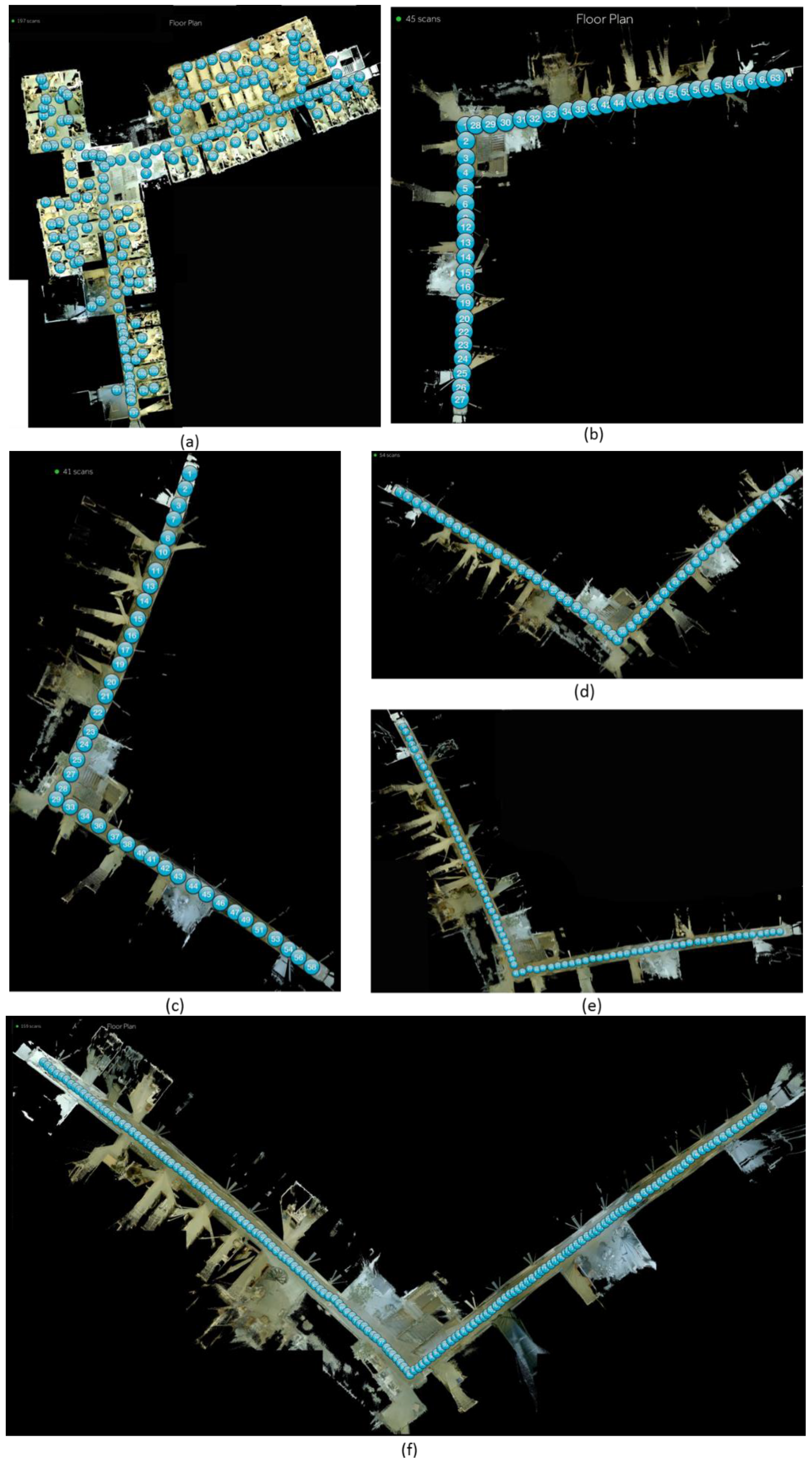
4.1. The First Scene: The L Shape Corridor
- The less the distance between neighboring scan, the more the total scan number is and the longer scan time is needed. The approximate coverage for the Matterport sensor is approximate 150 m2/h to 60 m2/h.
- The fail scan number and fail rate decrease when the distance between the neighboring scan decreases which implies that the density of scan effects the final mapping results. It has been addressed that the fail scan essentially increases the scan time.
- The manual selection of matched scans is efficient to mitigate the fail scan, however, it is only employed in a matrix measuring mode like Figure 6a presents where there is more than 1 neighboring scan to match. And it is not suitable for a linear measuring mode as T2–T6 surveys adopted where only one previous measurement can be utilized for matching.
4.1.1. Matterport is a SLAM
4.1.2. Mapping Trajectory Influence the Final Result
4.1.3. Optimal Parameter is Feasible for Matterport Indoor Mapping
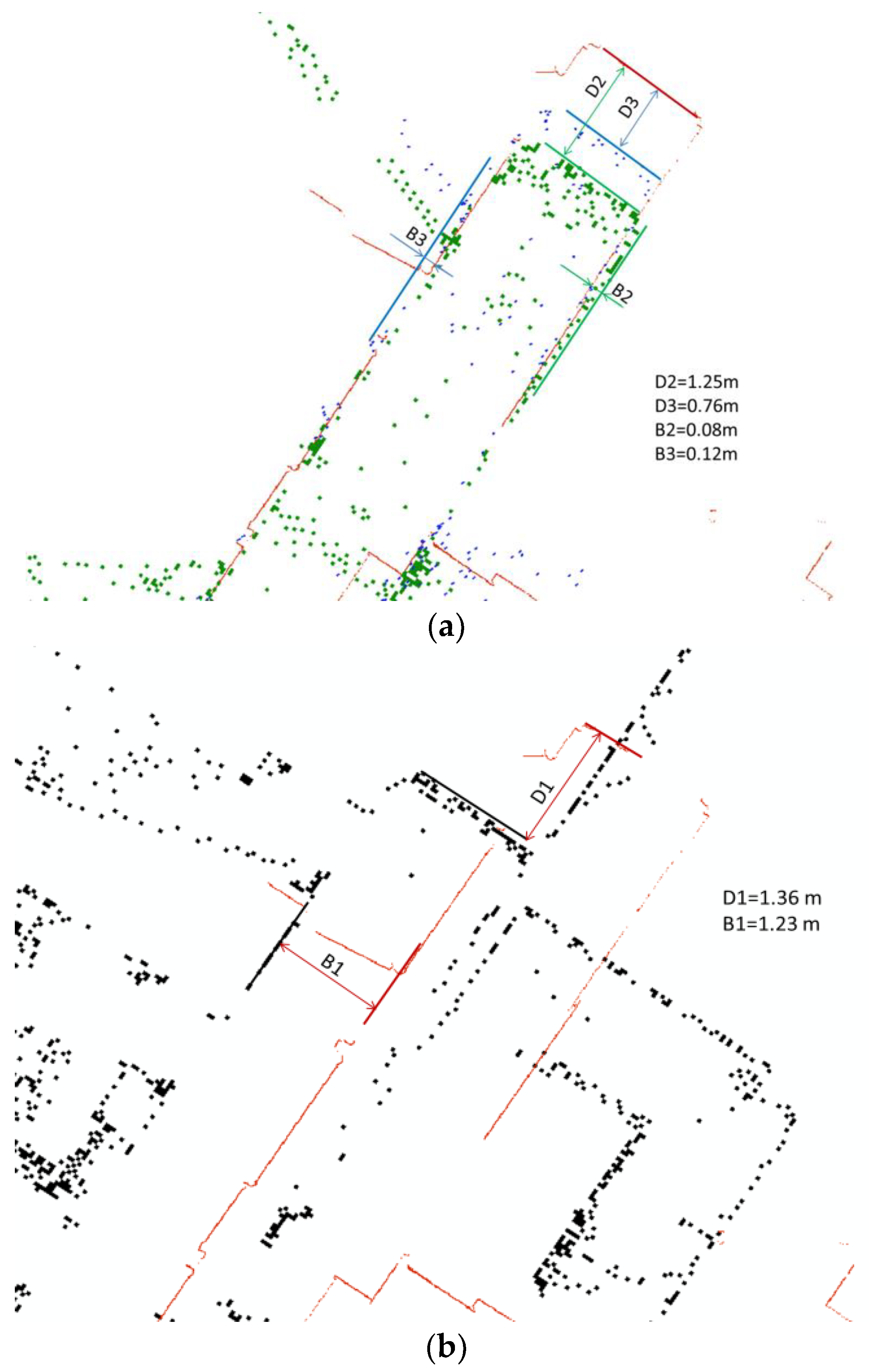
- The corner area of the corridor which contains a lot of contracture made of glass as Figure 9 presents. The reflection characteristics of the surface of glass made objects might bias the head estimation of the matching processing.
- No texture is attached with glass, with less feature, the accuracy of the matching processing might degrade.
- The 3-floor height glass wall in south front of the corner and the glass entrance of north front of the corner (Figure 9a) will introduce direct sunlight during the survey campaigns which might mislead the heading estimation error, and this should be avoided based on user manual recommendation. It is impractical to use large shades or drapes to block all nature light source during the survey.
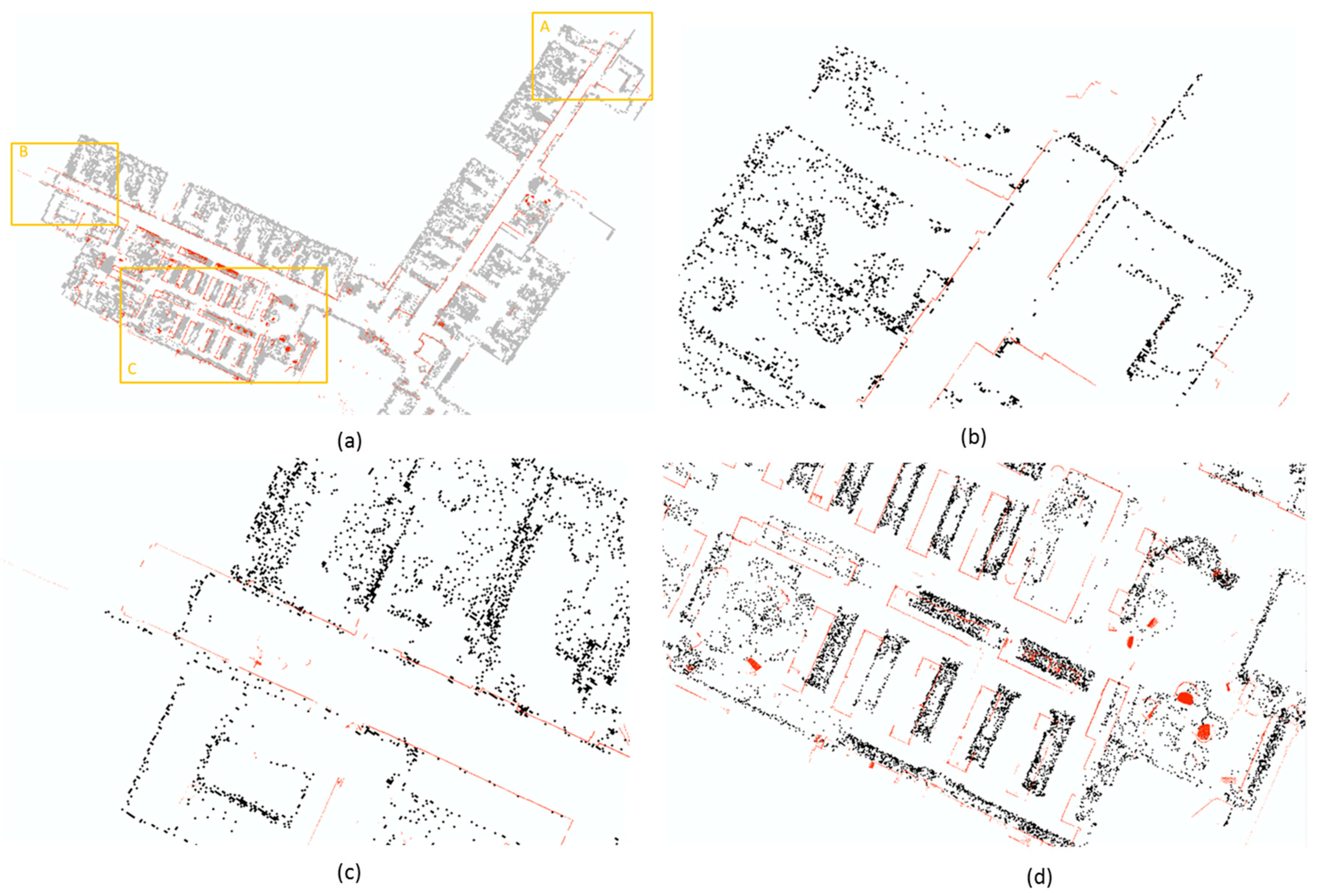
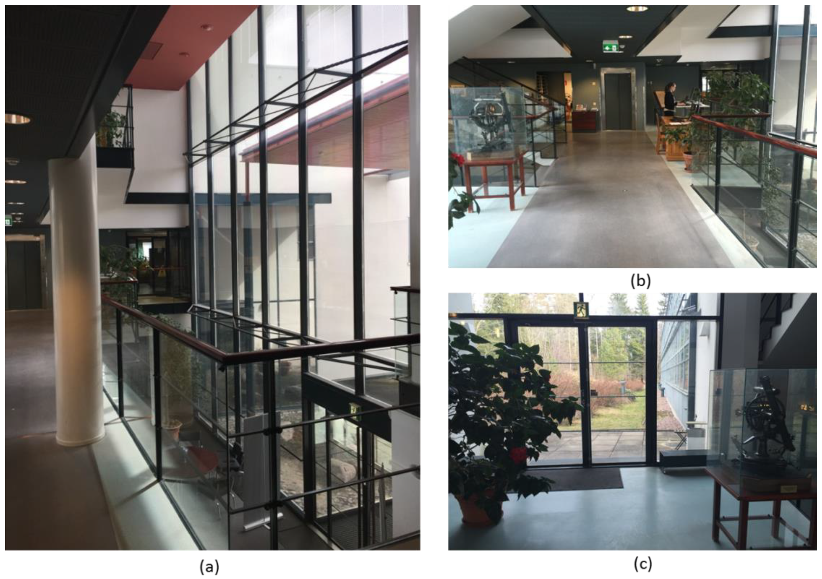
4.2. The Second Scene: An Open Style Library in FGI
4.2.1. Accuracy Evaluation with Interactively Selected Feature Points
4.2.2. Accuracy Evaluation with Feature Points Selected by MBRs
- (1)
- three SLAM-based indoor mapping technologies can all generate centimeter accuracy mapping result within a medium size managed indoor environment;
- (2)
- indoor mapping accuracy can be promoted by increasing the range accuracy of the adopt LiDAR or decreasing the footprint size of laser beam. by comparing the results of the SLAMMER and the NAVIS; the explanation is with more accurate measurement, the matching accuracy between continuous scan can be improved, and with smaller footprint laser beam, the measurement noise will also decrease, which results in the better mapping result;
- (3)
- Matterport is a reliable tool to generate 3D indoor model. However, extra labor is needed to filter out the mismatched feature points to produce a credible 2D map. Also the mapping accuracy is slightly worse than other two LiDAR based solutions.
5. Conclusions
Author Contributions
Funding
Acknowledgments
Conflicts of Interest
References
- Chen, R.; Chu, T.; Liu, K.; Liu, J.; Chen, Y. Inferring human activity in mobile devices by computing multiple contexts. Sensors 2015, 15, 21219–21238. [Google Scholar] [CrossRef] [PubMed]
- Mautz, R. Indoor Positioning Technologies. Ph.D. Thesis, ETH Zürich, Zürich, Switzerland, February 2012. [Google Scholar]
- Al Nuaimi, K.; Kamel, H. A survey of indoor positioning systems and algorithms. In Proceedings of the 2011 International Conference on Innovations in Information Technology (IIT), Abu Dhabi, UAE, 25–27 April 2011; IEEE: Piscataway, NJ, USA; pp. 185–190. [Google Scholar]
- Chen, Y.; Chen, R.; Pei, L.; Kröger, T.; Kuusniemi, H.; Liu, J.; Chen, W. Knowledge-based error detection and correction method of a multi-sensor multi-network positioning platform for pedestrian indoor navigation. In Proceedings of the 2010 IEEE/ION Position, Location and Navigation Symposium (PLANS), Indian Wells, CA, USA, 4–6 May 2010; IEEE: Piscataway, NJ, USA. [Google Scholar]
- Shi, G.; Ming, Y. Survey of indoor positioning systems based on ultra-wideband (UWB) technology. In Wireless Communications, Networking and Applications; Springer India: New Delhi, India, 2016; pp. 1269–1278. [Google Scholar]
- Gu, Y.; Lo, A.; Niemegeers, I. A survey of indoor positioning systems for wireless personal networks. IEEE Commun. Surv. Tutor. 2009, 11, 13–32. [Google Scholar] [CrossRef]
- Chen, R.; Chen, W.; Chen, X.; Zhang, X.; Chen, Y. Sensing walking strides using EMG signal for pedestrian navigation. GPS Solut. 2011, 15, 161–170. [Google Scholar] [CrossRef]
- Liu, H.; Darabi, H.; Banerjee, P.; Liu, J. Survey of wireless indoor positioning techniques and systems. IEEE Trans. Syst. Man Cybern. Part C: Appli. Rev. 2007, 37, 1067–1080. [Google Scholar] [CrossRef]
- Zlatanova, S.; Sithole, G.; Nakagawa, M.; Zhu, Q. Problems in indoor mapping and modelling. In Acquisition and Modelling of Indoor and Enclosed Environments 2013; ISPRS: Freiburg, Germany, 2013; Volume XL-4/W4. [Google Scholar]
- Thrun, S.; Leonard, J.J. Simultaneous localization and mapping. In Springer Handbook of Robotics; Springer: Berlin/Heidelberg, Germany, 2008; pp. 871–889. [Google Scholar]
- Bosse, M.; Zlot, R. Map matching and data association for large-scale two-dimensional laser scan-based SLAM. Int. J. Robot. Res. 2008, 27, 667–691. [Google Scholar] [CrossRef]
- Bowyer, K.W.; Chang, K.; Flynn, P. A survey of approaches and challenges in 3D and multi-modal 3D + 2D face recognition. Comput. Vis. Image Understand. 2006, 101, 1–15. [Google Scholar] [CrossRef]
- Zhang, J.; Singh, S. Loam: Lidar odometry and mapping in real-time. In Proceedings of the Robotics: Science and Systems Conference (RSS), Berkeley, CA, USA, 12–16 July 2014; pp. 109–111. [Google Scholar]
- Khoshelham, K.; Elberink, S.O. Accuracy and resolution of kinect depth data for indoor mapping applications. Sensors 2012, 12, 1437–1454. [Google Scholar] [CrossRef] [PubMed]
- Henry, P.; Krainin, M.; Herbst, E.; Ren, X.; Fox, D. RGB-D mapping: Using depth cameras for dense 3D modeling of indoor environments. In the 12th International Symposium on Experimental Robotics (ISER); Citeseer: Gaithersburg, MD, USA, 2010. [Google Scholar]
- Wikipedia. Simultaneous Localization and Mapping. Available online: https://en.wikipedia.org/wiki/Simultaneous_localization_and_mapping (accessed on 23 March 2016).
- Mur-Artal, R.; Montiel, J.M.M.; Tardos, J.D. ORB-SLAM: A versatile and accurate monocular SLAM system. IEEE Trans. Robot. 2015, 31, 1147–1163. [Google Scholar] [CrossRef]
- Engel, J.; Schöps, T.; Cremers, D. LSD-SLAM: Large-scale direct monocular SLAM. In Proceedings of the European Conference on Computer Vision, Zurich, Switzerland, 6–12 September 2014; pp. 834–849. [Google Scholar]
- Forster, C.; Pizzoli, M.; Scaramuzza, D. SVO: Fast semi-direct monocular visual odometry. In Proceedings of the 2014 IEEE International Conference on Robotics and Automation (ICRA), Hong Kong, China, 31 May–7 June 2014; pp. 15–22. [Google Scholar]
- Mueggler, E.; Rebecq, H.; Gallego, G.; Delbruck, T.; Scaramuzza, D. The event-camera dataset and simulator: Event-based data for pose estimation, visual odometry, and SLAM. Int. J. Robot. Res. 2017, 36, 142–149. [Google Scholar] [CrossRef]
- Weikersdorfer, D.; Adrian, D.B.; Cremers, D.; Conradt, J. Event-based 3D SLAM with a depth-augmented dynamic vision sensor. In Proceedings of the 2014 IEEE International Conference on Robotics and Automation (ICRA), Hong Kong, China, 31 May–7 June 2014; pp. 359–364. [Google Scholar]
- Besl, P.J.; McKay, N.D. Method for registration of 3-D shapes. In Robotics-DL Tentative; International Society for Optics and Photonics: San Diego, CA, USA, 1992; pp. 586–606. [Google Scholar]
- Censi, A. An ICP variant using a point-to-line metric. In Proceedings of the IEEE International Conference on Robotics and Automation (ICRA), Pasadena, CA, USA, 18–23 May 2008; pp. 19–25. [Google Scholar]
- Pathak, K.; Birk, A.; Vaskevicius, N.; Pfingsthorn, M.; Schwertfeger, S.; Poppinga, J. Online three dimensional SLAM by registration of large planar surface segments and closed form pose graph relaxation. J. Field Robot. 2010, 27, 52–84. [Google Scholar] [CrossRef]
- Lau, B.; Sprunk, C.; Burgard, W. Efficient grid-based spatial representations for robot navigation in dynamic environments. Robot. Auton. Syst. 2013, 61, 1116–1130. [Google Scholar] [CrossRef]
- Hornung, A.; Wurm, K.M.; Bennewitz, M.; Stachniss, C.; Burgard, W. OctoMap: An efficient probabilistic 3D mapping framework based on octrees. Auton. Robots 2013, 34, 189–206. [Google Scholar] [CrossRef]
- Olson, E. Real-time correlative scan matching. In Proceedings of the 2009 IEEE International Conference on Robotics and Automation (ICRA’09), Kobe, Japan, 12–17 May 2009; pp. 4387–4393. [Google Scholar]
- Pomerleau, F.; Colas, F.; Siegwart, R. A review of point cloud registration algorithms for mobile robotics. Found. Trends Robot. 2015, 4, 1–104. [Google Scholar] [CrossRef]
- Fuentes-Pacheco, J.; Ruiz-Ascencio, J.; Rendón-Mancha, J.M. Visual simultaneous localization and mapping: A survey. Artif. Intell. Rev. 2015, 43, 55–81. [Google Scholar] [CrossRef]
- Forster, C.; Zhang, Z.; Gassner, M.; Werlberger, M.; Scaramuzza, D. Svo: Semidirect visual odometry for monocular and multicamera systems. IEEE Trans. Robot. 2017, 33, 249–265. [Google Scholar] [CrossRef]
- Hess, W.; Kohler, D.; Rapp, H.; Andor, D. Real-time loop closure in 2D LIDAR SLAM. In Proceedings of the IEEE International Robotics and Automation Conference (ICRA), Stockholm, Sweden, 16–21 May 2016; pp. 1271–1278. [Google Scholar]
- Whelan, T.; Kaess, M.; Leonard, J.J.; McDonald, J. Deformation-based loop closure for large scale dense RGB-D SLAM. In Proceedings of the IEEE/RSJ International Intelligent Robots and Systems Conference (IROS), Tokyo, Japan, 3–7 November 2013; pp. 548–555. [Google Scholar]
- Alismail, H.; Baker, L.D.; Browning, B. Continuous trajectory estimation for 3D SLAM from actuated lidar. In Proceedings of the IEEE International Robotics and Automation Conference (ICRA), Hong Kong, China, 31 May–7 June 2014; pp. 6096–6101. [Google Scholar]
- Tang, J.; Chen, Y.; Kukko, A.; Kaartinen, H.; Jaakkola, A.; Khoramshahi, E.; Hyyppä, H. SLAM-aided stem mapping for forest inventory with small-footprint mobile LiDAR. Forests 2015, 6, 4588–4606. [Google Scholar] [CrossRef]
- Hewitt, R.A.; Marshall, J.A. Towards intensity-augmented SLAM with LiDAR and ToF sensors. In Proceedings of the IEEE/RSJ International in Intelligent Robots and Systems Conference (IROS), Hamburg, Germany, 28 September–2 October 2015; pp. 1956–1961. [Google Scholar]
- Kohlbrecher, S.; Von Stryk, O.; Meyer, J.; Klingauf, U. A flexible and scalable slam system with full 3d motion estimation. In Proceedings of the 2011 IEEE International Symposium on Safety, Security, and Rescue Robotics (SSRR), Kyoto, Japan, 1–5 November 2011; pp. 155–160. [Google Scholar]
- Kaijaluoto, R. Precise Indoor Localization for Mobile Laser Scanner. Master’s Thesis, Aalto University, Espoo, Finland, 2015. [Google Scholar]
- Kaijaluoto, R.; Kukko, A.; Hyyppä, J. Precise indoor localization for mobile laser scanner. In Proceedings of the Indoor-Outdoor Seamless Modelling, Mapping and Navigation, Tokyo, Japan, 21–22 May 2015; Volume XL-4/W5. 6 pages. [Google Scholar]
- Konolige, K.; Grisetti, G.; Kümmerle, R.; Burgard, W.; Limketkai, B.; Vincent, R. Efficient sparse pose adjustment for 2d mapping. In Proceedings of the 2010 IEEE/RSJ International Conference on Intelligent Robots and Systems (IROS), Menlo Park, CA, USA, 18–22 October 2010; pp. 22–29. [Google Scholar]
- Tang, J.; Yu, T.; Chen, Y.; Liu, J. An approach of dynamic object removing for indoor mapping based on UGV SLAM. Sens. Transducers J. 2015, 190, 40–46. [Google Scholar]
- Tang, J.; Chen, Y.; Chen, L.; Liu, J.; Hyyppä, J.; Kukko, A.; Kaartinen, H.; Hyyppä, H.; Chen, R. Fast fingerprint database maintenance for indoor positioning based on UGV SLAM. Sensors 2015, 15, 5311–5330. [Google Scholar] [CrossRef] [PubMed]
- Tang, J.; Chen, Y.; Jaakkola, A.; Liu, J.; Hyyppä, J.; Hyyppä, H. NAVIS-An UGV indoor positioning system using laser scan matching for large-area real-time applications. Sensors 2014, 14, 11805–11824. [Google Scholar] [CrossRef] [PubMed]
- Tang, J.; Chen, Y.; Niu, X.; Wang, L.; Chen, L.; Liu, J.; Shi, C.; Hyyppä, J. LiDAR scan matching aided inertial navigation system in GNSS-denied environments. Sensors 2015, 15, 16710–16728. [Google Scholar] [CrossRef] [PubMed]
- Matterport 3D Capture App 2.0 User Guide. Available online: http://matterport.com/wp-content/uploads/2014/10/Matterport-3D-Capture-App-2.0-User-Guide.pdf (accessed on 1 March 2016).
- Wood, J. Minimum bounding rectangle. In Encyclopedia of GIS; Springer: New York, NY, USA, 2008; pp. 660–661. [Google Scholar]
- Quigley, M.; Gerkey, B.; Conley, K.; Faust, J.; Foote, T.; Leibs, J.; Berger, E.; Wheeler, R.; Ng, A.Y. ROS: An open-source Robot Operating System. In Proceedings of the Open-Source Software Workshop of the International Conference on Robotics and Automation (ICRA), Kobe, Japan, 12–17 May 2009. [Google Scholar]
- Available online: https://www.hokuyo-aut.jp/02sensor/07scanner/utm_30lx_ew.html (accessed on 1 March 2016).
- Xsens, MTi User Manual; Revision E; Xsens Technologies B.V.: Enschede, The Netherlands, 2014.
- Mikhail, E.M.; Ackerman, F. Observations and Least Squares; Donnely, D., Ed.; Harper and Row: New York, NY, USA, 1976. [Google Scholar]
- Chen, Y.; Jiang, C.; Zhu1, L.; Tang, J.; Kaartinen, H.; Hyyppä, J.; Hyyppä, H.; Chen, R.; Pei, L. SLAM based indoor mapping comparison: Mobile or terrestrial? In Proceedings of the IEEE Ubiquitous Positioning, Indoor Navigation and Location-Based Services Conference, Wuhan, China, 22–23 March 2018. accepted and to be published. [Google Scholar]


| Laser Scanner (120S/X330) | |
| Range | 150 m/300 m |
| Wavelength | 905 nm/1550 nm |
| Field of View | 305 degrees |
| Max. measurement rate | 976k point/s |
| Profile rate | 30–97 Hz |
| Angular resolution | 0.157 mrad |
| Range error | ±2 mm |
| Ranging noise | 0.95–2.2 mm |
| IMU | |
| Gyro Technology | Fiber Optics Gyros |
| Data Rate | 200 Hz |
| Gyro Bias | <1.0 deg/h |
| Angular random walk | 0.05 degree/ |
| Attitude Accuracy | Roll:0.005 degree |
| Pitch: 0.005 degree | |
| Heading 0.008 degree | |
| Time accuracy | 20 ns |
| Weight | 4.25 kg + 5.2 kg + 5.2 kg + tablet and frame |
| Laser Scanner | |
| Range | 0.1–60 m |
| Wavelength | 905 nm |
| Field of View | 270° |
| Measurement rate | 43,200 points/s |
| Profile rate | 40 Hz |
| Angular resolution | 0.25° |
| Range error | ±30 mm |
| Ranging noise | 10 mm |
| IMU | |
| Gyro Technology | MEMS |
| Data Rate | 100 Hz |
| Gyro Bias Stability | 10 degree/h |
| Angular Random Walk | 3 |
| Velocity Random Walk (VRW) | 0.12 |
| Attitude Accuracy | Roll: 0.3 degree |
| Pitch: 0.3 degree | |
| Heading 1 degree | |
| Total Weight | 270 g + 58 g + laptop and frame |
| Surveying Campaign | Distance between Neighboring Scan | Start Point | Total Scan | Fail Scan | Fail Rate | Scan Time |
|---|---|---|---|---|---|---|
| T1 | 0.5–3 m | Corner | 197 | 0 * | 0% | 195 min |
| T2 | 2 m | Corner | 41 | 17 | 29.3% | 95 min |
| T3 | 2 m | End | 45 | 18 | 28.6% | 102 min |
| T4 | 0.5 m | End | 159 | 0 | 0% | 148 min |
| T5 | 1 m | End | 81 | 2 | 2.4% | 87 min |
| T6 | 1.5 m | End | 54 | 5 | 8.5% | 60 min |
| Surveying Campaign | Distance between Neighboring Scan | Start Point | Bias Error | Heading Estimation Error | Distance Error |
|---|---|---|---|---|---|
| T2 | 2 m | Corner | 0.08 m | 0.11° | −1.25 m |
| T3 | 2 m | End | −0.12 m | −0.17° | −0.76 m |
| T1 | 0.5–3 m | Corner | −1.23 m | −1.76° | −1.36 m |
| Surveying Campaign | Distance between Neighboring Scans | Start Point | Bias Error | Heading Estimation Error | Distance Error |
|---|---|---|---|---|---|
| T2 | 2 m | Corner | 0.08 m | 0.11° | −1.25 m |
| T3 | 2 m | End | −0.12 m | −0.17° | −0.76 m |
| T4 | 0.5m | End | 1 m | 1.43° | −0.15 m |
| T5 | 1 m | End | 0.32 m | 0.46° | 0.15 m |
| T6 | 1.5 m | End | 0.80 m | 1.15° | −0.70 m |
| SLAMMER | NAVIS | Matterport | TLS | |
|---|---|---|---|---|
| Point | 4.29 M | 1.01 M | 12,098 | 3.7 M |
| TLS | SLAMMER | NAVIS | MATTERPORT | |
|---|---|---|---|---|
| RMSE (m) | - | 0.020 | 0.037 | 0.042 |
| Feature points | 91 | 91 | 90 | 84 |
| Detection rates | - | 100% | 98.9% | 92.3% |
| TLS | SLAMMER | NAVIS | MATTERPORT | |
|---|---|---|---|---|
| Extracted feature points | 76 | 76 | 76 | 76 |
| Effective feature point | 76 | 76 | 74 | 72 |
| Detection rate | - | 100% | 97.3% | 94.7% |
| RMSE (m) | - | 0.017 | 0.032 | 0.047 |
| SLAMMER | NAVIS | Matterport | |
|---|---|---|---|
| Effective Range | 150 m | 0.1–60 m | 12 feet between scans |
| IMU | Tactical-grade IMU | Consumer-grade IMU | None |
| Mobility | Yes | Yes | No |
| Texture | No | No | Yes |
| Measure with disturbance | Yes | Yes | No |
| Cost | High | Low | Low |
| Real Time Performance | Yes (real time mode with lower mapping accuracy) | Yes | No |
| Scanning time | Short | Short | Long |
| Range Sensor | FARO Focus3D 120S | Hokuyo UTM-30LX-EW | Kinect type depth camera |
| Footprint size (at 10 m) | 4.2 mm | >130 mm | - |
| Range Accuracy | 2 mm | 3 cm | - |
| Initialization outdoor | Yes | No | No |
| Synchronization | Hardware | Software | - |
| Dynamic Object Filter | No | Yes | No |
| Point Cloud Density | High | Medium | Low |
| Data Collecting Efficiency | High (several minutes for FGI library) | High (several minutes for FGI library) | Low (2 h for FGI library) |
| Weight | High | Low | Low |
| Power Consumption | High | Low | Low |
| Operator | trained operator | trained operator | untrained operator |
© 2018 by the authors. Licensee MDPI, Basel, Switzerland. This article is an open access article distributed under the terms and conditions of the Creative Commons Attribution (CC BY) license (http://creativecommons.org/licenses/by/4.0/).
Share and Cite
Chen, Y.; Tang, J.; Jiang, C.; Zhu, L.; Lehtomäki, M.; Kaartinen, H.; Kaijaluoto, R.; Wang, Y.; Hyyppä, J.; Hyyppä, H.; et al. The Accuracy Comparison of Three Simultaneous Localization and Mapping (SLAM)-Based Indoor Mapping Technologies. Sensors 2018, 18, 3228. https://doi.org/10.3390/s18103228
Chen Y, Tang J, Jiang C, Zhu L, Lehtomäki M, Kaartinen H, Kaijaluoto R, Wang Y, Hyyppä J, Hyyppä H, et al. The Accuracy Comparison of Three Simultaneous Localization and Mapping (SLAM)-Based Indoor Mapping Technologies. Sensors. 2018; 18(10):3228. https://doi.org/10.3390/s18103228
Chicago/Turabian StyleChen, Yuwei, Jian Tang, Changhui Jiang, Lingli Zhu, Matti Lehtomäki, Harri Kaartinen, Risto Kaijaluoto, Yiwu Wang, Juha Hyyppä, Hannu Hyyppä, and et al. 2018. "The Accuracy Comparison of Three Simultaneous Localization and Mapping (SLAM)-Based Indoor Mapping Technologies" Sensors 18, no. 10: 3228. https://doi.org/10.3390/s18103228
APA StyleChen, Y., Tang, J., Jiang, C., Zhu, L., Lehtomäki, M., Kaartinen, H., Kaijaluoto, R., Wang, Y., Hyyppä, J., Hyyppä, H., Zhou, H., Pei, L., & Chen, R. (2018). The Accuracy Comparison of Three Simultaneous Localization and Mapping (SLAM)-Based Indoor Mapping Technologies. Sensors, 18(10), 3228. https://doi.org/10.3390/s18103228