Abstract
Many fault detection methods have been proposed for monitoring the health of various industrial systems. Characterizing the monitored signals is a prerequisite for selecting an appropriate detection method. However, fault detection methods tend to be decided with user’s subjective knowledge or their familiarity with the method, rather than following a predefined selection rule. This study investigates the performance sensitivity of two detection methods, with respect to status signal characteristics of given systems: abrupt variance, characteristic indicator, discernable frequency, and discernable index. Relation between key characteristics indicators from four different real-world systems and the performance of two fault detection methods using pattern recognition are evaluated.
1. Introduction
Fault detection is a key status monitoring function that identifies the presence of faults in a system, and the times at which they occurred. Fault detection methods use pattern recognition with large datasets have been applied to various engineering areas [1] since these do not require any additional empirical knowledge to model a given system [2]. However, it is still not easy to extract meaningful patterns directly from the original datasets. For example, Hellerstein, Koutsoupias [3] demonstrated that the performance of several non-trivial pattern extraction and indexing algorithms degraded as the size of the given dataset increased. Therefore, data discretization methods have been used as a preprocessing step to reduce the dimensionality of the original dataset, while preserving the important information for pattern extraction [4,5,6]. These discretization methods commonly involve dividing the datasets into finite segments and converting each segment into an appropriate label [7]. Unsupervised discretization methods do not use the data to determine segment boundaries. Equal width discretization and equal frequency discretization are two typical unsupervised discretization methods that create continuous-valued attributes by creating a specified number of bins [8,9]. In contrast, supervised methods discretize data by considering the relations between the data values and the class information of the system. Entropy-based discretization methods is the typical supervised method, and it measures the purity of the information to determine boundaries that decrease the entropy at each interval. Maximum entropy [10] and minimum entropy [11] methods use the entropy of the information to determine suitable stopping criteria.
One issue with these methods is that the features that are extracted from the time domain are not always enough to distinguish between the no-fault and the fault states. For example, the amplitude of the time series shown in Figure 1 is the same throughout even though it includes both the no-fault state and the fault state. If the features that use the amplitude of the time series are identical in both states, it is difficult to discriminate between two states. Instead, the data show that the two states have different frequencies.
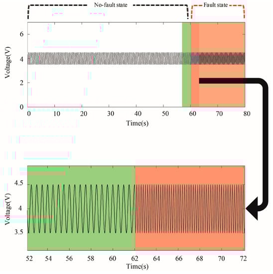
Figure 1.
Time series where the frequency changes when the state of the system changes.
Such characteristics appear in the acoustic and vibrational data that are usually collected from mechanical systems, such as rotors and bearings [12,13]. If a mechanical system has faults, then they usually generate a series of impact vibrations, and these appear with different frequencies [14]. Signal processing methods have been applied to such time series to measure and analyze the vibration responses, with the aim of detecting faults in the frequency domain [15,16,17]. Fast Fourier transforms and various of Time-frequency analysis methods are the representative signal processing methods for analyzing the frequency domain [18].
Several model-based fault detection methods using frequency features have been proposed. The performance of model-based fault detection, by nature, is dependent on a proposed system model itself. However, the operational outputs of many industrial systems are often different from the intended behaviors due to unknown disturbances, system degradation, and measurement noises [19]. Hence, observer-based approaches have been devised to combine a system model with residuals [20]. Recently, fault observer fuzzy models for complex nonlinear dynamic processes have been presented in finite-frequency domain [21,22,23].
Data-driven approaches have been develop to make fault status decisions by analyzing a large amount of historic data in the case of absence of any predefined system model [24]. Many studies have been made to discover fault patterns, i.e., particular time-frequency features, via various machine learning techniques [25,26,27,28]. Here, it is necessary to compose system status patterns by using either amplitude variation in time domain or frequency variation in frequency domain.
Therefore, the first objective of this study is to develop a pattern extraction method that discretizes the frequency components of multivariate data. In Section 2, the labels are defined using features in the frequency domain. The procedures for discretization and pattern extraction follow those of previous work that used time-domain features to construct labels [29].
The second objective of this study is to provide a guideline for selecting appropriate labels for fault pattern extraction via a comparison between the performance of different pattern extraction methods and the representative characteristics that they extract from the time series. In the process, several key characteristics indicators (KCIs) and an aggregated characteristic indicator is suggested. The guideline is also proposed regarding the type of labels that should be selected based on the key characteristics. The key characteristics of the time series and the experimental study are introduced in Section 3 and Section 4. The nomenclature regarding indices, parameters, and variables is summarized in Table 1.

Table 1.
Nomenclature.
2. Methodology
2.1. Frequency Variation-Based Discretized Time Series Generation
Conventional discretization methods downsize time series into a finite number of bins that preserve the temporal information of the original time series. Such methods have been applied to fault detection, owing to their efficiency in extracting patterns using discretized labels that are derived from statistical features of the discretized bins [5]. However, these methods assume that the statistically discernible features needed for fault detection exist in the time domain. In the case of vibrational systems, where the dominant features generally lie in the frequency domain; this means that the patterns for fault states and no-fault states cannot be distinguished. Therefore, we propose a new discretization method that uses frequency domain features as labels, following the systematic discretization method introduced in previous work [29]. The method is briefly described in the following section.
2.2. Discretization-Based Fault Pattern Extraction
The discretization-based fault pattern extraction method aims to extract a set of fault patterns from the training data of a given system for fault detection. Therefore, the information of no-fault state and fault state, namely fault time markers, are assumed to be given a priori. The method comprises three steps: label definition, label specification, and fault pattern extraction.
The label definition step involves estimating the distribution model of the time series, and dividing the given time series into a finite number of bins. Assume that a given time series is collected from a system containing sensors. Let be the data points in the time series gathered by the ith sensor and be a set of sensor data.
Then, the probability density function (PDF) is estimated to determine the distribution model of the given data set. The probability density function, , whose statistical characteristics are most similar to those of the dataset is determined by computing the optimal likelihood values between the histogram of the original datasets and the PDF candidates.
After that, a set of cut-points are generated using the set of segments, , and the discretization parameters , which determines the number of bins, and , which defines the size of the central bin that contains the centroid of . We used odd values for to generate balanced sets of labels where the probability density of each bin, except the center bin, was identical. After setting these parameters, a set of cut-points is derived from the data from each sensor, , followed by a set of labels . For instance, Figure 2 shows a procedure of the label definition step.
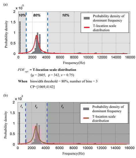
Figure 2.
An example of probability density function (PDF) estimation for a dominant frequency of microphone sensor data collected by the automotive buzz, squeak, and rattle (BSR) noise detection system. (a) of the sensor data, which follows a T-location scale distribution. The cut points of the dominant frequency, [1069 Hz, 4142 Hz] is derived with the user-defined discretization parameters, bin width, and the number of bins; (b) A set of labels [ is determined according to the number of cut points and the feature of each bin.
The label specification step divides the data into discrete segments and attaches the corresponding labels to them. A matrix consists of labeled segments are named as the discrete state vector, where the represents the label assigned to the sth segment. Here, the label for each segment is determined by its relative location of the average value of the amplitude. Then, is converted into a set of discrete state vector, :
To represent the state of the system in terms of the labels that are assigned to each sensor, m labels for a given time index, i.e., a column vector of D(X), are converted into event codes. The event codes are combination of all the possible discrete state vectors, where a total number is . The event codes are assigned into the set of discrete state vectors, which the composition of discrete state vectors is same. For instance, in Figure 3, we defined the first event code, as [], the second event code, as [], and so on. We assigned to the fifth set of discrete state vectors due to the same composition of discrete state vectors.
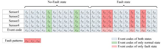
Figure 3.
An example of the fault pattern extraction procedure (dataset with four sensors): Each sensor data (Sensor 1, Sensor 2, Sensor 3, Sensor 4) has same length, and discretized into 24 segments. Meanwhile, a set of cut-points of each sensor data are derived by PDF estimation, followed by a set of labels . Then, designated labels in each column of four sensor data are converted into unique event codes, which are depicted as . As a result, are selected as fault patterns.
The set of fault patterns is composed of the event codes that only occur in fault states of the system, as Figure 3 shows. In other words, is the relative complement of in , where is the set of distinct event codes that occur in fault states and is the set of distinct event codes that occur in no-fault states. The method then determines the state of the given time series X depending on whether there is an element of in D(X).
As performance of the fault detection is determined as follows: the number of the fault states where a specific fault pattern is found. Herein, the label definitions play a key role in this scheme. In the next section, we propose a new label definition using the frequency-domain features to expand the coverage of the discretization method.
2.3. Dominant Frequency Extraction for Each Segment
Frequency components have been popularly used to fault detection, Fast Fourier transforms is one of methods to extract frequency components from the original sensor signals of the system [26]. However, in general, traditional FFTs require periodic and stationary datasets, and are not directly applicable to analyze the time dependent frequency variation of sensor signals, whereas many datasets of interests exhibit non-stationary characteristics [30]. Time-frequency analysis methods, such as short time Fourier transforms (STFTs) and wavelet transforms (WTs), have been suggested to analyze non-stationary signals by applying FFT to the segmented signals in each time window [18]. Therefore, we applied STFT in order to combine a time-frequency analysis into temporal discretization methods for label definition. Figure 4 shows an example of dominant frequency extraction for label definition in the frequency variation-based discretization procedure.
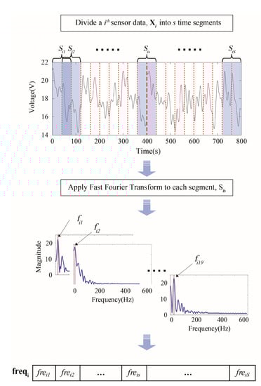
Figure 4.
Extraction of the dominant frequency in the time series.
Before defining the labels, the time series is divided into segments using the predetermined parameter, , which represents the size of the segment. The number of segments is therefore equivalent to , where is the number of data points in . If the segmentation process leaves a remainder, this is ignored on the basis that it does not contain a significant amount of information. For segmentation, we applied the sliding window method to preserve sequential information [31]. The sliding window overlap was set to half of the window size . The number of segments is therefore equivalent to . Let be segmented into the total segments, and then for a given window size and sliding window size , the set of data points in the sth time segment of the ith sensor, is given by:
The procedure is done with the window size of a time segment = 40 s, the sampling rate = 1 kHz, s = 19. , which iss ith sensor data, is divided into s segments, and FFT is applied to each segment for extracting the dominant frequency. Finally, a sequence of dominant frequency, is acquired.
We can now represent the overall sensor dataset and the time series from each sensor in terms of these sets of segments. The following label definition is now proposed. Let denote the Fourier coefficient of the sinusoid for the sth time segment signal of the ith sensor. We can obtain the Fourier coefficient by applying a FFT to , where the Fourier component .
Let denote the vector, and the Fourier matrix Wi for the ith sensor data is then defined as follows.
For the sake of simplicity, without a loss of generality, we employ the dominant frequency having the highest peak in the frequency spectrum as a key feature to characterize the inherent information in the frequency domain. The dominant frequency in the sth segment of the ith sensor data is denoted as Finally, a vector of dominant frequencies , is obtained from the , as follows.
2.4. Characterization of System Status Signals
The fault pattern extraction performance is highly affected by whether appropriate labels are selected to characterize the time series. To ensure that the labels are suitable, we need to determine the relation between the characteristic indicators for the collected signal and the fault pattern extraction performance. In this section, three KCIs are introduced to represent the characteristics of the time series of the given signal: abrupt variance (aVar) and discernibility index (DI) from the previous research, and discernable frequency (DF). Furthermore, we define CI as an aggregated characteristic index of DI and DF. We analyzed four datasets of multi-sensor signals and represented the main feature of each dataset by the three KCIs and the aggregated index CI. We discuss the relationships between fault detection performance and KCIs.
aVar was devised by multiplying a square sum of differences between adjacent data points to conventional variance for determining the magnitude of the abrupt and steady changes, and it is given by following equation [29].
In contrast, the DI measures the degree of statistical overlap between no-fault and fault states, as follows [29]:
where and represent the estimated PDFs for the sensor data x in the no-fault and the fault states respectively.
We further define the DF to represent the frequency similarity between fault and no-fault states in terms of the composition of the time-frequency components. Existing features in the frequency domain, such as the dominant frequency and power spectral density, cannot represent time-frequency characteristics of the data because they utilize a classical FFT [19]. The DF is therefore defined as follows.
and represent the estimated PDFs of the frequency of the ith sensor signal in the no-fault and the fault states respectively. Figure 5 shows an example DF calculation, giving a frequency similarity of 0.331.
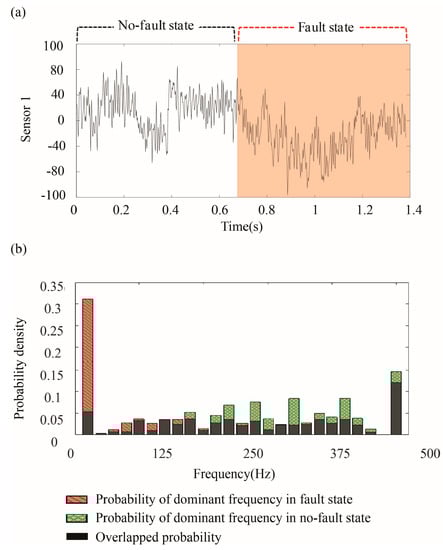
Figure 5.
Calculation of DF (DF = 0.331): (a) A sensor signal; and, (b) the probability density of dominant frequencies in the fault, the no-fault states, and the overlapped probability density between them.
The CI is further defined to simultaneously highlight the performance of the DI and DF for the given data set. It is calculated by multiplying the complement of the DI with the DF, as follows.
3. Computational Experiment
In this section, we evaluate the performance of the discretization-based fault pattern extraction method by considering both frequency and amplitude variation, and discuss the relationship between the KCIs of system status signals and performance of fault detection. The detailed description of the experimental data is listed in Table 2.
Table 2.
Description of experimental datasets.
Previous studies used a statistical representative sensor value and/or its linear trend in each time segment to construct a set of labels. We will call the fault patterns that are generated by the amplitude variation of sensor values as FP1, and those generated by the frequency variation of sensor values as FP2. The two pattern generation methods were applied to real-world datasets collected from four mechanical systems. The following subsections describe each system and provide brief information regarding the performance of pattern extraction with respect to the KCIs. The results are summarized in Table 3.
Table 3.
Fault detection performance and key characteristics indicators (KCIs) for the four datasets.
3.1. Laser Welding Monitoring Data
Laser welding monitoring data, shown in Figure 6a, were collected from a laser welding system, as shown in Figure 7. This system was originally developed to examine the relationship between the part-to-part gap of two galvanized steel sheets and the weldment quality of a joint. The system consisted of PRECITEC LWMTM (Precitec, Gaggenau, Germany) as a data acquisition device. The system used a IPG YLS 2000 AC fiber laser source (IPG Photonics, Oxford, MA, USA) with a maximum output discharge of 2 kW.
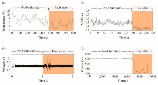
Figure 6.
Sensor data collected from four different systems having no-fault state and fault state: (a) temperature signals collected from the laser welding monitoring system; (b) MAP (Manifold Absolute Pressure) signals collected from the vehicle diagnostics simulator; (c) microphone sensor signals collected from the automotive BSR noise monitoring system; and, (d) sensor signals for turbocharger inlet temperature collected from the marine diesel engine.
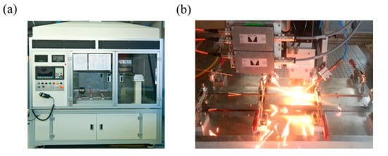
Figure 7.
Laser welding monitoring system: (a) Laser welding station and (b) PRECITEC laser welding monitoring sensors.
We controlled the gap between the galvanized steel sheet parts by inserting a conventional metal thickness gauge having thickness of 0.1 mm to 1.0 mm. The travelling path of the laser was defined as ascending direction. In this study, we generated five defective weldments by controlling the artificial gap (=0.5 mm) between specimens, and forty-five normal weldments without gap.
The computed KCIs are listed in Table 2, showing low aVar and DI but high DF and CI. By using FP1, we could detect all the five weld defects, while only two defects were identified by FP2.
3.2. Automotive Gasoline Engine Data
Automotive gasoline engine data, shown in Figure 6b, were collected from a vehicle diagnostics simulator, shown in Figure 8. The system consists of 40 sensors on SIRIUS-II engine (Hyundai Motors, Ulsan, Korea) and NI compact DAQ system (NI 9221) as a data acquisition device. The system can simulate a fault of the engine by directly controlling an intake airflow, or the other actuators in the fuel injection system.
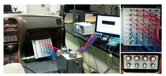
Figure 8.
Vehicle diagnostics simulator: HYUNDAI SIRIUS-II engine, NI 9221 data acquisition device, and eight sensor voltage controllers.
In this study, we artificially generated the fault that stops the engine by increasing an amount of air in the intake manifold. It was conducted with following steps:
- Step 1. Turn on the engine
- Step 2. Control the amount of manifold air flow
- Step 3. An engine knocking occurs
The data in no-fault state was collected during Step 1 and Step 2, while the data in the fault state was collected in Step 3.
The sensor signals show high aVar, DI, DF, and CI. By FP1, we could detect 46 engine faults, while all of the 46 faults were identified by FP2.
3.3. Automotive Buzz, Squeak, and Rattle (BSR) Noise Monitoring Data
The BSR noise monitoring data, as shown in Figure 6c, were collected from the automotive BSR monitoring system, as shown in Figure 9. BSR noises are induced by a friction between automotive subcomponents. The system was developed to detect a defective car door trim during an assembly process that has a potential to generate BSR noises. The developed in-process BSR noise detection system consists of a sensor array of nine microphones, four parabolic microphones, a pneumatic pusher controlled by a gantry robot, a data acquisition system, NI cDAQ-9178TM (National Instruments, Austin, TX, USA), and a noise detection software that we developed.
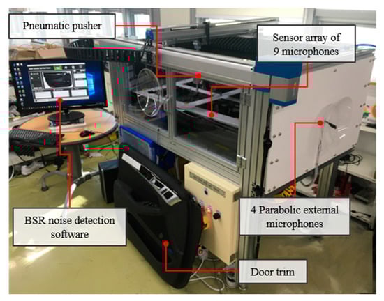
Figure 9.
Automotive BSR noise monitoring system: a sensor array of nine microphones, four parabolic microphones, a pneumatic pusher controlled by a gantry robot, and NI cDAQ-9178 TM data acquisition device.
A car door trim was slowly pressed down by a pneumatic pusher with a pressure of 10 kgf/cm2. We then monitor the acoustic signals measured right above the door trim by a microphone array in order to identify BSR noises. We determined the state of a door trim whether it generated abnormal sounds when pressed by a pneumatic pusher.
The sensor signals show low aVar and CI but high DI and DF. By FP1, we could detect 80% of the fault states, while all the fault states were identified by FP2.
3.4. Marine Diesel Engine Data
Marine diesel engine data, shown in Figure 6e, were collected from a marine diesel engine (Type 9H32/30, Hyundai Heavy Industries, Ulsan, Korea). We selected six major sensors in the modularized feed system among the 482 sensors installed in the engine. We defined the abnormal combustion as the fault state of the engine. It has usually occurred when a cylinder’s temperature exceeds a predefined control limit. The sensor data shows low values for aVar, DI, DF, and CI. By FP1, we could detect 93% of the fault states, while all of the fault states were identified by FP2.
4. Concluding Remarks
The four different datasets were analyzed with two different discretization-based fault pattern extraction methods. The results demonstrated that the fault pattern extraction performances were closely related with the KCIs. The performance of FP2 decreased as the DF and CI increased; in particular, the laser welding data showed the lowest performance (40%) together with the highest DF and CI values. When the DF is high, FP2 cannot generate enough fault patterns due to low event code variation between the no-fault and the fault states. The performance of FP2 also decreases as DI increases.
Based on these empirical studies, we can provide a guideline for selecting an appropriate label definition method in accordance with the KCIs of the given multivariate time series data. By definition, if the difference between no-fault and fault states is more distinct in the frequency domain, then the CI value will be relatively low. We observed that the frequency variation based discretization method produced a better result when the CI is low.
In summary, we have proposed a new fault pattern extraction method using frequency variation-based discretization. For fault pattern extraction, first, the time series of a sensor signal is discretized to create a set of labels representing the dominant frequency of each time segment. Second, the pattern is generated by converting series of labels into a set of event codes. Third, the fault patterns are determined as the patterns that only occur in a fault state of a system.
In addition, we have investigated a relation between the KCIs and the performance of fault pattern extraction using both amplitude and frequency variation, providing a guideline for selecting appropriate label definitions. The results show that the CI, the aggregated index of the DF and the DI, can be used as a good reference for selecting an appropriate label definition method. For example, the fault pattern performance of FP2 decreased as DF and CI increased. In contrast, aVar was only weakly related to the FP2 performance. Furthermore, the FP1 performance decreased as the DI increased, whereas CI decreased. The experimental result confirmed that the frequency variation based discretization method produced better result when the CI is low. Since the fault pattern performance is also closely related to the discretization parameters, and therefore, further empirical study is necessary.
Acknowledgments
This research was supported by Basic Science Research Program through the National Research Foundation of Korea (NRF) funded by the Ministry of Education (2017R1D1A1B04036509).
Author Contributions
Woonsang Baek and Sujeong Baek conceived and designed, performed, and analyzed the experiments and wrote the paper under the guidance of Duck Young Kim.
Conflicts of Interest
The authors declare no conflict of interest.
References
- Venkatasubramanian, V.; Rengaswamy, R. A review of process fault detection and diagnosis: Part iii: Process history based methods. Comput. Chem. Eng. 2003, 27, 327–346. [Google Scholar] [CrossRef]
- Isermann, R. Model-based fault-detection and diagnosis–status and applications. Ann. Rev. Control 2005, 29, 71–85. [Google Scholar] [CrossRef]
- Hellerstein, J.M.; Koutsoupias, E.; Papadimitriou, C.H. On the analysis of indexing schemes. In Proceedings of the Sixteenth ACM SIGACT-SIGMOD-SIGART Symposium on Principles of Database Systems, Tucson, AZ, USA, 11–15 May 1997. [Google Scholar]
- Nguyen, S.H.; Nguyen, H.S. Pattern extraction from data. Fundam. Inform. 1998, 34, 129–144. [Google Scholar]
- Lin, J.; Keogh, E.; Wei, L.; Lonardi, S. Experiencing sax: A novel symbolic representation of time series. Data Min. Knowl. Discov. 2007, 15, 107–144. [Google Scholar] [CrossRef]
- Pensa, R.G.; Leschi, C.; Besson, J.; Boulicaut, J.-F. Assessment of discretization techniques for relevant pattern discovery from gene expression data. In Proceedings of the Fourth International Conference on Data Mining in Bioinformatics, Copenhagen, Denmark, 28–29 April 2018. [Google Scholar]
- Dash, R.; Paramguru, R.L.; Dash, R. Comparative analysis of supervised and unsupervised discretization techniques. Int. J. Adv. Sci. Technol. 2011, 2, 29–37. [Google Scholar]
- Liu, H.; Hussain, F.; Tan, C.L.; Dash, M. Discretization: An enabling technique. Data Min. Knowl. Discov. 2002, 6, 393–423. [Google Scholar] [CrossRef]
- Dougherty, J.; Kohavi, R.; Sahami, M. Supervised and unsupervised discretization of continuous features. In Proceedings of the Twelfth International Conference on Machine Learning, Tahoe City, CA, USA, 9–12 July 1995. [Google Scholar]
- Wong, A.K.; Chiu, D.K. Synthesizing statistical knowledge from incomplete mixed-mode data. IEEE Trans. Pattern Anal. Mach. Intell. 1987, PAMI-9, 796–805. [Google Scholar] [CrossRef]
- Gupta, A.; Mehrotra, K.G.; Mohan, C. A clustering-based discretization for supervised learning. Stat. Probab. Lett. 2010, 80, 816–824. [Google Scholar] [CrossRef]
- Halim, E.B.; Choudhury, M.A.A.S.; Shah, S.L.; Zuo, M.J. Time domain averaging across all scales: A novel method for detection of gearbox faults. Mech. Syst. Signal Proc. 2008, 22, 261–278. [Google Scholar] [CrossRef]
- Huang, N.; Qi, J.; Li, F.; Yang, D.; Cai, G.; Huang, G.; Zheng, J.; Li, Z. Short-circuit fault detection and classification using empirical wavelet transform and local energy for electric transmission line. Sensors 2017, 17, 2133. [Google Scholar] [CrossRef] [PubMed]
- Zarei, J.; Poshtan, J. Bearing fault detection using wavelet packet transform of induction motor stator current. Tribol. Int. 2007, 40, 763–769. [Google Scholar] [CrossRef]
- Wang, H.; Li, R.; Tang, G.; Yuan, H.; Zhao, Q.; Cao, X. A compound fault diagnosis for rolling bearings method based on blind source separation and ensemble empirical mode decomposition. PLoS ONE 2014, 9, e109166. [Google Scholar] [CrossRef] [PubMed]
- Lu, C.; Wang, Y.; Ragulskis, M.; Cheng, Y. Fault diagnosis for rotating machinery: A method based on image processing. PLoS ONE 2016, 11, e0164111. [Google Scholar] [CrossRef] [PubMed]
- Chen, X.; Feng, F.; Zhang, B. Weak fault feature extraction of rolling bearings based on an improved kurtogram. Sensors 2016, 16, 1482. [Google Scholar] [CrossRef] [PubMed]
- Lee, J.J.; Lee, S.M.; Kim, I.Y.; Min, H.K.; Hong, S.H. Comparison between short time fourier and wavelet transform for feature extraction of heart sound. In Proceedings of the IEEE Region 10 Conference TENCON 99, Cheju Island, Korea, 15–17 September 1999. [Google Scholar]
- Yang, J.; Hamelin, F.; Sauter, D. Fault detection observer design using time and frequency domain specifications. IFAC Proc. Vol. 2014, 47, 8564–8569. [Google Scholar] [CrossRef]
- Patton, R.; Chen, J. Observer-based fault detection and isolation: Robustness and applications. Control Eng. Pract. 1997, 5, 671–682. [Google Scholar] [CrossRef]
- Chibani, A.; Chadli, M.; Shi, P.; Braiek, N.B. Fuzzy fault detection filter design for t–s fuzzy systems in the finite-frequency domain. IEEE Trans. Fuzzy Syst. 2017, 25, 1051–1061. [Google Scholar] [CrossRef]
- Li, L.; Chadli, M.; Ding, S.X.; Qiu, J.; Yang, Y. Diagnostic observer design for ts fuzzy systems: Application to real-time weighted fault detection approach. IEEE Trans. Fuzzy Syst. 2017. [Google Scholar] [CrossRef]
- Chibani, A.; Chadli, M.; Braiek, N.B. A finite frequency approach to h∞ filtering for T–S fuzzy systems with unknown inputs. Asian J. Control 2016, 18, 1608–1618. [Google Scholar] [CrossRef]
- Dai, X.; Gao, Z. From model, signal to knowledge: A data-driven perspective of fault detection and diagnosis. IEEE Trans. Ind. Inform. 2013, 9, 2226–2238. [Google Scholar] [CrossRef]
- Naderi, E.; Khorasani, K. Data-driven fault detection, isolation and estimation of aircraft gas turbine engine actuator and sensors. In Proceedings of the 2017 IEEE 30th Canadian Conference on Electrical and Computer Engineering (CCECE), Windsor, ON, Canada, 30 April–3 May 2017. [Google Scholar]
- McInerny, S.A.; Dai, Y. Basic vibration signal processing for bearing fault detection. IEEE Trans. Educ. 2003, 46, 149–156. [Google Scholar] [CrossRef]
- Byington, C.S.; Watson, M.; Edwards, D. Data-driven neural network methodology to remaining life predictions for aircraft actuator components. In Proceedings of the 2004 IEEE Proceedings on Aerospace Conference, Big Sky, MT, USA, 6–13 March 2004. [Google Scholar]
- Sejdić, E.; Jiang, J. Pattern Recognition Techniques, Technology and Applications; InTech: Vienna, Austria, 2008. [Google Scholar]
- Baek, S.; Kim, D.Y. Empirical sensitivity analysis of discretization parameters for fault pattern extraction from multivariate time series data. IEEE Trans. Cybern. 2017, 47, 1198–1209. [Google Scholar] [CrossRef] [PubMed]
- Peng, Z.K.; Chu, F.L. Application of the wavelet transform in machine condition monitoring and fault diagnostics: A review with bibliography. Mech. Syst. Signal Proc. 2004, 18, 199–221. [Google Scholar] [CrossRef]
- Fu, T.-C. A review on time series data mining. Eng. Appl. Artif. Intell. 2011, 24, 164–181. [Google Scholar] [CrossRef]
© 2018 by the authors. Licensee MDPI, Basel, Switzerland. This article is an open access article distributed under the terms and conditions of the Creative Commons Attribution (CC BY) license (http://creativecommons.org/licenses/by/4.0/).