Measurement of Walking Ground Reactions in Real-Life Environments: A Systematic Review of Techniques and Technologies


Abstract
1. Introduction
- -
- Quantification of the spatiotemporal gait fluctuations over time or due to environmental, behavioural or contextual factors are essential in many applications such as understanding the motor control of gait, quantifying pathologic and age-related alterations in the locomotor control system, and augmenting objective measurement of mobility and functional status [6]. However, It is shown that measuring a limited number of strides in the gait laboratory may not represent natural cycle-by-cycle gait variations [7].
- -
- Recent studies showed that subjects may modify their gait inside laboratory environment and may mask or exaggerate their problem during the test [8].
- -
- The standard two-forceplates setup used in biomechanics laboratories makes it possible to measure ground reactions for only one step and enforces a limited area for foot placement, which can alter the natural gait [9,10,11,12,13,14,15]. The instrumented treadmills, on the other hand, can record continuous walking/running of a test subject [10,12]. However, they can only record the ground reactions while subject is moving in a straight line with a constant speed [16].
- -
- The standard gait laboratory equipment (optical motion capture, force plates and instrumented treadmills) are very expensive and cumbersome and require expertise to operate [16]. These factors restrict their availability to a limited number of well-equipped gait laboratories.
- -
- Long-term measurement of gait in real-life environment is essential in many applications including quantification of disease progression [17], monitoring the effects of treatment [18], and monitoring alteration of performance biomarkers in professional sports [19,20]. Realistic monitoring of the dynamic gait variations can signify disease severity and medication utility, and can be used to document quantitatively improvements in response to therapeutic interventions, significantly more effective than what can be learned based on the average, typical stride measured in a laboratory [6].
- -
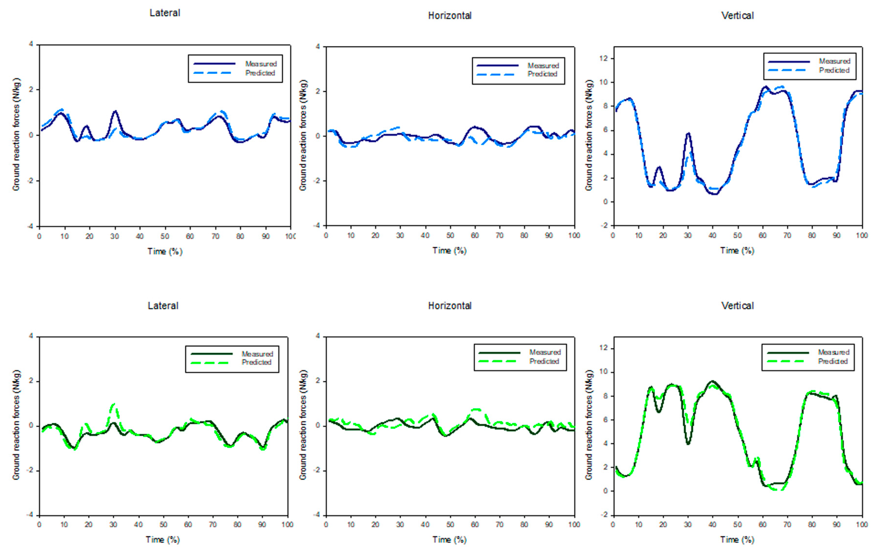
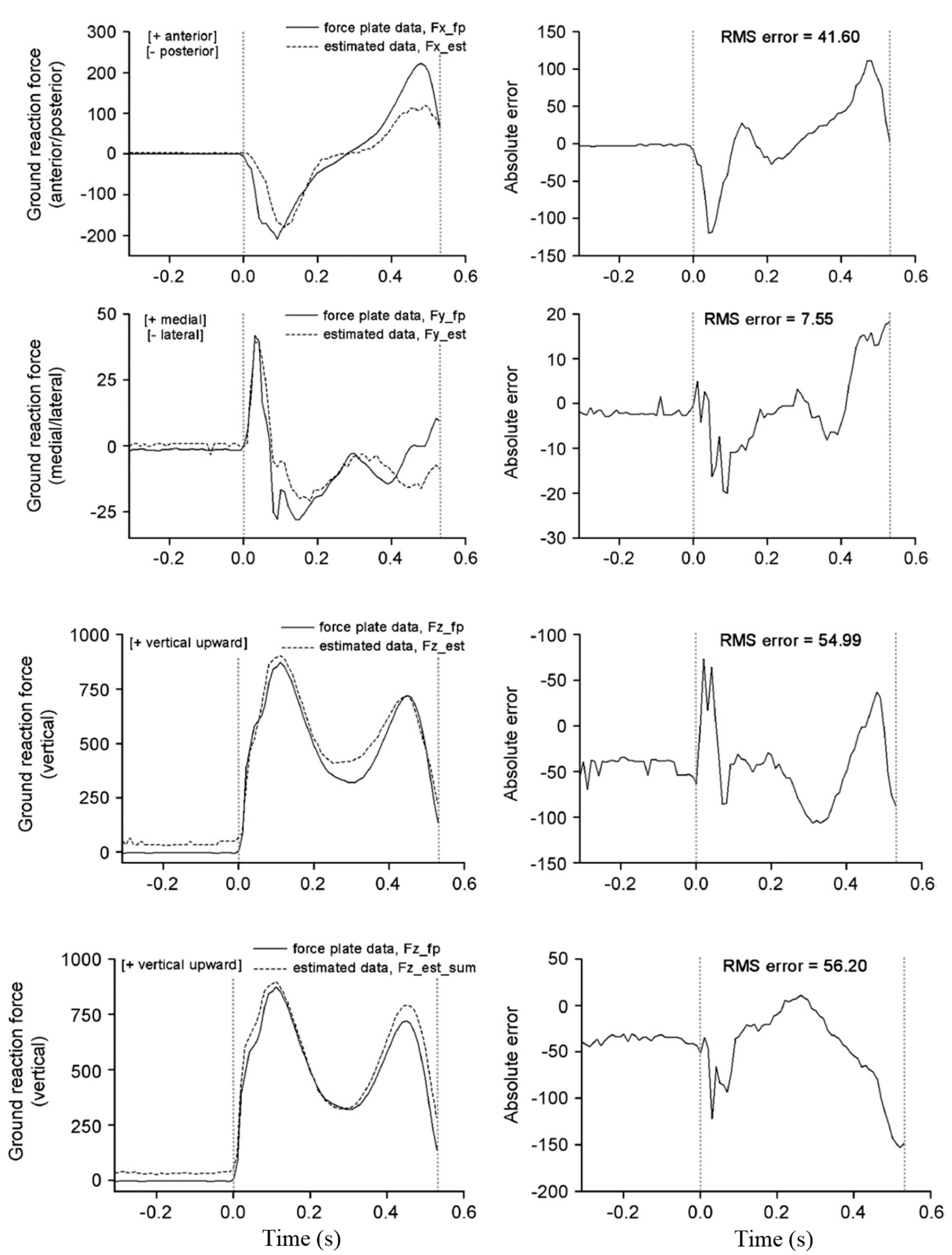
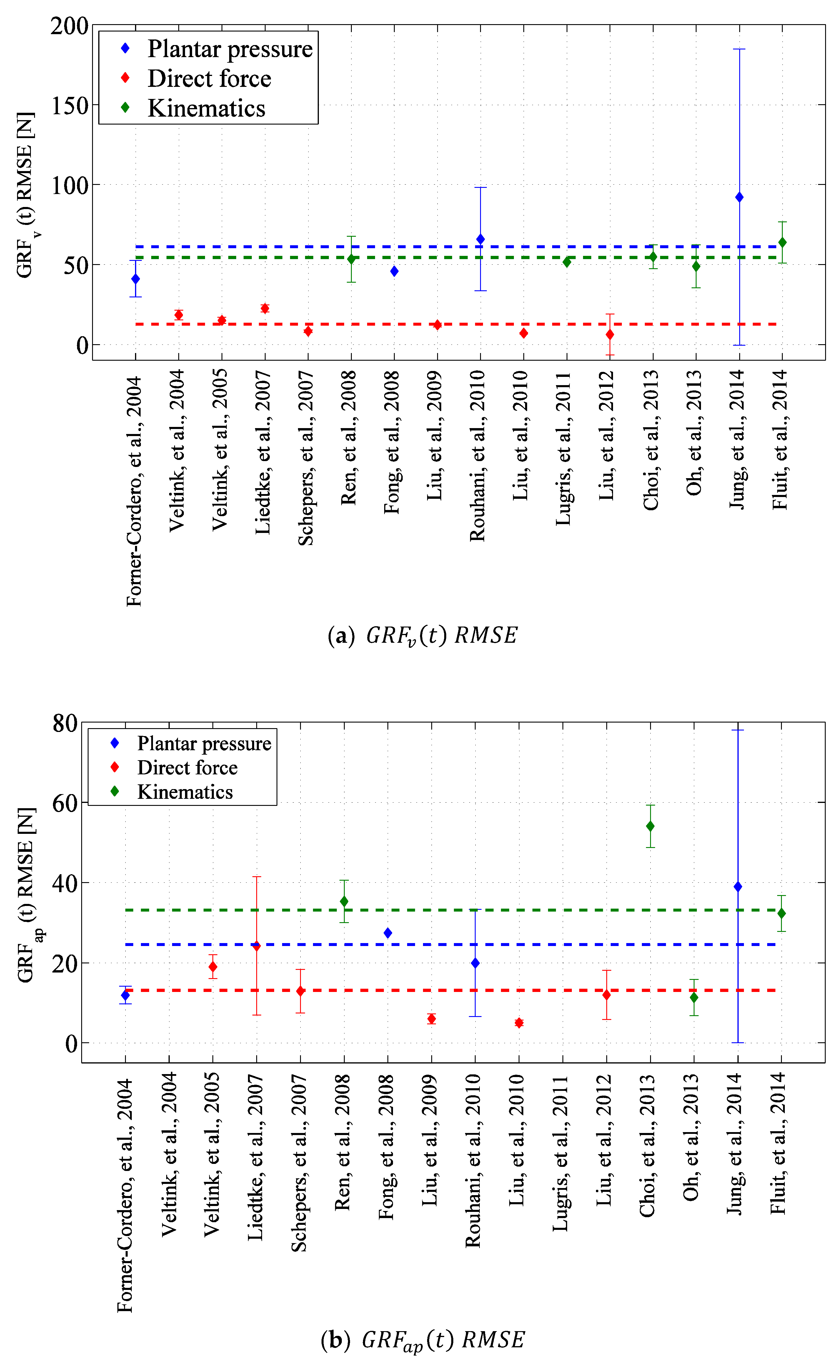
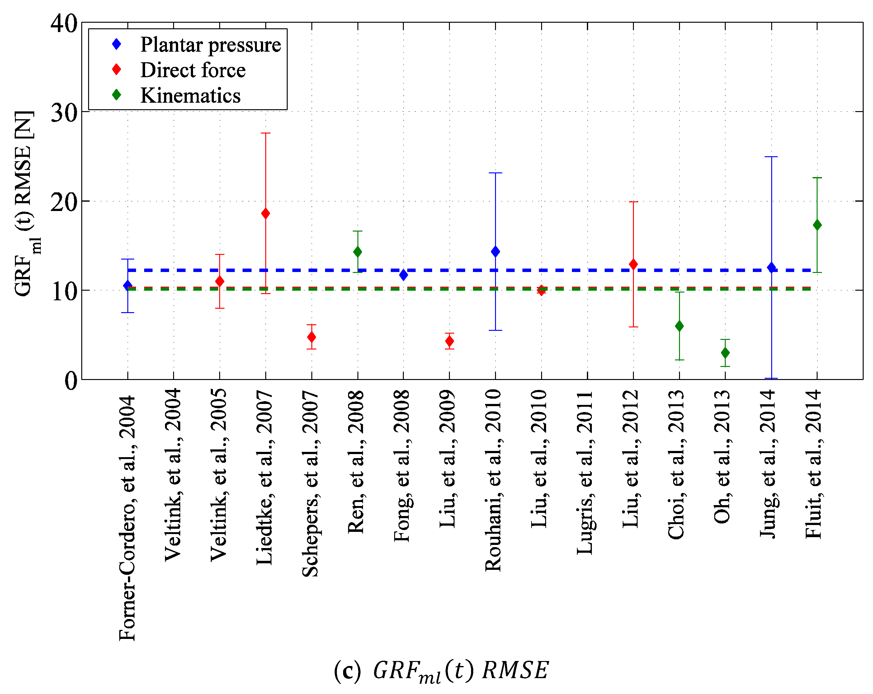
- Methods based on measured kinematic data use a human body dynamic model to estimate , and/or signals from acceleration of different body segments. This category of techniques can potentially use the inexpensive and durable wearable Inertial Measurement Units (IMUs) for measuring body kinematics and therefore are potentially practical. Although these methods are prone to IMU errors in orientation measurement and are sensitive to the characteristics of the body dynamic model, they have shown competitive accuracy of 54 N, 33 N and 10 N root-mean-square-error (RMSE) (assuming an average subject weight of 750 N) for estimating and , respectively.
- -
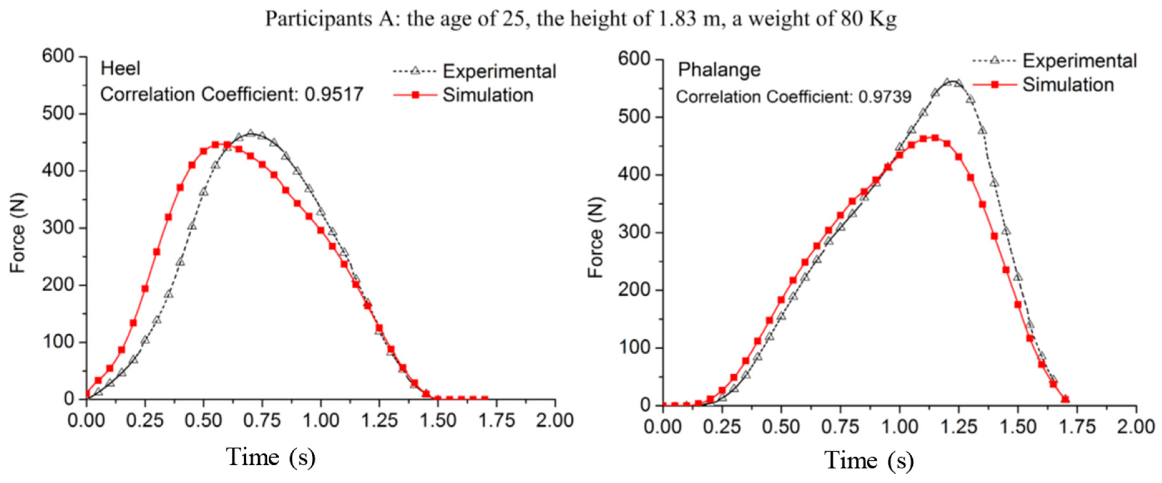
- Methods based on measured plantar pressure use a matrix of insole pressure sensors to measure plantar pressure of each foot perpendicular to the contact surface. A computational method is usually used to estimate tri-axial and plantar signals. Although current pressure insole sensors show limited durability and high sensitivity to their boundary condition in the shoe, this category of method have shown to achieve competitive average accuracy of 61 N, 25 N and 12 N RMSE for estimating and , respectively.
- -
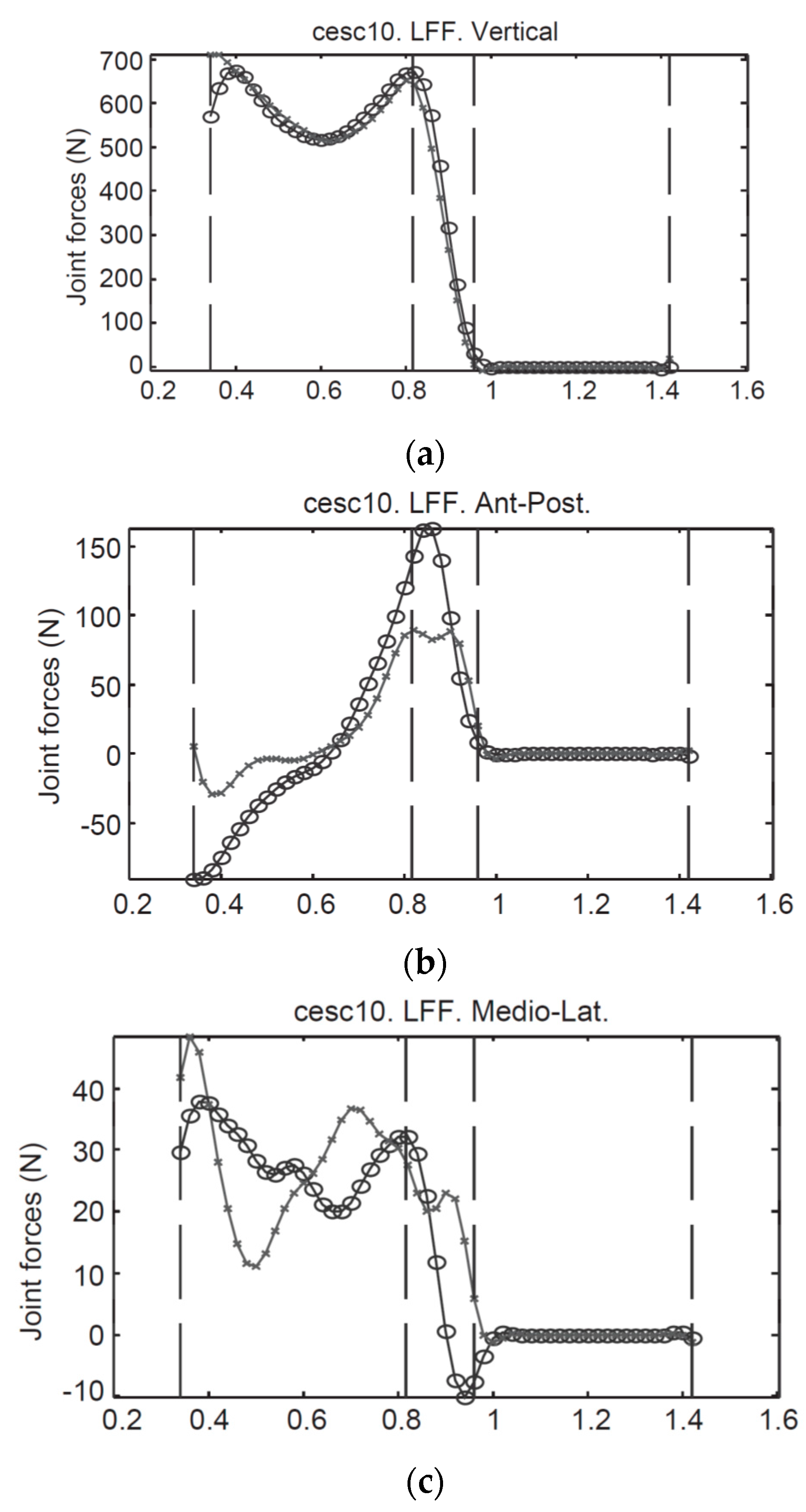
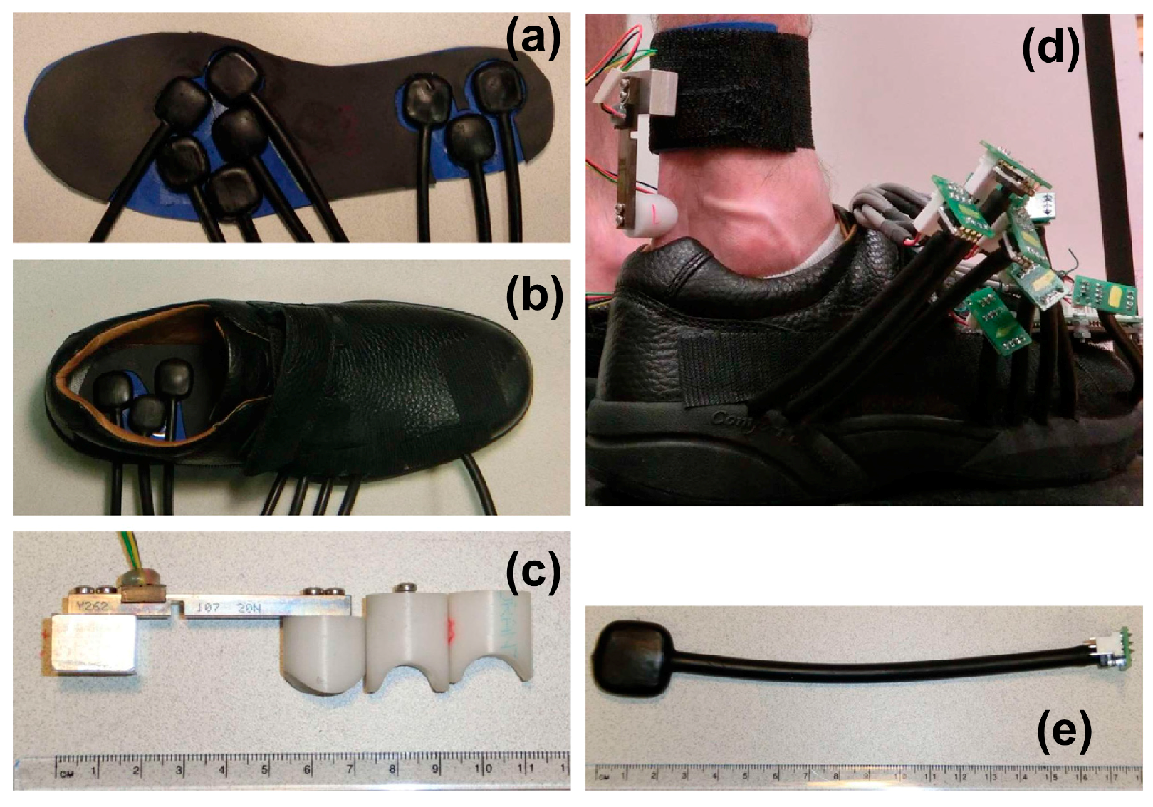
- Methods based on force measurement directly measure tri-axial and signals under each foot using a pair of shoes instrumented with tri-axial force sensors and IMUs. Although the cumbersome electromechanical form factor of these systems can affect the natural gait and reduce its practicality, this class of techniques is shown to achieve the highest average accuracy of 13 N, 13 N and 10 N RMSE for estimating and , respectively.
2. Data Analysis
3. Methods Based on Measured Kinematic Data
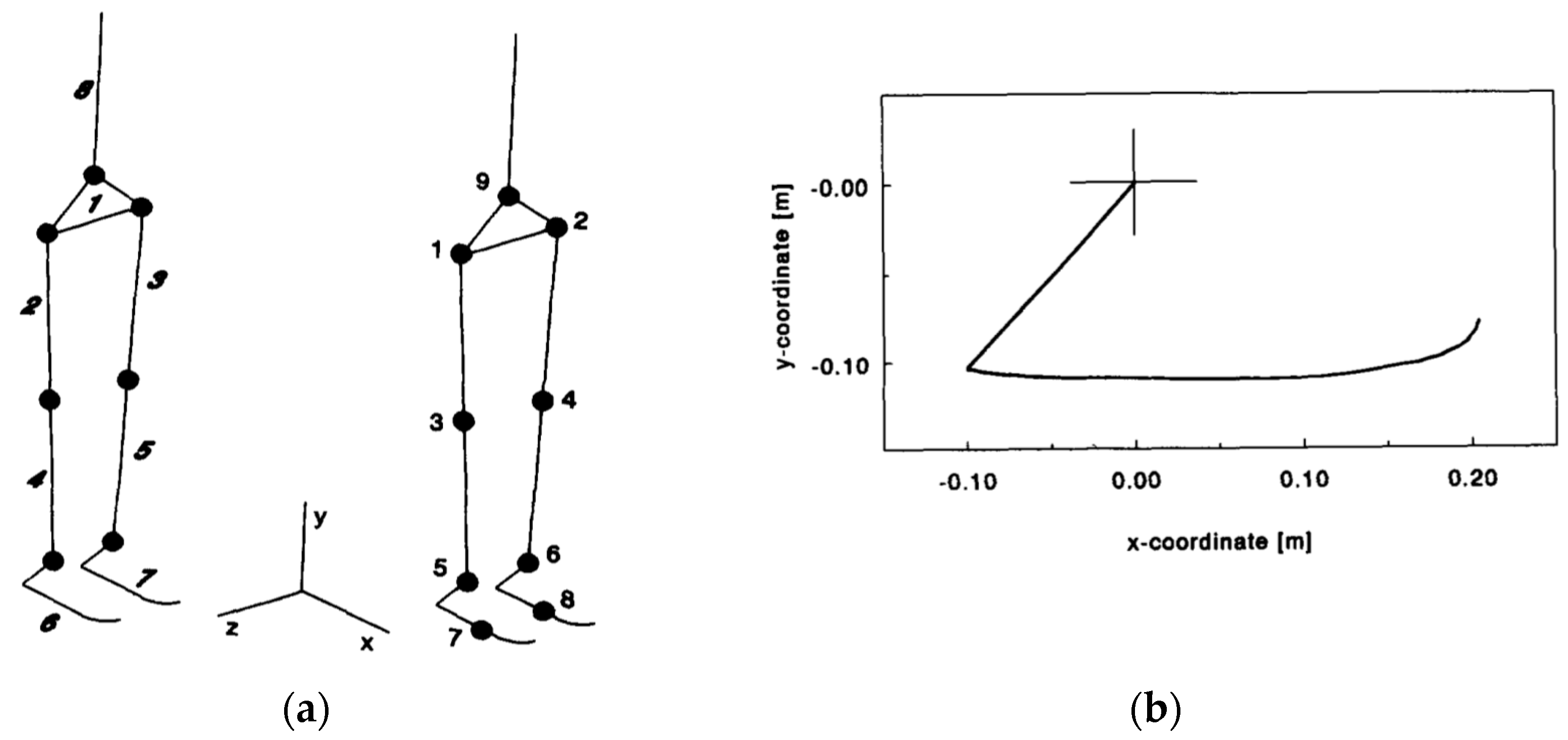
3.1. Double-Support Indeterminacy
- -
- The joints are frictionless pin-joints;
- -
- The body segments are assumed to be rigid, with their mass concentrated at their centres of mass;
- -
- The co-contraction of agonist and antagonist muscles are neglected;
- -
- The air friction is assumed to be negligible.
3.2. Methods
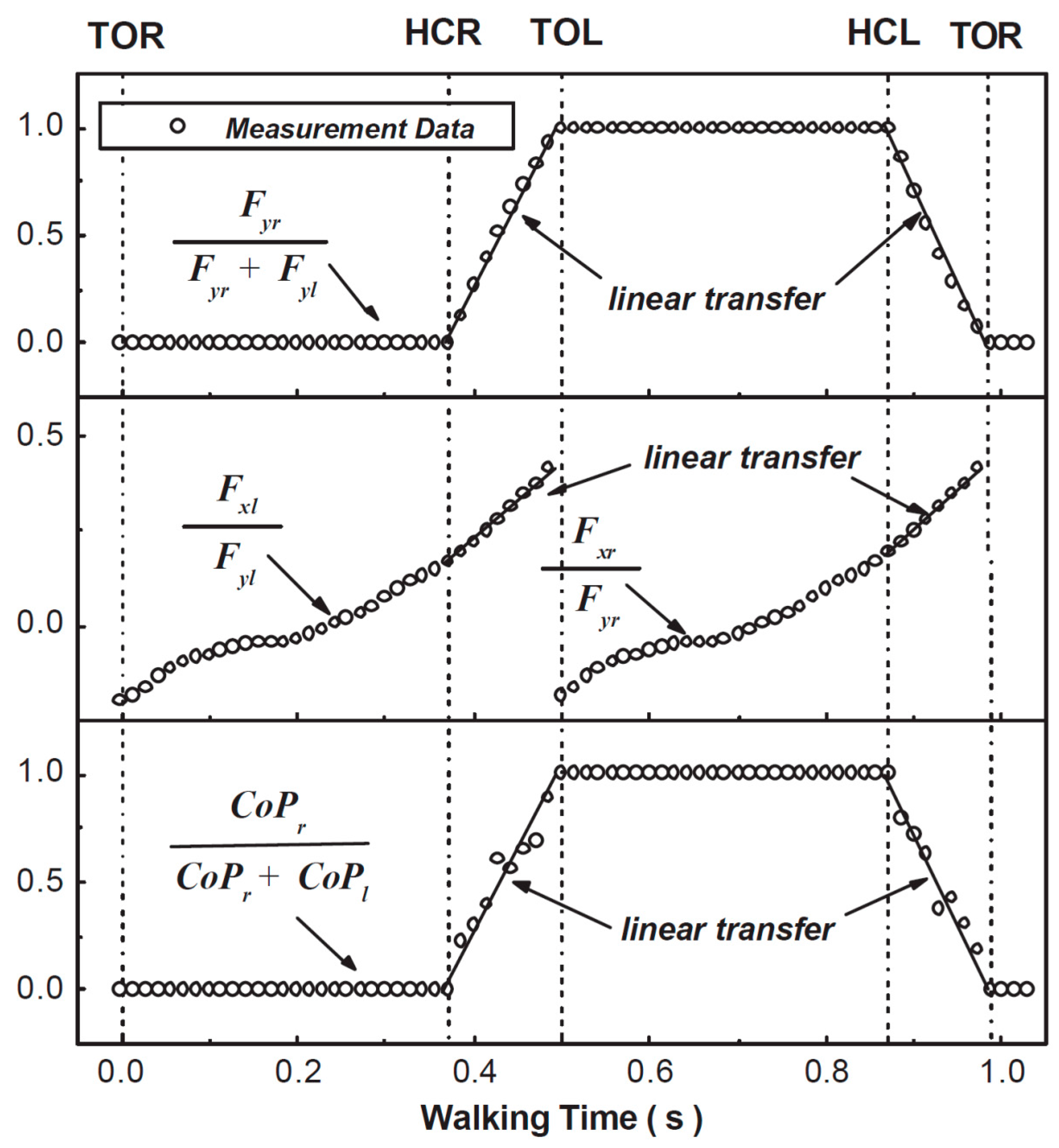
- -
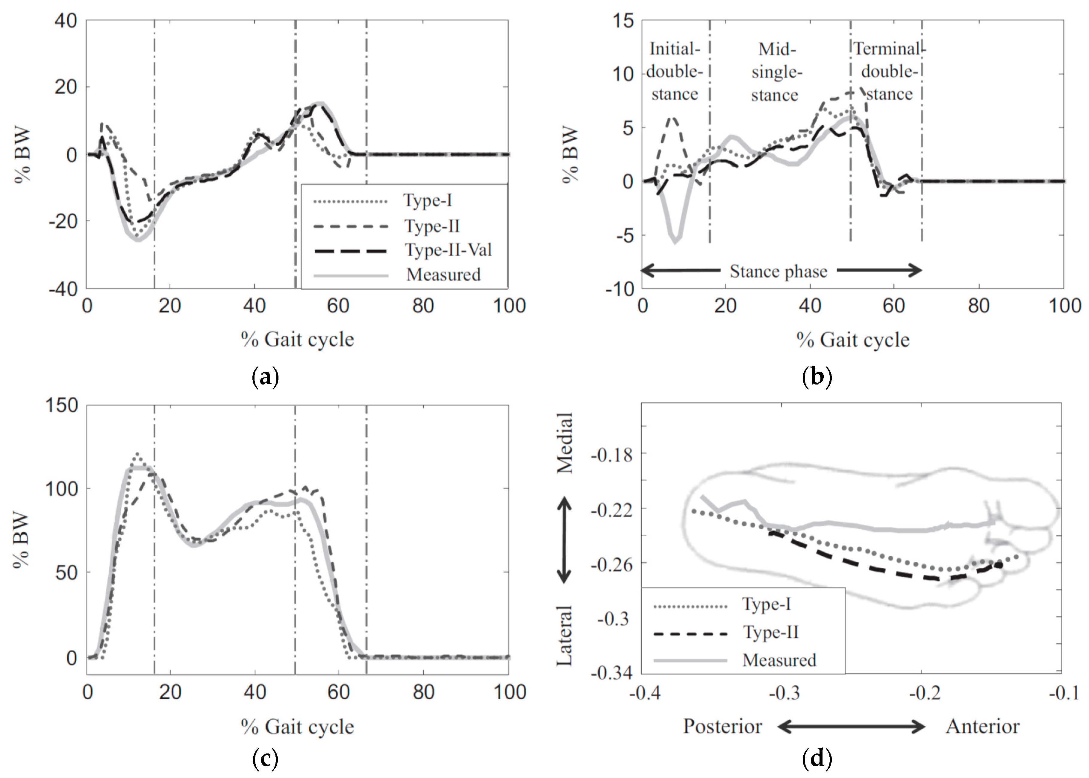
- The ratio of the on the heel-strike foot to the total varies linearly during the DSP (Figure 3, top).
- -
- The ratio of the to the on the toe-off foot varies linearly during the DSP (Figure 3, middle).
- -
- The ratio of for the heel-strike foot to the sum of the for both feet varies linearly during the DSP (Figure 3, bottom).
- -
- and signals of the trailing foot reduce smoothly to zero during the DSP.
- -
- The ratios of signals to their values at contralateral heel strike (i.e., the non-dimensional ground reactions) can be expressed as functions of DSP duration (termed transition functions).
3.3. Comparison of the Methods
4. Methods Based on Measured Plantar Pressure
4.1. Methods
4.2. Comparison of Methods
5. Methods Based on Tri-Axial Force Measurement
5.1. Methods
5.2. Comparison of Methods
6. Discussion
- -
- Kinematics-based methods: (1) these methods rely on a dynamic human model to estimate , and signals. It has been shown that the accuracy of the estimated signals is very sensitive to the characteristics of the human model such as foot [106] and knee joint [107] models. This can be a source of significant uncertainty in the accuracy of the model outputs; (2) errors in measured kinematic data, particularly errors in the measured orientations in the case of using wearable IMUs [108]; (3) the simplifying assumptions used in body dynamic model and the inverse dynamics analysis, such as solid body segments and frictionless joints; (4) the inaccuracies in anthropometric data, particularly the size, density and weight of body segments, the location of joint centres and the location of centre of mass of each body segment; (5) soft tissue artefacts (STA) [109,110]; and (6) inherent computational errors of the methods proposed to solve the indeterminacy problem of the closed-kinematic chain during DSP.
- -
- Methods based on measurement of Plantar pressure: (1) the low accuracy and rapid deterioration (resulting in time varying calibration) of the pressure sensors; (2) high sensitivity of the insole pressure sensors to their boundary conditions in the shoe [111]; and (3) the errors associated with the estimation of tri-axial signals from uniaxial plantar pressure data.
- -
- Methods based on direct measurement of : (1) errors associated with estimating forces and moments in the coordinate systems of body segments and joints, because of uncertainties in relative positions and deformation of segments, especially of the foot [91]; (2) errors associated with IMU orientation measurement as instrumented shoes use IMUs to measure the orientation of each sensor with respect to the global/body coordinate system.
- -
- Versatility and Robustness: many of the discussed methods are only validated for a particular movement [36,37] or methodologies are developed based on a limited dataset [38,39] that may not be applicable for movements other than those present in the dataset. To be able to use the proposed methodologies in real-life setting, it is important for the method to be robust and versatile enough to handle different movements and ambulation abnormalities. Future proposed methods could try to analyse the performance of the method for different ambulatory regimes, pathological gaits and physical environment conditions such as slopes, slippery surfaces, etc., and to provide experimental validation for such scenarios. For instance, knowing that real-life meausrement entails monitoring not only walking but several different activates such as sitting, turning, running, etc., combining a set of activity-specific estimation methods with and activity recognition method to link the type of activity with corresponding estimation method could be a possible direction for tackling this problem.
- -
- Training requirement: Due to the inter- and intra- subject variability of human gait, many of the estimation methods, including the ones based on Artificial Neural Networks [26,48], rely on training data for calibration. However, such training data might not be available. Therefore, it is desirable for the methodologies not to require training data or to provide a generic form that works with reasonable accuracy for the cases where training data is not available. Considering the potential benefits of personalizing the parameters of estimation methods, an interesting avenue for the future research could be to develop methodologies that autonomously self-train and personalize their parameters using only the available sensors of the system.
- -
- System design: Minimizing the size and weight of the sensors and data acquisition systems, reducing their power demand and increasing their battery life, particularly through methods such as energy harvesting from ambulation [112] are fundamental to the application of these systems for long-term monitoring.
7. Conclusions
Acknowledgments
Conflicts of Interest
Nomenclature
| Linear acceleration of the centre of mass of body segment ‘i’ | |
| Angular acceleration around the centre of mass of the body segment ‘i’ | |
| ADL | Activities of daily living |
| ANN | Artificial neural network |
| BMI | Body mass index |
| CoM | Centre of mass |
| CoP | Centre of plantar pressure |
| DSP | Double-support phase |
| DoF | Degree of Freedom |
| FCM | Foot-ground contact model |
| GRF | Ground reaction force |
| Ground reaction force in the vertical direction | |
| Ground reaction force in the anterior-posterior direction | |
| Ground reaction force in the medial-lateral direction | |
| GRM | Ground reaction moment |
| Second moment of inertia of the body segment ‘i’ | |
| ID | Inverse dynamics |
| IMU | Inertial measurement unit |
| and | Empirical constants |
| Mass of the body segment ‘i’ | |
| Number of (solid) body segments | |
| NRMSE | Normalised root mean square error |
| PCI-MI | Principal component analysis—mutual information |
| R | Cross-correlation coefficient |
| Moment arm pertinent to the body segment ‘i’ | |
| RMSE | Root mean square error |
| SLR | Stepwise linear regression |
| SSP | Single-support phase |
| Half of the double-support duration | |
| WNN | Wavelet neural network |
References
- Vaughan, C.L.; Davis, B.L.; Christopher, L.; O’Connor, J.C. Dynamics of Human Gait; Human Kinetics Publishers: Champaign, IL, USA, 1992. [Google Scholar]
- Levine, D.F.; Richards, J.; Whittle, M. Whittle’s Gait Analysis; Elsevier Health Sciences: Amsterdam, The Netherlands, 2012; ISBN 978-070204265. [Google Scholar]
- Winter, D.A. Human balance and posture control during standing and walking. Gait Posture 1995, 3, 193. [Google Scholar] [CrossRef]
- Aminian, K.; Najafi, B. Capturing human motion using body-fixed sensors: Outdoor measurement and clinical applications. Comput. Anim. Virtual Worlds 2004, 15, 79–94. [Google Scholar] [CrossRef]
- Najafi, B.; Helbostad, J.L.; Moe-Nilssen, R.; Zijlstra, W.; Aminian, K. Does walking strategy in older people change as a function of walking distance? Gait Posture 2009, 29, 261–266. [Google Scholar] [CrossRef] [PubMed]
- Hausdorff, J.M. Gait dynamics, fractals and falls: Finding meaning in the stride-to-stride fluctuations of human walking. Hum. Mov. Sci. 2007, 26, 555–589. [Google Scholar] [CrossRef] [PubMed]
- Veltink, H.; Liedtke, C.; Droog, E. Ambulatory measurement of ground reaction forces. In Proceedings of the IEEE International Conference on Systems, Man and Cybernetics, Hague, The Netherlands, 10–13 October 2004. [Google Scholar]
- Najafi, B.; Khan, T.; Wrobel, J. Laboratory in a Box: Wearable Sensors and Its Advantages for Gait Analysis. In Proceedings of the 33rd Annual International Conference of the IEEE EMBS, Boston, MA, USA, 30 August–3 September 2011. [Google Scholar] [CrossRef]
- Hausdorff, J.M.; Cudkowicz, M.E.; Firtion, R.; Wei, J.Y.; Goldberger, A.L. Gait variability and basal ganglia disorders: Stride-to-stride variations of gait cycle timing in Parkinson’s disease and Huntington’s disease. Mov. Disord. 1998, 13, 428–437. [Google Scholar] [CrossRef] [PubMed]
- Belli, A.; Bui, P.; Berger, A.; Geyssant, A.; Lacour, J.R. A treadmill ergometer for three-dimensional ground reaction forces measurement during walking. J. Biomech. 2001, 34, 105–112. [Google Scholar] [CrossRef]
- Rabuffetti, M.; Frigo, C. Ground reaction: Intrinsic and extrinsic variability assessment and related method for artefact treatment. J. Biomech. 2001, 34, 363–370. [Google Scholar] [CrossRef]
- Verkerke, G.J.; Hof, A.L.; Zijlstra, W.; Ament, W.; Rakhorst, G. Determining the center of pressure during walking and running using an instrumented treadmill. J. Biomech. 2005, 38, 1881–1885. [Google Scholar] [CrossRef] [PubMed]
- Segal, A.D.; Orendurff, M.S.; Czerniecki, J.M.; Shofer, J.B.; Klute, G.K. Local dynamic stability in turning and straight-line gait. J. Biomech. 2008, 41, 1486–1493. [Google Scholar] [CrossRef] [PubMed]
- Pandy, M.G.; Lin, Y.C.; Kim, H.J. Muscle coordination of medial-lateral balance in normal walking. J. Biomech. 2010, 43, 2055–2064. [Google Scholar] [CrossRef] [PubMed]
- Chen, Y.C.; Lou, S.Z.; Huang, C.Y.; Su, F.C. Effects of foot orthoses on gait patterns of flat feet patients. J. Clin. Biomech. 2010, 25, 265–270. [Google Scholar] [CrossRef] [PubMed]
- Tao, W.; Liu, T.; Zheng, R.; Feng, H. Gait Analysis Using Wearable Sensors. Sensors 2012, 12, 2255–2283. [Google Scholar] [CrossRef] [PubMed]
- Del Din, S.; Godfrey, A.; Rochester, L. Validation of an accelerometer to quantify a comprehensive battery of gait characteristics in healthy older adults and Parkinson’s disease: Toward clinical and at home use. IEEE J. Biomed. Health Inform. 2015, 2194, 1–10. [Google Scholar] [CrossRef] [PubMed]
- Bussmann, J.B.J.; Veltink, P.H.; Koelma, F.; Lummel, R.C.; Stam, H.J. Ambulatory monitoring of mobility-related activities: The initial phase of the development of an activity monitor. Eur. J. Phys. Rehabil. Med. 1995, 5, 2–7. [Google Scholar]
- Watanabe, K.; Hokari, M. Kinematical analysis and measurement of sports form. IEEE Trans. Syst. Man Cybern. Part A 2006, 36, 549–557. [Google Scholar] [CrossRef]
- Kwon, D.Y.; Gross, M. Combining body sensors and visual sensors for motion training. In Proceedings of the 2005 ACM SIGCHI International Conference on Advances in Computer Entertainment Technology, Valencia, Spain, 15–17 June 2005; pp. 94–101. [Google Scholar]
- Liberati, A.; Altman, D.G.; Tetzlaff, J.; Mulrow, C.; Gøtzsche, P.C.; Ioannidis, J.P.; Clarke, M.; Devereaux, P.J.; Kleijnen, J.; Moher, D. The PRISMA Statement for Reporting Systematic Reviews and Meta-Analyses of Studies that Evaluate Health Care Interventions: Explanation and Elaboration. PLoS Med. 2009, 6, e1000100. [Google Scholar] [CrossRef] [PubMed]
- Winter, D.A. The Biomechanics and Motor Control of Human Movement, 2nd ed.; Wiley: New York, NY, USA, 1990. [Google Scholar]
- Luinge, H.J.; Veltink, P.H. Measuring orientation of human body segments using miniature gyroscopes and accelerometers. Med. Biol. Eng. Comput. 2005, 43, 273–282. [Google Scholar] [CrossRef] [PubMed]
- Winter, D.A. The Biomechanics and Motor Control of Human Gait: Normal, Elderly and Pathological; University of Waterloo Press: Waterloo, ON, Canada, 1991. [Google Scholar]
- Zatsiorsky, V.M. Kinematics of Human Motion; Human Kinetics: Champaign, IL, USA, 1998. [Google Scholar]
- Oh, S.E.; Choi, A.; Mun, J.H. Prediction of ground reaction forces during gait based on kinematics and a neural network model. J. Biomech. 2013, 46, 2372–2380. [Google Scholar] [CrossRef] [PubMed]
- Quanbury, A.O.; Winter, D.A. Calculation of floor reaction forces from kinematic data during single, support phase of human gait. In Proceedings of the V Canadian Medical and Biological Engineering Conference, Montreal, QC, Canada, 1974. [Google Scholar]
- Robertson, D.G.E.; Winter, D.A. Estimation of Ground Reaction Forces from Kinematics and Body Segment Parameters; Canadian Association of Sport Sciences: Vancouver, BC, Canada, 1979. [Google Scholar]
- McGhee, R.B.; Koozekanni, S.H.; Gupta, S.; Cheng, T.S. Automatic estimation of joint forces and moments in human locomotion from television data. In Proceedings of the IV IFAC Symposium on Identification and Parameter Estimation (USSR), Tbilisi, USSR, 21–17 September 1976. [Google Scholar]
- McGhee, R.B.; Koozekanani, S.H.; Gupta, S.; Cheng, I.S. Automatic estimation of joint forces and moments in human locomotion from television data. In Identification and System Parameter Estimation; Rajbman, E., Ed.; North-Holland: New York, NY, USA, 1978. [Google Scholar]
- McGhee, R.B. Mathematical models for dynamics and control of posture and gait. In Proceedings of the VII International Congress of Biomechanics, Warsaw, Poland, 18–22 September 1979. [Google Scholar]
- Hardt, D.E.; Mann, R.W. A five body three-dimensional dynamic analysis of walking. J. Biomech. 1979, 13, 455–457. [Google Scholar] [CrossRef]
- Morecki, A.; Koozekanani, S.H.; McGhee, R.B. Reduced order dynamic models for computer analysis of human gait. In Proceedings of the IV International Symposium of Robots and Manipulators, Warsaw, Poland, 1981. [Google Scholar]
- Vaughan, C.L.; Hay, J.G.; Andrews, J.G. Closed loop problems in biomechanics; Part II—An optimization approach. J. Biomech. 1982, 15, 201–210. [Google Scholar] [CrossRef]
- Koopman, B.; Grootenboer, H.J.; de Jongh, H.J. An inverse dynamics model for the analysis, reconstruction and prediction of bipedal walking. J. Biomech. 1995, 28, 1369–1376. [Google Scholar] [CrossRef]
- Audu, M.L.; Kirsch, R.F.; Triolo, R.J. A computational technique for determining the ground reaction forces in human bipedal stance. J. Appl. Biomech. 2003, 19, 361–371. [Google Scholar] [CrossRef]
- Audu, M.L.; Kirsch, R.F.; Triolo, R.J. Experimental verification of a computational technique for determining ground reactions in human bipedal stance. J. Biomech. 2007, 40, 1115–1124. [Google Scholar] [CrossRef] [PubMed]
- Ren, L.; Jones, R.K.; Howard, D. Dynamic analysis of load carriage biomechanics during level walking. J. Biomech. 2005, 38, 853–863. [Google Scholar] [CrossRef] [PubMed]
- Ren, L.; Jones, R.K.; Howard, D. Whole body inverse dynamics over a complete gait cycle based only on measured kinematics. J. Biomech. 2008, 41, 2750–2759. [Google Scholar] [CrossRef] [PubMed]
- Cappozzo, A.; Catani, F.; Della Croce, U.; Leardini, A. Position and orientation of bones during movement: Anatomical frame definition and determination. Clin. Biomech. 1995, 10, 171–178. [Google Scholar] [CrossRef]
- Van der Helm, F.C.T.; Pronk, G.M. Three dimensional recording, description of motions of the shoulder mechanism. J. Biomech. Eng. 1995, 177, 27–40. [Google Scholar] [CrossRef]
- Winiarski, S.; Rutkowska-kucharska, A. Estimated ground reaction force in normal and pathological gait. Acta Bioeng. Biomech. 2009, 11, 53–60. [Google Scholar] [PubMed]
- Clauser, C.E.; Mcconville, J.T.; Young, J.W. Weight, Volume and Centre of Mass of Segments of the Human Body; AMRL-TR-69-70; Antioch College: Yellow Springs, OH, USA, 1969. [Google Scholar]
- Chandler, S.; Clauser, C.E.; Mcconville, J.T.; Reynolds, B.; Young, J.W. Investigation of Inertial Properties of the Human Body; MRL-TR-74-137; Airforce Medical Research Laboratory: Dayton, OH, USA, 1975. [Google Scholar]
- Cavagna, G.A.; Thys, H.; Zamboni, A. The sources of external work in level walking and running. J. Physiol. 1976, 262, 639–657. [Google Scholar] [CrossRef] [PubMed]
- Lugris, U.; Carlin, J.; Pamies-Vila, R.; Cuadrado, J. Comparison of methods to determinate ground reactions during the double support phase of gait. In Proceedings of the 4th International Symposium on Multi-body Systems and Mechatronics, Valencia, Spain, 25 October 2011. [Google Scholar]
- Cuadrado, J.; Pamies-Vila, R.; Lugris, U.; Alonso, F.J. A force-based approach for joint efforts estimation during the double support phase of gait. In Proceedings of the Symposium Organized by the International Union of Theoretical and Applied Mechanics (IUTAM), Stanford, CA, USA, 29 August–2 September 2011; Volume 2, pp. 26–34. [Google Scholar]
- Choi, A.; Lee, J.M.; Mun, J.H. Ground Reaction Forces Predicted by Using Artificial Neural Network during Asymmetric Movements. Int. J. Precis. Eng. Manuf. 2013, 14, 475–483. [Google Scholar] [CrossRef]
- Kaczmarczyk, K.; Wit, A.; Krawczyk, M.; Zaborski, J. Gait classification in post-stroke patients using artificial neural networks. Gait Posture 2009, 30, 207–210. [Google Scholar] [CrossRef] [PubMed]
- Vicon Motion Systems. Bonita Motion Capture System Data Sheet. 2016. Available online: https://www.vicon.com/file/vicon/bonita-brochure.pdf (accessed on 28 October 2016).
- Gait Forceplate. Available online: http://amti.biz/AMTIpibrowser.aspx (accessed on 12 November 2016).
- Bowden, G.J.; Dandy, G.C.; Maier, H.R. Input determination for neural network models in water resources applications. Part 1—Background and methodology. J. Hydrol. 2005, 301, 75–92. [Google Scholar] [CrossRef]
- Robert, T.; Causse, J.; Monnier, G. Estimation of external contact loads using an inverse dynamics and optimization approach: General method and application to sit-to-stand maneuvers. J. Biomech. 2013, 46, 2220–2227. [Google Scholar] [CrossRef] [PubMed]
- Nocedal, J.; Wright, S.J. Numerical Optimization, 2nd ed.; Springer: Berlin, Germany; New York, NY, USA, 2006; p. 449. ISBN 978-0-387-30303-1. [Google Scholar]
- Fluit, R.; Andersen, M.S.; Kolk, S.; Verdonschot, N.; Koopman, H.F.J.M. Prediction of ground reaction forces and moments during various activities of daily living. J. Biomech. 2014, 47, 2321–2329. [Google Scholar] [CrossRef] [PubMed]
- Damsgaard, M.; Rasmussen, J.; Christensen, S.T.; Surma, E.; de Zee, M. Analysis of musculoskeletal systems in the anybody modeling system. Simul. Model Pract. Theory 2006, 14, 1100–1111. [Google Scholar] [CrossRef]
- Winter, D.A. Biomechanics and Motor Control of Human Movement, 4th ed.; John Wiley & Sons, Inc.: Hoboken, NJ, USA, 2009. [Google Scholar]
- Yang, E.C.Y.; Mao, M.H. Analytical model for estimating intersegmental forces exerted on human lower limbs during walking motion. J. Meas. 2014, 56, 30–36. [Google Scholar] [CrossRef]
- Rose, J.; Gamble, J.G. Human Walking; Lippincott Williams & Wilkins: Philadelphia, PA, USA, 2006. [Google Scholar]
- Yang, E.C.Y.; Mao, M.H. 3D analysis system for estimating intersegmental forces and moments exerted on human lower limbs during walking motion. Measurement 2015, 73, 171–179. [Google Scholar] [CrossRef]
- Schepers, H.M.; Koopman, H.F.J.M.; Veltink, P.H. Ambulatory assessment of ankle and foot dynamics. IEEE Trans. Biomed. Eng. 2007, 54, 895–900. [Google Scholar] [CrossRef] [PubMed]
- Savelberg, H.H.C.M.; de Lange, A.L.H. Assessment of the horizontal, fore-aft component of the ground reaction force from insole pressure patterns by using artificial neural networks. Clin. Biomech. 1999, 14, 585–592. [Google Scholar] [CrossRef]
- Forner-Cordero, A.; Koopman, H.F.J.M.; van der Helm, F.C.T. Use of pressure insoles to calculate the complete ground reaction forces. J. Biomech. 2004, 37, 1427–1432. [Google Scholar] [CrossRef] [PubMed]
- Fong, P.; Chan, Y.; Hong, Y.; Yung, H.; Fung, Y.; Chan, M. Estimating the complete ground reaction forces with pressure insoles in walking. J. Biomech. 2008, 41, 2597–2601. [Google Scholar] [CrossRef] [PubMed]
- Draper, N.; Smith, H. Applied Regression Analysis, 2nd ed.; John Wiley & Sons, Inc.: New York, NY, USA, 1981. [Google Scholar]
- Rouhani, H.; Favre, J.; Crevoisier, X.; Aminian, K. Ambulatory assessment of 3D ground reaction force using plantar pressure distribution. Gait Posture 2010, 32, 311–316. [Google Scholar] [CrossRef] [PubMed]
- Hornik, K.; Stinchcombe, M.; White, H. Multilayer feed-forward networks are universal approximators. Neural Netw. 1989, 2, 359–366. [Google Scholar] [CrossRef]
- Nelles, O. Nonlinear System Identification; Springer: Berlin, Germany, 2001. [Google Scholar]
- Rouhani, H.; Favre, J.; Crevoisier, X.; Aminian, K. A wearable system for multi-segment foot kinetics measurement. J. Biomech. 2014, 47, 1704–1711. [Google Scholar] [CrossRef] [PubMed]
- Rouhani, H.; Favre, J.; Crevoisier, X.; Aminian, K. Measurement of multi-segment foot joint angles during gait using a wearable system. J. Biomech. Eng. 2012, 134, 061006. [Google Scholar] [CrossRef] [PubMed]
- Jung, Y.; Jung, M.; Lee, K.; Koo, S. Ground reaction force estimation using an insole-type pressure mat and joint kinematics during walking. J. Biomech. 2014, 47, 2693–2699. [Google Scholar] [CrossRef] [PubMed]
- Anderson, F.C.; Pandy, M.G. Dynamic optimization of human walking. J. Biomech. Eng. Trans. ASME 2001, 123, 381–390. [Google Scholar] [CrossRef]
- Neptune, R.R.; Wright, I.C.; Van Den Bogert, A.J. A method for numerical simulation of single limb ground contact events: Application to heel-toe running. Comput. Methods Biomech. Biomed. Eng. 2000, 3, 321–334. [Google Scholar] [CrossRef] [PubMed]
- Rasmussen, J.; Damsgaard, M.; Voigt, M. Muscle recruitment by the min/max criterion—A comparative numerical study. J. Biomech. 2001, 34, 409–415. [Google Scholar] [CrossRef]
- Tekscan, F-Scan® In-Shoe Analysis System Data Sheet. 2016. Available online: file:///C:/Users/Erfan/Downloads/MDL-F-Scan-Datasheet%20(2).pdf (accessed on 28 October 2016).
- Sim, T.; Kwon, H.; Oh, S.E.; Joo, S.; Choi, A.; Heo, H.M.; Kim, K.; Mun, J.H. Predicting Complete Ground Reaction Forces and Moments During Gait With Insole Plantar Pressure Information Using a Wavelet Neural Network. J. Biomech. Eng. 2015, 137, 091001. [Google Scholar] [CrossRef] [PubMed]
- Jacobs, D.A.; Ferris, D.P. Estimation of ground reaction forces and ankle moment with multiple, low-cost sensors. J. NeuroEng. Rehabil. 2015, 12. [Google Scholar] [CrossRef] [PubMed]
- Pedotti, A.; Assente, R.; Fusi, G.; De Rossi, D.; Dario, P.; Domenici, C. Multi-sensor piezoelectric polymer insole for pedobarography. Ferroelectrics 1984, 60, 163–174. [Google Scholar] [CrossRef]
- Hidler, J. Robotic-assessment of walking in individuals with gait disorders. In Proceedings of the 26th Annual International Conference of the IEEE Engineering in Medicine and Biology Society, San Francisco, CA, USA, 1–5 September 2004; Volume 7, pp. 4829–4831. [Google Scholar]
- Riener, R.; Rabuffetti, M.; Frigo, C.; Quintern, J.; Schmidt, G. Instrumented staircase for ground reaction measurement. Med. Biol. Eng. Comput. 1999, 37, 526–529. [Google Scholar] [CrossRef] [PubMed]
- Faivre, A.; Dahan, M.; Parratte, B.; Monnier, G. Instrumented shoes for pathological gait assessment. Mech. Res. Commun. 2004, 31, 627–632. [Google Scholar] [CrossRef]
- Hennig, E.M.; Staats, A.; Rosenbaum, D. Plantar pressure distribution patterns of young school children in comparison to adults. Foot Ankle 1994, 15, 35–40. [Google Scholar] [CrossRef] [PubMed]
- Lackovic, I.; Bilas, V.; Santic, A. Measurement of gait parameters from free moving subjects. J. Meas. 2000, 27, 121–131. [Google Scholar] [CrossRef]
- Santic, A.; Bilas, V.; Lackovic, I. A system for force measurements in feet and crutches during normal and pathological gait. Period. Biol. 2002, 104, 305–310. [Google Scholar]
- Wang, W.C.; Ledoux, W.R.; Sangeorzan, B.J.; Reinhall, P.G. A shear and plantar pressure sensor based on fiber-optic bend loss. J. Rehabil. Res Dev. 2005, 42, 315–326. [Google Scholar] [CrossRef] [PubMed]
- Bakalidis, G.N.; Glavas, E.; Volglis, N.G.; Tsalides, P. A low-cost fiber optic force sensor. IEEE Trans. Instrum. Meas. 1996, 45, 328–331. [Google Scholar] [CrossRef]
- Razian, M.; Pepper, M. Design, development, and characteristics of an in-shoe tri-axial pressure measurement transducer utilizing a single element of piezoelectric copolymer film. IEEE Trans. Neural Syst. Rehabil. Eng. 2003, 11, 288–293. [Google Scholar] [CrossRef] [PubMed]
- Hessert, M.J.; Vyas, M.; Leach, J.; Hu, K.; Lipsitz, L.A.; Novak, V. Foot pressure distribution during walking in young and old adults. BMC Geriatr. 2005, 5, 8–16. [Google Scholar] [CrossRef] [PubMed]
- Chao, L.P.; Yin, C.Y. The six-component force sensor for measuring the loading of the feet in locomotion. Mater. Des. 1999, 20, 237–244. [Google Scholar] [CrossRef]
- Liedtke, C.; Fokkenrood, S.A.W.; Menger, J.T.; van der Kooij, H.; Veltink, P.H. Evaluation of instrumented shoes for ambulatory assessment of ground reaction forces. Gait Posture 2007, 26, 39–47. [Google Scholar] [CrossRef] [PubMed]
- Veltink, H.; Liedtke, C.; Droog, E.; Kooij, H. Ambulatory measurement of ground reaction forces. IEEE Trans. Neural Syst. Rehabil. Eng. 2005, 13, 423–527. [Google Scholar] [CrossRef] [PubMed]
- Cao, E.; Inoue, Y.; Liu, T.; Shibata, K. Analysis of Muscle Forces in Lower Limbs Based on Wearable Sensors. In Proceedings of the 2010 IEEE International Conference on Information and Automation, Harbin, China, 20–23 June 2010. [Google Scholar]
- Liu, T.; Inoue, Y.; Shibata, K. Wearable force sensor with parallel structure for measurement of ground-reaction force. J. Meas. 2007, 40, 644–653. [Google Scholar] [CrossRef]
- Liu, T.; Inoue, Y.; Shibata, K. New method for assessment of gait variability based on wearable ground reaction force sensor. In Proceedings of the 30th Annual International Conference of the IEEE Engineering in Medicine and Biology Society (EMBS), Vancouver, BC, Canada, 20–25 August 2008. [Google Scholar]
- Liu, T.; Inoue, Y.; Shibata, K. A Wearable Ground Reaction Force Sensor System and Its Application to the Measurement of Extrinsic Gait Variability. Sensors 2010, 10, 10240–10255. [Google Scholar] [CrossRef] [PubMed]
- Zheng, R.; Liu, T.; Inoue, Y.; Shibata, K.; Liu, K. Kinetics analysis of ankle, knee and hip joints using a wearable sensor system. J. Biomech. Sci. Eng. 2008, 3, 343–355. [Google Scholar] [CrossRef]
- Liu, T.; Inoue, Y.; Shibata, K. A wearable forceplate system for the continuous measurement of tri-axial ground reaction force in biomechanical applications. Meas. Sci. Technol. 2010, 21. [Google Scholar] [CrossRef]
- Liu, T.; Inoue, Y.; Shibata, K.; Shiojima, K. A Mobile Forceplate and Three-Dimensional Motion Analysis System for Three-Dimensional Gait Assessment. IEEE Sens. J. 2012, 12, 461–1467. [Google Scholar] [CrossRef]
- Liu, T.; Shibata, K.; Shiojima, K. Three-dimensional Lower Limb inematic and Kinetic Analysis Based on a Wireless Sensor System. In Proceedings of the 2011 IEEE International Conference on Robotics and Biomimetics, Karon Beach, Thailand, 7–11 December 2011. [Google Scholar]
- Liu, T.; Inoue, Y.; Shibata, K.; Shiojima, K.; Han, M.M. Triaxial joint moment estimation using a wearable three-dimensional gait analysis system. J. Meas. 2014, 47, 125–129. [Google Scholar] [CrossRef]
- Adachi, W.; Tsujiuchi, N.; Koizumi, T.; Shiojima, K.; Tsuchiya, Y.; Inoue, Y. Development of Walking Analysis System Consisting of Mobile Forceplate and Motion Sensor. In Proceedings of the 33th Annual International Conference of the IEEE EMBS, San Diego, CA, USA, 30 August–3 September 2011. [Google Scholar]
- Adachi, W.; Tsujiuchi, N.; Koizumi, T.; Shiojima, K.; Tsuchiya, Y.; Inoue, Y. Calculation of Joint Reaction Force and Joint Moments Using by Wearable Walking Analysis System. In Proceedings of the 34th Annual International Conference of the IEEE EMBS, San Diego, CA, USA, 28 August–1 September 2012. [Google Scholar]
- Adachi, W.; Tsujiuchi, N.; Koizumi, T.; Shiojima, K.; Tsuchiya, Y.; Inoue, Y. Development of Walking Analysis System Using by Motion Sensor with Mobile Forceplate. J. Syst. Des. Dyn. 2012, 6, 655–664. [Google Scholar]
- Lincoln, L.S.; Bamberg, S.J.M.; Parsons, E.; Salisbury, C.; Wheeler, J. An elastomeric insole for 3-axes ground reaction force measurement. In Proceedings of the Fourth IEEE RAS/EMBS International Conference on Biomedical Robotics and Biomechatronics, Rome, Italy, 24–27 June 2012. [Google Scholar]
- Liu, T.; Inoue, Y.; Shibata, K. A Wearable Forceplate System to Successively Measure Multi-axial Ground Reaction Force for Gait Analysis. In Proceedings of the 2009 IEEE International Conference on Robotics and Biomimetics, Guilin, China, 19–23 December 2009. [Google Scholar]
- Oosterwaal, M.; Telfer, S.; Torholm, S.; Carbes, S.; van Rhijn, L.W.; Macduff, R.; Meijer, K.; Woodburn, J. Generation of subject-specific, dynamic, multisegment ankle and foot models to improve orthotic design: A feasibility study. BMC Musculoskelet. Disord. 2011, 12, 256. [Google Scholar] [CrossRef] [PubMed]
- Vanheule, V.; Andersen, M.S.; Wirix-Speetjens, R.; Jonkers, I.; Victor, J.; Van den Sloten, J. Modeling of patient-specific knee kinematics and ligament behavior using force-dependent kinematics. In Proceedings of the XXIV Congress of the International Society of Biomechanics, Natal, Brazil, 1–3 August 2013. [Google Scholar]
- De Vries, W.H.K.; Veeger, H.E.J.; Baten, C.T.M.; van der Helm, F.C.T. Magnetic distortion in motion labs implications for validating inertial magnetic sensors. Gait Posture 2009, 29, 35–541. [Google Scholar] [CrossRef] [PubMed]
- Leardini, A.; Chiari, L.; Della Croce, U.; Cappozzo, A. Human movement analysis using stereo photogrammetry. Part 3 soft tissue artifact assessment and compensation. Gait Posture 2005, 21, 212–225. [Google Scholar] [CrossRef] [PubMed]
- Alexander, E.J.; Andriacchi, T.P. Correcting for deformation in skin-based marker systems. J. Biomech. 2001, 34, 355–361. [Google Scholar] [CrossRef]
- Chesnin, K.J.; Selby-Silverstein, L.; Besser, M.P. Comparison of an inshoe pressure measurement device to a force plate: Concurrent validity of center of pressure measurements. Gait Posture 2000, 12, 128–133. [Google Scholar] [CrossRef]
- Kim, S.; Choi, S.J.; Zhao, K.; Yang, H.; Gobbi, G.; Zhang, S.; Li, J. Electrochemically driven mechanical energy harvesting. Nat. Commun. 2015, 7, 10146. [Google Scholar] [CrossRef] [PubMed]
- De Castro, M.P.; Meucci, M.; Soares, D.P.; Fonseca, P.; Borgonovo-Santos, M.; Sousa, F.; Machado, L.; Vilas-Boas, J.P. Accuracy and Repeatability of the Gait Analysis by the WalkinSense System. BioMed Res. Int. 2014, 348659. [Google Scholar] [CrossRef] [PubMed]
- Kadaba, M.P.; Ramakrishnan, H.K.; Wootten, M.E.; Gainey, J.; Gorton, G.; Cochran, G.V.B. Repeatability of Kinematic, Kinetic, and Electromyographic Data in Normal Adult Gait. J. Orthop. Res. 1989, 7, 849–860. [Google Scholar] [CrossRef] [PubMed]
- Liu, W.Y.; Meijer, K.; Delbressine, J.M.; Willems, P.J.; Franssen, F.M.E.; Wouters, E.F.M.; Spruit, M.A. Reproducibility and Validity of the 6-Minute Walk Test Using the Gait Real-Time Analysis Interactive Lab in Patients with COPD and Healthy Elderly. PLoS ONE 2016, 11, e0162444. [Google Scholar] [CrossRef] [PubMed]
- Grunt, S.; van Kampen, P.J.; van der Krogt, M.M.; Brehm, M.A.; Doorenbosch, C.A.M.; Becher, J.G. Reproducibility and validity of video screen measurements of gait in children with spastic cerebral palsy. Gait Posture 2010, 31, 489–494. [Google Scholar] [CrossRef] [PubMed]
- Beattie, K.A.; MacIntyre, N.J.; Pierobon, J.; Coombs, J.; Horobetz, D.; Petric, A.; Pimm, M.; Kean, W.; Larché, M.J.; Cividino, A. The sensitivity, specificity and reliability of the GALS (gait, arms, legs and spine) examination when used by physiotherapists and physiotherapy students to detect rheumatoid arthritis. Physiotherapy 2011, 97, 196–202. [Google Scholar] [CrossRef] [PubMed]


| Signal | Error | Ren, et al. [39] | Lugris, et al. [46] | Choi, et al. [48] | Oh, et al. [26] | Fluit, et al. [55] | |
|---|---|---|---|---|---|---|---|
| RMSE (N/kg) | 0.71(0.19) | 0.687(-) | 0.73(0.10) | 0.65(0.18) | 0.85(0.17) | ||
| NRMSE (%) | 5.6(1.5) | - | 5.68(1.80) | 5.8(1.0) | 6.9(1.3) | ||
| RMSE (N/kg) | 0.47(0.07) | - | 0.72(0.07) | 0.15(0.06) | 0.43(0.06) | ||
| NRMSE (%) | 10.9(0.83) | - | 13.2(2.21) | 7.3(0.8) | 8.5(1.6) | ||
| RMSE (N/kg) | 0.19(0.03) | - | 0.08(0.05) | 0.04(0.02) | 0.23(0.07) | ||
| NRMSE (%) | 20.0(2.7) | - | 12.5(4.74) | 10.9(1.8) | 16.6(4.6) | ||
| Sagittal | RMSE (Nm/kg) | 0.20(0.11) | 0.241(-) | - | 0.08(0.05) | 0.17(0.07) | |
| NRMSE (%) | 12.2(4.8) | - | - | 9.9(1.9) | 10.4(3.7) | ||
| Frontal | RMSE (Nm/kg) | 0.15(0.01) | 0.154(-) | - | 0.05(0.03) | 0.13(0.03) | |
| NRMSE (%) | 32.5(4.3) | - | - | 22.8(4.9) | 27.1(9.0) | ||
| Transverse | RMSE (Nm/kg) | 0.04(0.02) | - | - | 0.03(0.02) | 0.28(0.08) | |
| NRMSE (%) | 26.2(9.4) | - | - | 25.5(4.5) | 38.4(10.9) | ||
| Signal | Error | Savelberg and De Lange, [62] | Forner-Cordero, et al. [63] Right Foot Left Foot | Fong, et al. [64] | Rouhani, et al. [66] Inter-Subject | Jung, et al. [71] Type-I | |
|---|---|---|---|---|---|---|---|
| RMSE (N) | - | 27.84(7.40) | 30.13(8.70) | 45.79 | 65.90(35.25) | 92.13(92.59) | |
| R (N) | - | 0.997 | 0.995 | 0.989 | 0.970(0.038) | - | |
| RMSE (N) | - | 7.53(1.32) | 9.15(1.80) | 27.41 | 19.93(13.36) | 38.99(38.99) | |
| R (N) | Median: 0.879 Range: 0.621–0.963 | 0.979 | 0.977 | 0.928 | 0.976(0.017) | - | |
| RMSE (N) | - | 7.51(2.65) | 7.30(1.48) | 11.71 | 14.32(8.82) | 12.53(12.40) | |
| R (N) | - | 0.818 | 0.778 | 0.719 | 0.812(0.195) | - | |
| Method | RMSE (N) | RMSE (N) | RMSE (N) | RMSE (mm) | |
|---|---|---|---|---|---|
| Veltink, et al. [7] | 18.4(3.1) | - | - | 3.1(0.4) | |
| Veltink, et al. [91] | 15.0(2.0) | 19.0(3.0) | 11.0(3.0) | 2.9(0.4) | |
| Liedtke, et al. [90] | 22.5(2.1) | 24.2(17.3) | 18.6(9.0) | 9.9(1.8) | |
| Schepers, et al. [61] | 8.16(0.86) | 12.92(5.44) | 4.76(1.36) | 5.1(0.7) | |
| Liu, et al. [105] | 12.1(1.1) | 6.0(1.3) | 4.3(0.9) | 3.2(0.8) | |
| Liu, et al. [95] | 7.0(0.4) | 5.0(0.7) | 10.0(0.3) | 2.1(0.4) | |
| Liu, et al. [98] | Left foot | 4.95(3.25) | 7.5(2.7) | 3.67(3.29) | - |
| Right foot | 3.74(12.35) | 9.35(5.46) | 12.4(6.23) | - | |
© 2017 by the authors. Licensee MDPI, Basel, Switzerland. This article is an open access article distributed under the terms and conditions of the Creative Commons Attribution (CC BY) license (http://creativecommons.org/licenses/by/4.0/).
Share and Cite
Shahabpoor, E.; Pavic, A. Measurement of Walking Ground Reactions in Real-Life Environments: A Systematic Review of Techniques and Technologies. Sensors 2017, 17, 2085. https://doi.org/10.3390/s17092085
Shahabpoor E, Pavic A. Measurement of Walking Ground Reactions in Real-Life Environments: A Systematic Review of Techniques and Technologies. Sensors. 2017; 17(9):2085. https://doi.org/10.3390/s17092085
Chicago/Turabian StyleShahabpoor, Erfan, and Aleksandar Pavic. 2017. "Measurement of Walking Ground Reactions in Real-Life Environments: A Systematic Review of Techniques and Technologies" Sensors 17, no. 9: 2085. https://doi.org/10.3390/s17092085
APA StyleShahabpoor, E., & Pavic, A. (2017). Measurement of Walking Ground Reactions in Real-Life Environments: A Systematic Review of Techniques and Technologies. Sensors, 17(9), 2085. https://doi.org/10.3390/s17092085