Network Location-Aware Service Recommendation with Random Walk in Cyber-Physical Systems

Abstract
:1. Introduction
- We propose three novel prediction models, which are the user-based random walk model, service-based random walk model and a hybrid model. All of the proposed models have the capability of utilizing the network location information in CPS. Also, our proposed models can find the user groups or service groups in which members share potential similarity.
- We propose an extended similarity computation method based on Euclidean distance, which is verified to be effective in solving the ‘cold-start’ problem.
- We propose a similar neighbor selection algorithm, which integrates the network location, to filter the fake neighbors with abnormal QoS values.
- We conduct sufficient experiments on real-world datasets, and the experimental results demonstrate the effectiveness of our proposed models.
2. Related Work
3. Research Motivation
3.1. The Sparsity Issue
3.2. Similarity Computation
3.3. Network Location-Based Neighbor Selection
4. Base Model and Technique
4.1. Collaborative Filtering
4.2. Network Location
4.3. Random Walk
5. The Proposed Prediction Models
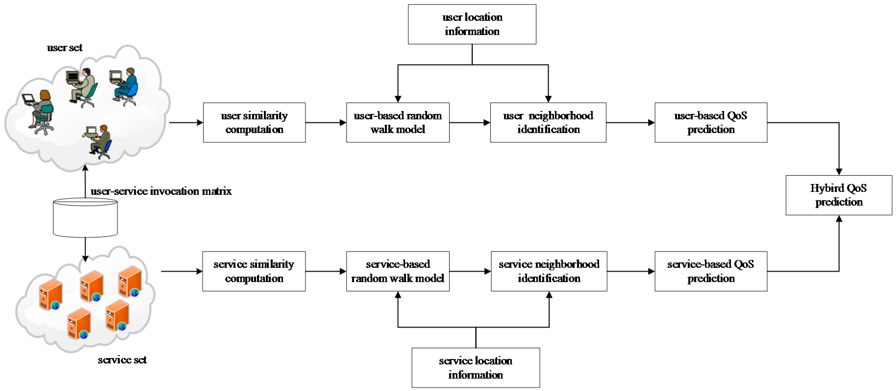
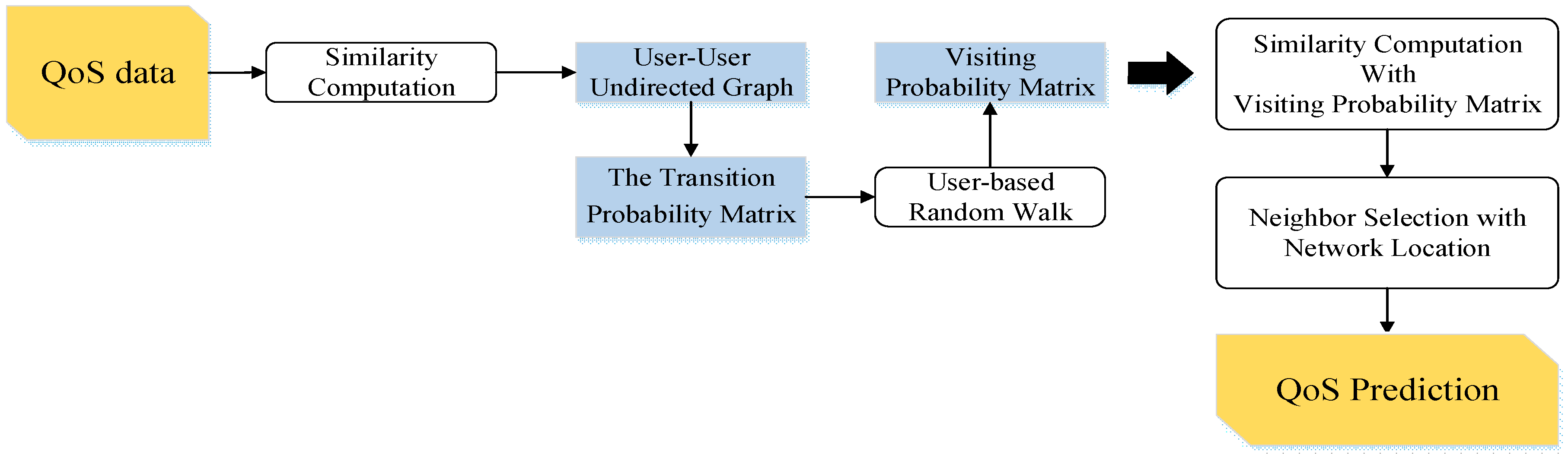
5.1. The QoS Prediction Framework
- The user-based prediction model. This model extends the user-based CF model, which improves the user similarity computation by integrating random walk model, to select similar neighbors. Both the random walk model and neighbor selection are capable of using the network location information. The unknown QoS values are predicted using the QoS records of similar neighbors collaboratively.
- The service-based prediction model. This model extends the service-based CF model, which improves the service similarity computation also by integrating random walk model. Other technical details are similar to those of the user-based prediction model.
- The hybrid model. To further improve the prediction accuracy, our idea is to fully utilize the similar user neighborhood and similar service neighborhood. In this paper, we propose a linear hybrid model, which combines the predicted results of the user-based model and service-based model.
5.2. Direct Similarity Computation
- The fluctuation range of QoS values can be very large. For example, the response time value may be any value in the range of 0 s~20 s or 30 s. If two users receive very different QoS values from the same service, the final similarity can be generated with a large bias.
- In the case that the number of services commonly invoked by two users is small, the similarity computation result tends to be vulnerable. In an extreme case that two users only share one service that is commonly invoked, the similarity result turns to be quite unreliable.
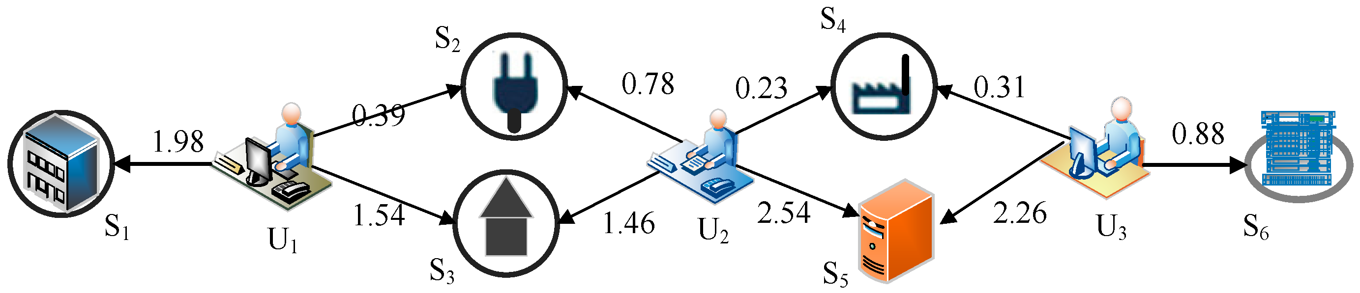
5.3. The Proposed Random Walk Models
5.3.1. The State Transition of Random Walk
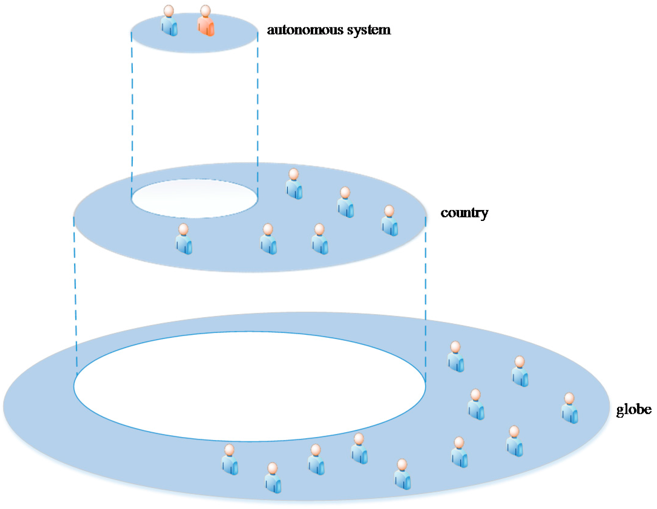
- If user and user are in the same autonomous system, then the set U contains the users of the autonomous system.
- If user and user are in the same country, but not the same autonomous system, then the set U contains the users of the country.
- If user and user are not in the same country or autonomous system, then the set U contains all users.
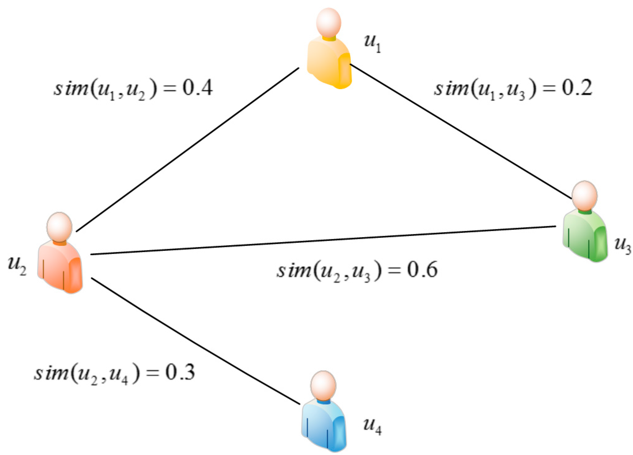
5.3.2. The Transition Probability Matrix
- Continue the walking process along a route with the probability .
- Skip back to the initial node with probability . In this paper, is assigned to 0.85 following the suggestion of Page et al. [35].
5.3.3. Similarity Computation with Visiting Probability Matrix
5.4. Neighborhood Construction and QoS Prediction
5.4.1. Neighbor Selection with Network Location
5.4.2. QoS Prediction and Service Recommendation
User-Based QoS Prediction
Service-Based QoS Prediction
Hybrid QoS Prediction
6. Experiment and Evaluation
- How do the proposed models behave in different data sparsity cases?
- How do the proposed models perform compared to other models?
- How do the parameter λ and K impact the prediction accuracy?
6.1. Dataset
6.2. Evaluation Metric and Parameter Setting
6.3. Prediction Accuracy Comparison
- UserMean: this method uses the average value of each user as the prediction value.
- ItemMean: this method uses the average value of each service as the prediction value.
- UPCC (user-based PCC) [37]: the user-based collaborative filtering algorithm using Pearson correlation coefficient (Resnick et al., 1994).
- IPCC (item-based PCC) [38]: the item-based collaborative filtering algorithm using Pearson correlation coefficient (Sarwar et al., 2001).
- WSRec [36]: This method linearly combines the results of UPCC and IPCC to produce a hybrid result (Zheng et al., 2009).
- LACF [39]: A collaborative filtering algorithm that integrates the location information of users and services (Tang et al., 2012).
- SVD [40]: the singular value decomposition model (Koren et al., 2009).
- The proposed models SL-RW, UL-RW and HL-RW all achieve smaller MAE and NMAE than the baseline models, almost in all cases of training set densities.
- Along with the increase in training set density, the prediction accuracy also becomes higher. The reason is that more training data can provide more invocation records to improve the prediction of similarity computation and neighbor selection.
- The improvement achieved by our models are significant based on the paired t-test (p < 0.001).
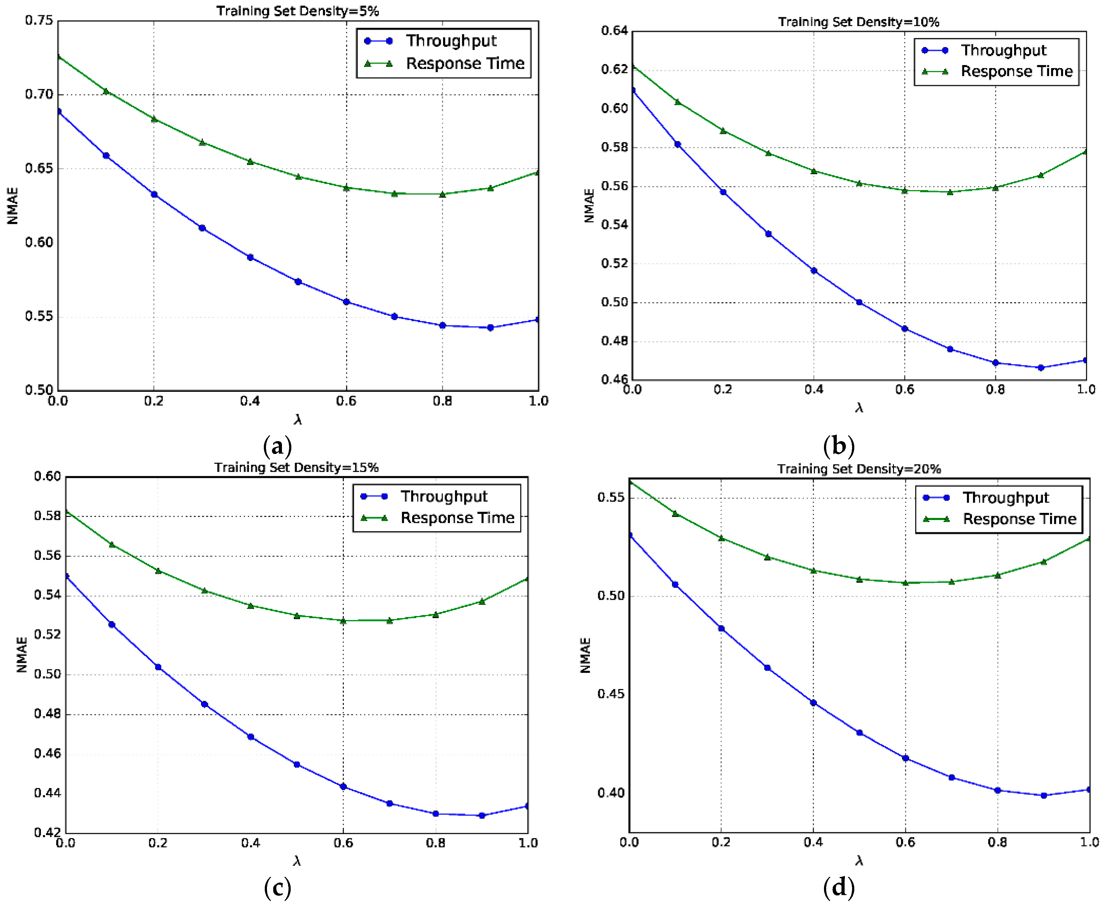
6.4. Impact of λ
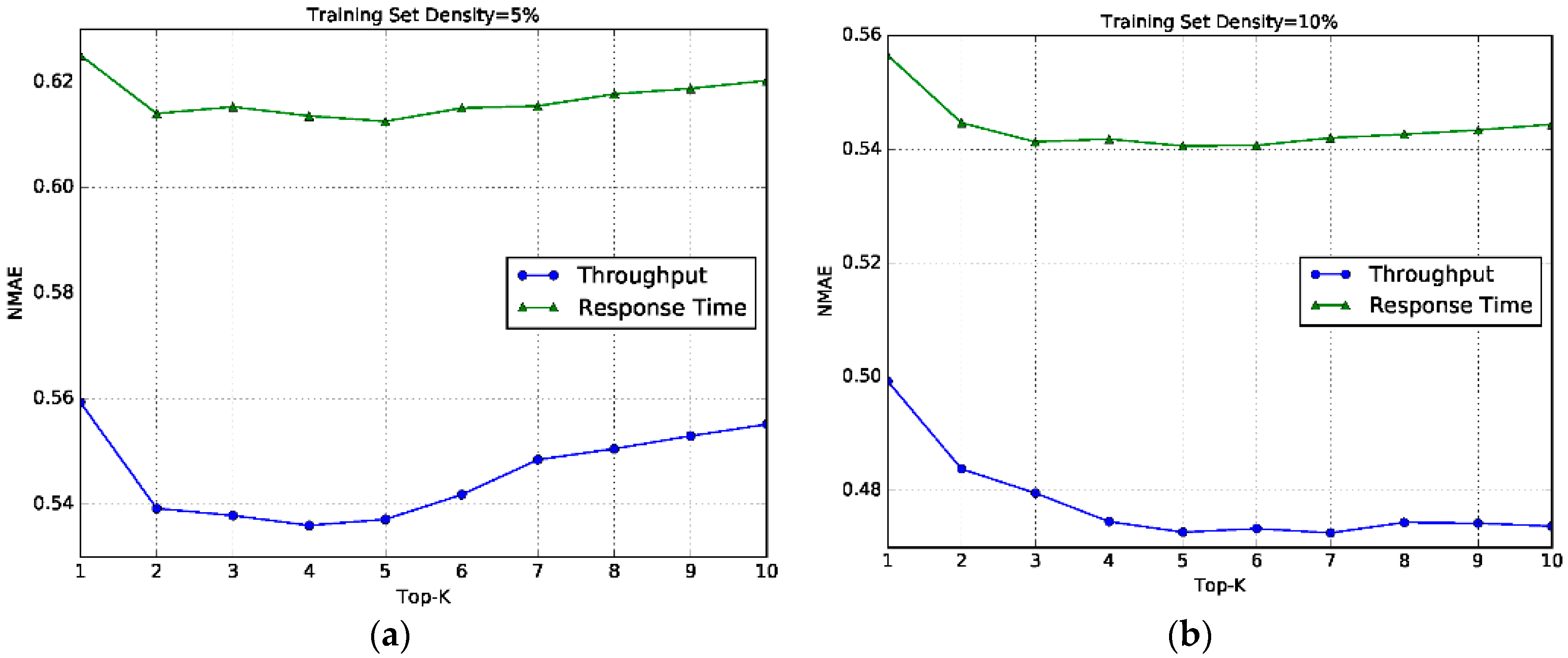
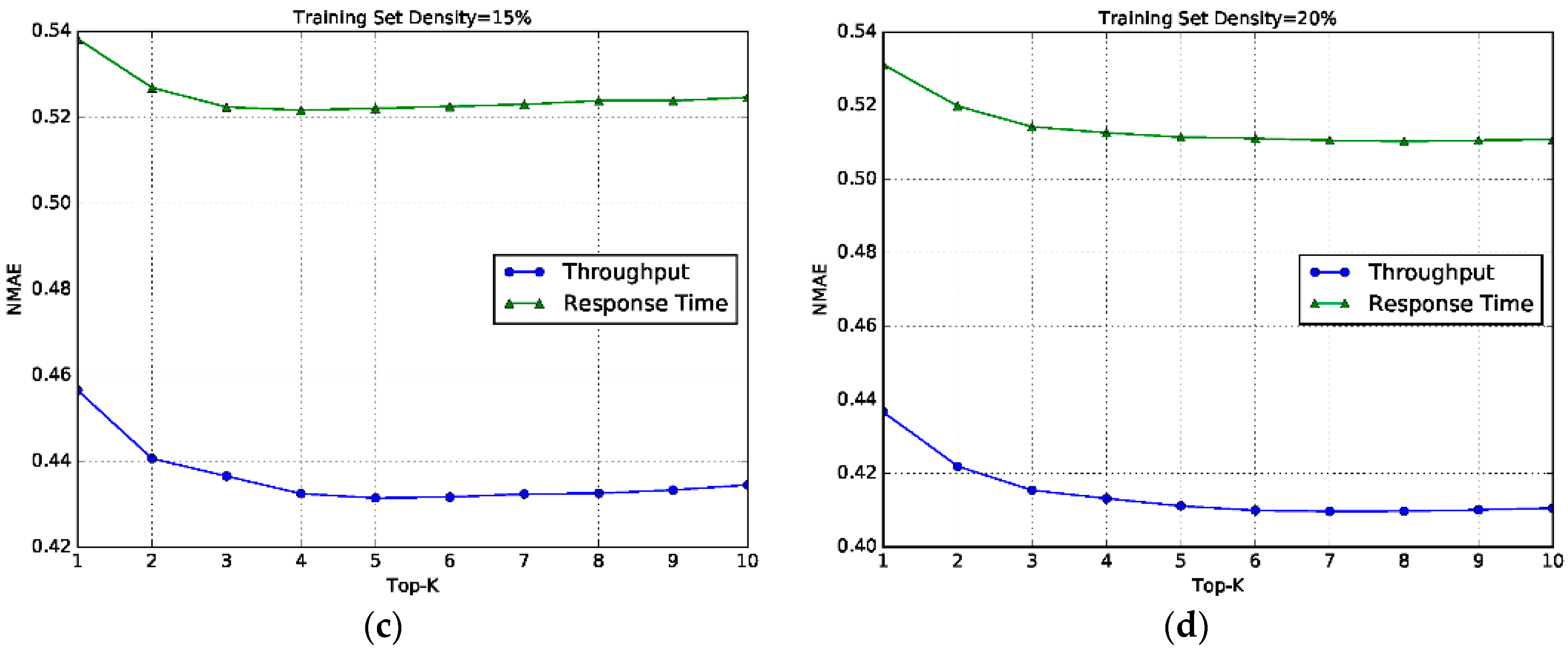
6.5. Impact of K
6.6. Computation Overhead Comparison
7. Discussion and Summary
7.1. Summary of the Motivation
7.2. Discussion on the Network Location
8. Conclusions and Future Work
Acknowledgments
Author Contributions
Conflicts of Interest
References
- Mohammed, A.W.; Xu, Y.; Hu, H.; Agyemang, B. Markov Task Network: A Framework for Service Composition under Uncertainty in Cyber-Physical Systems. Sensors 2016, 16, 1542. [Google Scholar] [CrossRef] [PubMed]
- Stankovic, J.A. Research Directions for Cyber Physical Systems in Wireless and Mobile Healthcare. ACM Trans. Cyber Phys. Syst. 2016, 1. [Google Scholar] [CrossRef]
- Liu, Y.; Peng, Y.; Wang, B.; Yao, S.; Liu, Z. Review on cyber-physical systems. IEEE/CAA J. Autom. Sin. 2017, 4, 27–40. [Google Scholar] [CrossRef]
- Gartner, Inc. Available online: http://www.gartner.com/newsroom/id/3598917 (accessed on 7 February 2017).
- Alrifai, M.; Risse, T. Combining global optimization with local selection for efficient QoS-aware service composition. In Proceedings of the 18th International Conference on World Wide Web, Madrid, Spain, 20–24 April 2009; pp. 881–890. [Google Scholar]
- Haddad, J.E.; Manouvrier, M.; Rukoz, M. TQoS: Transactional and QoS-aware selection algorithm for automatic web service composition. IEEE Trans. Serv. Comput. 2010, 3, 73–85. [Google Scholar] [CrossRef]
- Huang, Y.; Huang, J.; Cheng, B.; He, S.; Chen, J. Time-Aware Service Ranking Prediction in the Internet of Things Environment. Sensors 2017, 17, 974. [Google Scholar] [CrossRef] [PubMed]
- Zheng, Z.; Ma, H.; Lyu, M.R.; King, I. QoS-aware web service recommendation by collaborative filtering. IEEE Trans. Serv. Comput. 2011, 4, 140–152. [Google Scholar] [CrossRef]
- Wu, Q.; Zhu, Q.; Li, P. A neural network based reputation bootstrapping approach for service selection. Enterp. Inf. Syst. 2015, 9, 768–784. [Google Scholar] [CrossRef]
- Jorgensen, P.C. Software Testing: A Craftsmans Approach; CRC Press: Boca Raton, FL, USA, 1995. [Google Scholar]
- Yu, T.; Zhang, Y.; Lin, K.-J. Efficient algorithms for web services selection with end-to-end QoS constraints. ACM Trans. Web (TWEB) 2007, 1, 6. [Google Scholar] [CrossRef]
- Chen, Y.-W.; Xia, X.; Shi, Y.-G. A collaborative filtering recommendation algorithm based on contents’ genome. In Proceedings of the IET International Conference on Information Science and Control Engineering 2012 (ICISCE 2012), Shenzhen, China, 7–9 December 2012; pp. 1–4. [Google Scholar]
- Goldberg, D.; Nichols, D.; Oki, B.M.; Terry, D. Using collaborative filtering to weave an information tapestry. Commun. ACM 1992, 35, 61–70. [Google Scholar] [CrossRef]
- Konstan, J.A.; Miller, B.N.; Maltz, D.; Herlocker, J.L.; Gordon, L.R.; Riedl, J. Grouplens: Applying collaborative filtering to usenet news. Commun. ACM 1997, 40, 77–87. [Google Scholar] [CrossRef]
- Shao, L.; Zhang, J.; Wei, Y.; Zhao, J.; Xie, B.; Mei, H. Personalized QoS prediction for web services via collaborative filtering. In Proceedings of the IEEE International Conference on Web Services (ICWS 2007), Salt Lake City, UT, USA, 9–13 July 2007; pp. 439–446. [Google Scholar]
- Chen, M.; Ma, Y.; Hu, B.; Zhang, L.-J. A ranking-oriented hybrid approach to QoS-aware web service recommendation. In Proceedings of the IEEE International Conference on Services Computing (SCC), New York, NY, USA, 27 June–2 July 2015; pp. 578–585. [Google Scholar]
- Jiang, Y.; Liu, J.; Tang, M.; Liu, X. An effective web service recommendation method based on personalized collaborative filtering. In Proceedings of the 2011 IEEE International Conference on Web Services (ICWS), Washington, DC, USA, 4–9 July 2011; pp. 211–218. [Google Scholar]
- Fan, X.; Hu, Y.; Zhang, R. Context-aware web services recommendation based on user preference. In Proceedings of the Asia-Pacific Services Computing Conference (APSCC), Fuzhou, China, 4–6 December 2014; pp. 55–61. [Google Scholar]
- Chen, X.; Liu, X.; Huang, Z.; Sun, H. RegionKNN: A scalable hybrid collaborative filtering algorithm for personalized web service recommendation. In Proceedings of the IEEE International Conference on Web Services (ICWS), Miami, FL, USA, 5–10 July 2010; pp. 9–16. [Google Scholar]
- Liu, J.; Tang, M.; Zheng, Z.; Liu, X.; Lyu, S. Location-Aware and Personalized Collaborative Filtering for Web Service Recommendation Preprint; IJIERT: Maharashtra, India, 2015. [Google Scholar]
- Yu, D.; Liu, Y.; Xu, Y.; Yin, Y. Personalized QoS prediction for web services using latent factor models. In Proceedings of the International Conference on Services Computing (SCC), Anchorage, AK, USA, 27 June–2 July 2014; pp. 107–114. [Google Scholar]
- Yao, L.; Sheng, Q.Z.; Segev, A.; Yu, J. Recommending web services via combining collaborative filtering with content-based features. In Proceedings of the International Conference on Web Services (ICWS), Santa Clara, CA, USA, 28 June–3 July 2013; pp. 42–49. [Google Scholar]
- He, P.; Zhu, J.; Zheng, Z.; Xu, J.; Lyu, M.R. Location-Based Hierarchical Matrix Factorization for Web Service Recommendation. In Proceedings of the IEEE International Conference on Web Services, Anchorage, AK, USA, 27 June–2 July 2014; pp. 297–304. [Google Scholar]
- Yu, C.; Huang, L. Time-Aware Collaborative Filtering for QoS-Based Service Recommendation. In Proceedings of the IEEE International Conference on Web Services, Anchorage, AK, USA, 27 June–2 July 2014; pp. 265–272. [Google Scholar]
- Lee, K.; Park, J.; Baik, J. Location-Based Web Service QoS Prediction via Preference Propagation for Improving Cold Start Problem. In Proceedings of the IEEE International Conference on Web Services, New York, NY, USA, 27 June–2 July 2015; pp. 177–184. [Google Scholar]
- Qi, K.; Hu, H.; Song, W.; Ge, J.; Lü, J. Personalized QoS Prediction via Matrix Factorization Integrated with Neighborhood Information. In Proceedings of the IEEE International Conference on Services Computing, New York, NY, USA, 27 June–2 July 2015; pp. 186–193. [Google Scholar]
- Ma, Y.; Wang, S.; Yang, F.; Chang, R.N. Predicting QoS Values via Multi-dimensional QoS Data for Web Service Recommendations. In Proceedings of the IEEE International Conference on Web Services, New York, NY, USA, 27 June–2 July 2015; pp. 249–256. [Google Scholar]
- Wu, C.; Qiu, W.; Zheng, Z.; Wang, X.; Yang, X. QoS Prediction of Web Services Based on Two-Phase K-Means Clustering. In Proceedings of the IEEE International Conference on Web Services, New York, NY, USA, 27 June–2 July 2015; pp. 161–168. [Google Scholar]
- Zhou, Z.; Wang, B.; Guo, J.; Pan, J. QoS-Aware Web Service Recommendation Using Collaborative Filtering with PGraph. In Proceedings of the IEEE International Conference on Web Services, New York, NY, USA, 27 June–2 July 2015; pp. 392–399. [Google Scholar]
- Zhang, Z.; Cuff, P.; Kulkarni, S. Iterative collaborative filtering for recommender systems with sparse data. In Proceedings of the International Workshop on Machine Learning for Signal Processing, Santander, Spain, 23–26 September 2012; pp. 1–6. [Google Scholar]
- Yildirim, H.; Krishnamoorthy, M.S. A random walk method for alleviating the sparsity problem in collaborative filtering. In Proceedings of the ACM conference on Recommender systems (RecSys), Lausanne, Switzerland, 23–25 October 2008; pp. 131–138. [Google Scholar]
- Huang, B.; Li, C.; Tao, F. A chaos control optimal algorithm for QoS-based service composition selection in cloud manufacturing system. Enterp. Inf. Syst. 2014, 8, 445–463. [Google Scholar] [CrossRef]
- Xie, Q.; Zhao, S.; Zheng, Z.; Zhu, J.; Lyu, M.R. Asymmetric Correlation Regularized Matrix Factorization for Web Service Recommendation. In Proceedings of the IEEE International Conference on Web Services, San Francisco, CA, USA, 27 June–2 July 2016; pp. 204–211. [Google Scholar]
- Gilks, W.R. Markov chain monte carlo. In Encyclopedia of Biostatistics; Wiley Online Library: Hoboken, NJ, USA, 2005. [Google Scholar]
- Page, L.; Brin, S.; Motwani, R.; Winograd, T. The Pagerank Citation Ranking: Bringing Order to the Web; Stanford InfoLab Publication Server: Stanford, CA, USA, 1999. [Google Scholar]
- Zheng, Z.; Ma, H.; Lyu, M.R.; King, I. Wsrec: A collaborative filtering based web service recommender system. In Proceedings of the IEEE International Conference on Web Services, Los Angeles, CA, USA, 6–10 July 2009; pp. 437–444. [Google Scholar]
- Resnick, P.; Iacovou, N.; Suchak, M.; Bergstrom, P.; Riedl, J. Grouplens: An open architecture for collaborative filtering of netnews. In Proceedings of the 1994 ACM conference on Computer supported cooperative work, Chapel Hill, NC, USA, 22–26 October 1994; pp. 175–186. [Google Scholar]
- Sarwar, B.; Karypis, G.; Konstan, J.; Riedl, J. Item-based collaborative filtering recommendation algorithms. In Proceedings of the 10th international conference on World Wide Web, Hong Kong, China, 1–5 May 2001; pp. 285–295. [Google Scholar]
- Tang, M.; Jiang, Y.; Liu, J.; Liu, X. Location-aware collaborative filtering for QoS-based service recommendation. In Proceedings of the International Conference on Web Services (ICWS), Honolulu, HI, USA, 24–29 June 2012; pp. 202–209. [Google Scholar]
- Koren, Y.; Bell, R.; Volinsky, C. Matrix factorization techniques for recommender systems. Computer 2009, 42, 30–37. [Google Scholar] [CrossRef]


| Service 1 | Service 2 | Service 3 | Service 4 | Servcie 5 | |
|---|---|---|---|---|---|
| User 1 | ? | ? | 1.74 | ? | ? |
| User 2 | 1.28 | ? | ? | ? | 3.14 |
| User 3 | ? | ? | ? | 0.89 | ? |
| User 4 | 3.21 | ? | ? | ? | 1.35 |
| Attributes | Numbers |
|---|---|
| the number of users | 339 |
| the number of services | 5828 |
| the number of invocation records | 1,974,675 |
| the number of user countries | 30 |
| the number of service countries | 73 |
| average value of response time | 0.81 |
| average value of throughput | 44.03 |
| Model | Training Set Density (TD)—Response Time Dataset | |||||||
|---|---|---|---|---|---|---|---|---|
| TD = 5% | TD = 10% | TD = 15% | TD = 20% | |||||
| MAE | NMAE | MAE | NMAE | MAE | NMAE | MAE | NMAE | |
| UserMean | 0.8818 | 1.0873 | 0.8794 | 1.0832 | 0.8788 | 1.0832 | 0.8785 | 1.0837 |
| ItemMean | 0.7223 | 0.8904 | 0.7082 | 0.8723 | 0.7014 | 0.8642 | 0.7002 | 0.8630 |
| UPCC | 0.7568 | 0.9332 | 0.7137 | 0.8802 | 0.6311 | 0.7779 | 0.5919 | 0.7298 |
| IPCC | 0.7184 | 0.8851 | 0.7345 | 0.9061 | 0.6991 | 0.8617 | 0.6503 | 0.8013 |
| WSRec | 0.6832 | 0.9409 | 0.6306 | 0.8390 | 0.6137 | 0.7810 | 0.6020 | 0.7545 |
| LACF | 0.6575 | 0.8476 | 0.6398 | 0.8011 | 0.6023 | 0.7425 | 0.5723 | 0.7055 |
| SVD | 0.5793 | 0.7142 | 0.5683 | 0.7006 | 0.5430 | 0.6704 | 0.5328 | 0.6568 |
| SL-RW | 0.5885 | 0.6054 | 0.5036 | 0.5609 | 0.4763 | 0.5254 | 0.4598 | 0.5026 |
| UL-RW | 0.5289 | 0.6481 | 0.4667 | 0.5782 | 0.4490 | 0.5489 | 0.4302 | 0.5297 |
| HL-RW | 0.5172 | 0.6374 | 0.4604 | 0.5580 | 0.4316 | 0.5274 | 0.4128 | 0.5069 |
| Model | Training Set Density (TD)—Throughput Dataset | |||||||
|---|---|---|---|---|---|---|---|---|
| TD = 5% | TD = 10% | TD = 15% | TD = 20% | |||||
| MAE | NMAE | MAE | NMAE | MAE | NMAE | MAE | NMAE | |
| UserMean | 51.032 | 1.1644 | 52.822 | 1.1665 | 51.051 | 1.1597 | 51.490 | 1.1584 |
| ItemMean | 32.386 | 0.7389 | 32.226 | 0.7117 | 31.889 | 0.7244 | 31.895 | 0.7175 |
| UPCC | 29.157 | 0.6653 | 25.464 | 0.5624 | 22.270 | 0.5059 | 20.479 | 0.4607 |
| IPCC | 47.748 | 1.0894 | 47.098 | 1.0401 | 40.802 | 0.9321 | 39.505 | 0.8887 |
| WSRec | 30.502 | 0.6783 | 26.532 | 0.5892 | 22.025 | 0.5048 | 20.213 | 0.4587 |
| LACF | 28.612 | 0.6543 | 25.451 | 0.5714 | 22.403 | 0.5123 | 20.105 | 0.4439 |
| SVD | 35.972 | 0.7072 | 32.563 | 0.6753 | 31.852 | 0.6528 | 29.774 | 0.6303 |
| SL-RW | 29.449 | 0.6889 | 27.170 | 0.6098 | 24.237 | 0.5499 | 23.438 | 0.5314 |
| UL-RW | 23.279 | 0.5352 | 20.740 | 0.4669 | 19.123 | 0.4349 | 17.888 | 0.4071 |
| HL-RW | 23.263 | 0.5348 | 20.428 | 0.4511 | 18.934 | 0.4315 | 17.315 | 0.4028 |
| Model | Training Set Density (TD)—Response Time Dataset | |||
|---|---|---|---|---|
| TD = 5% | TD = 10% | TD = 15% | TD = 20% | |
| Running Time (s) | Running Time (s) | Running Time (s) | Running Time (s) | |
| UPCC | 22.139 | 43.727 | 77.589 | 136.889 |
| IPCC | 358.659 | 612.326 | 941.629 | 1243.632 |
| WSRec | 383.324 | 659.884 | 1012.265 | 1372.266 |
| LACF | 267.514 | 483.721 | 831.260 | 1152.265 |
| SVD | 399.347 | 811.453 | 1232.871 | 1982.789 |
| UL-RW | 31.403 | 59.166 | 92.570 | 148.618 |
| SL-RW | 383.226 | 726.570 | 1053.269 | 1358.321 |
| HL-RW | 418.009 | 789.102 | 1151.890 | 1509.598 |
© 2017 by the authors. Licensee MDPI, Basel, Switzerland. This article is an open access article distributed under the terms and conditions of the Creative Commons Attribution (CC BY) license (http://creativecommons.org/licenses/by/4.0/).
Share and Cite
Yin, Y.; Yu, F.; Xu, Y.; Yu, L.; Mu, J. Network Location-Aware Service Recommendation with Random Walk in Cyber-Physical Systems. Sensors 2017, 17, 2059. https://doi.org/10.3390/s17092059
Yin Y, Yu F, Xu Y, Yu L, Mu J. Network Location-Aware Service Recommendation with Random Walk in Cyber-Physical Systems. Sensors. 2017; 17(9):2059. https://doi.org/10.3390/s17092059
Chicago/Turabian StyleYin, Yuyu, Fangzheng Yu, Yueshen Xu, Lifeng Yu, and Jinglong Mu. 2017. "Network Location-Aware Service Recommendation with Random Walk in Cyber-Physical Systems" Sensors 17, no. 9: 2059. https://doi.org/10.3390/s17092059
APA StyleYin, Y., Yu, F., Xu, Y., Yu, L., & Mu, J. (2017). Network Location-Aware Service Recommendation with Random Walk in Cyber-Physical Systems. Sensors, 17(9), 2059. https://doi.org/10.3390/s17092059