An Ensemble Deep Convolutional Neural Network Model with Improved D-S Evidence Fusion for Bearing Fault Diagnosis


Abstract
:1. Introduction
2. Materials and Methods
2.1. Improved D-S Evidence Theory for Information Fusion
2.1.1. Preliminaries
2.1.2. The Improved D-S Evidence Theory
- (1)
- Calculate the distances matrix D and its elements among raw evidences.
- (2)
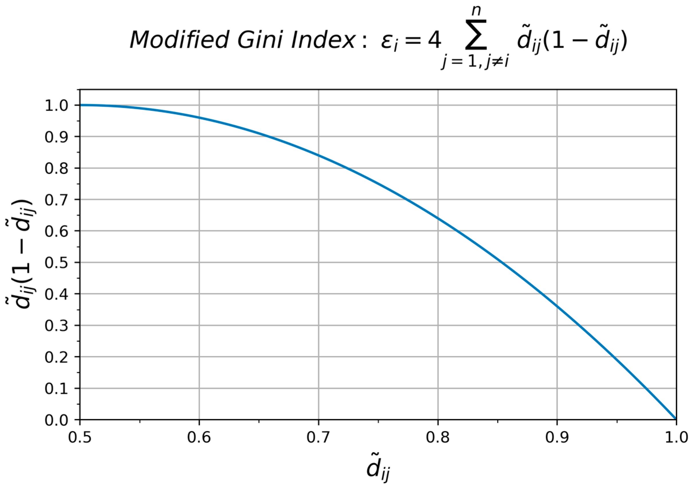
- Calculate the evidence credibility using the modified Gini Index expression.
- (3)
- Calculate the probability of weighted proposition m*(A).
- (4)
- Calculate the final evidence through scaling and normalizing for validation.
- (5)
- Calculate the maximum and select the relevant proposition as the diagnosis result.
2.2. The IDSCNN Ensemble CNN Model for Bearing Fault Diagnosis
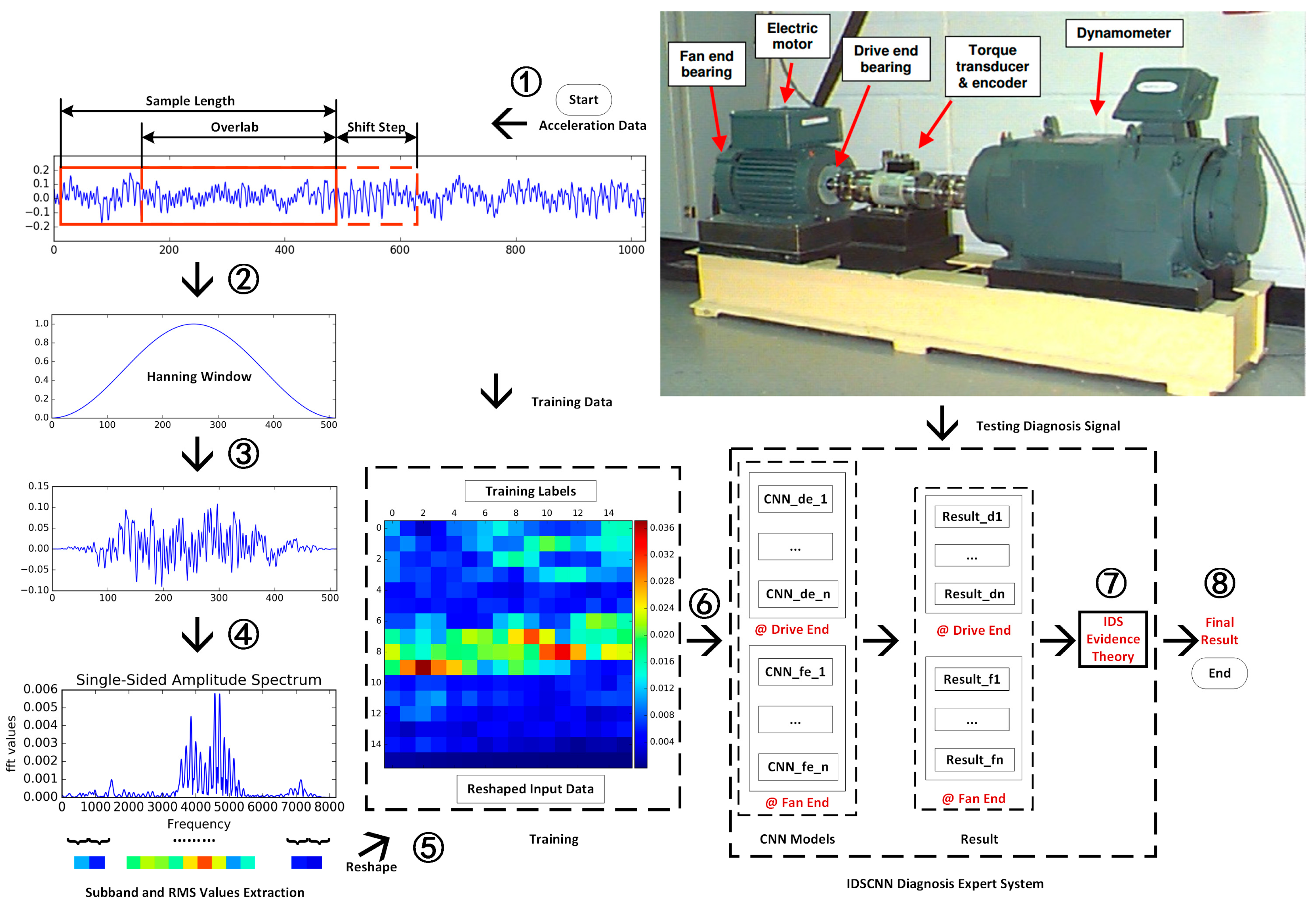
2.2.1. Data Preparation
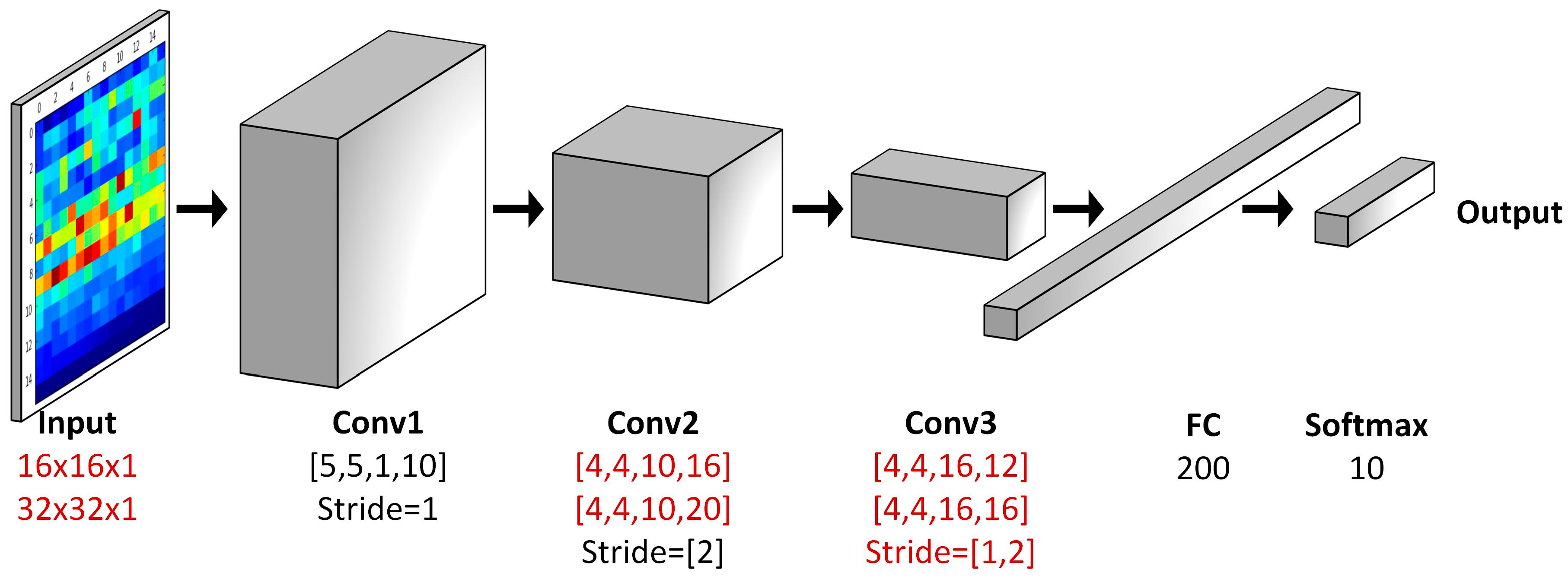
2.2.2. The IDSCNN Model based on CNNs
2.2.3. Model Testing
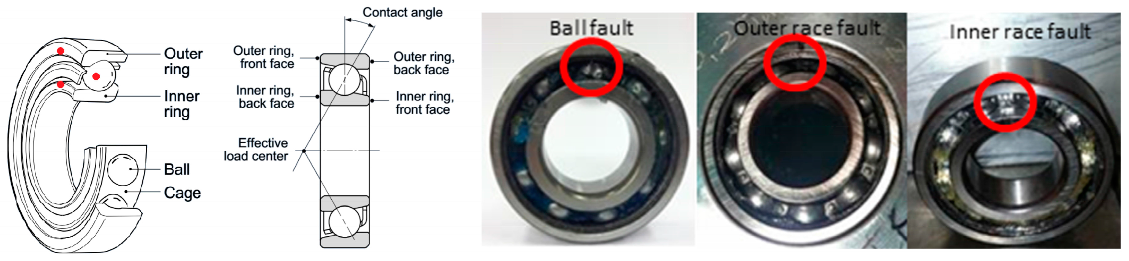
2.3. Experiment Set-Up
3. Results
3.1. Evaluation of the Improved D-S Evidence (IDS) Fusion Algorithm
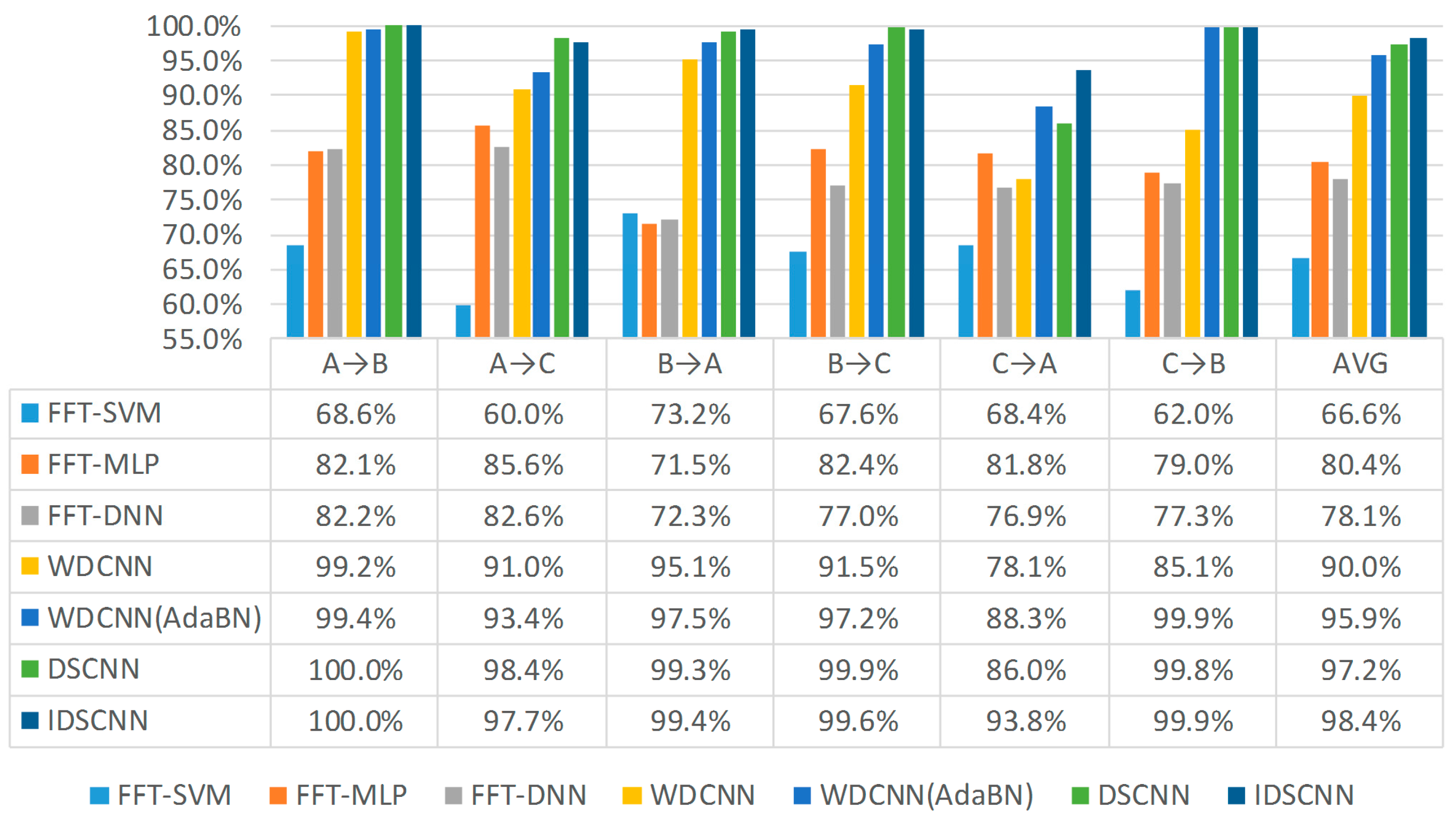
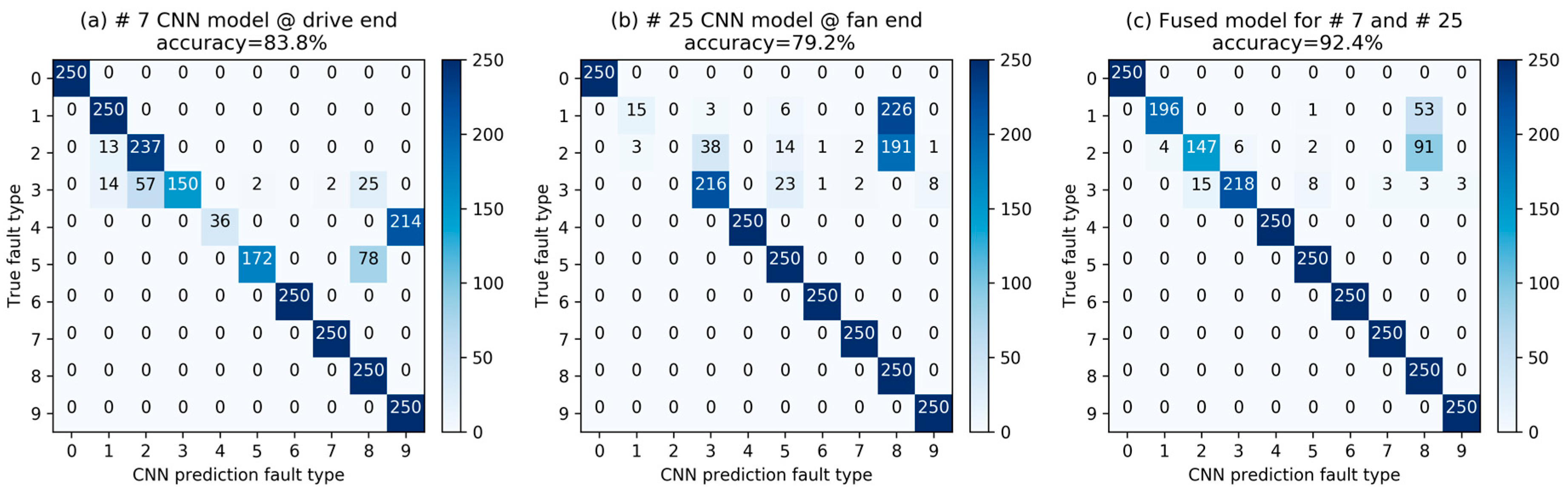
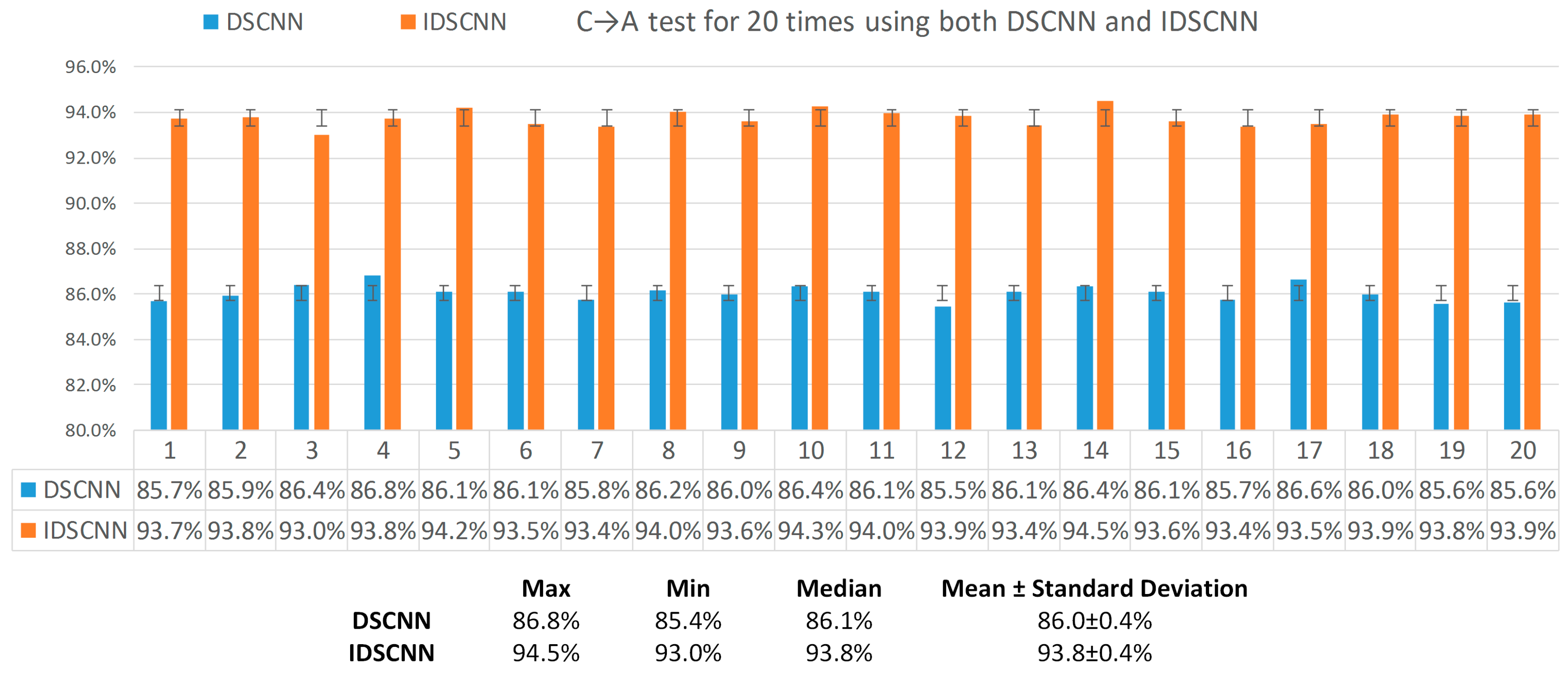
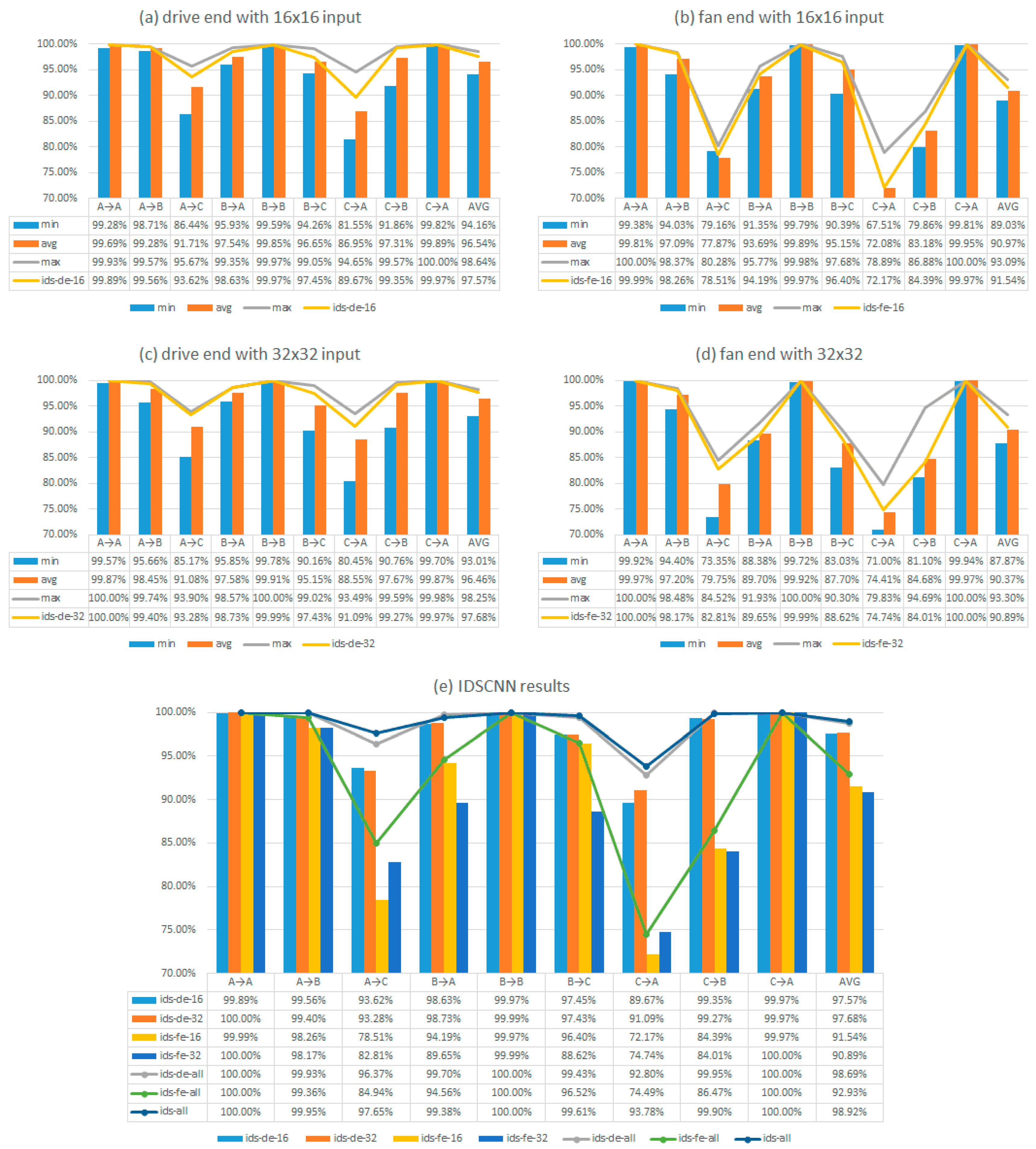
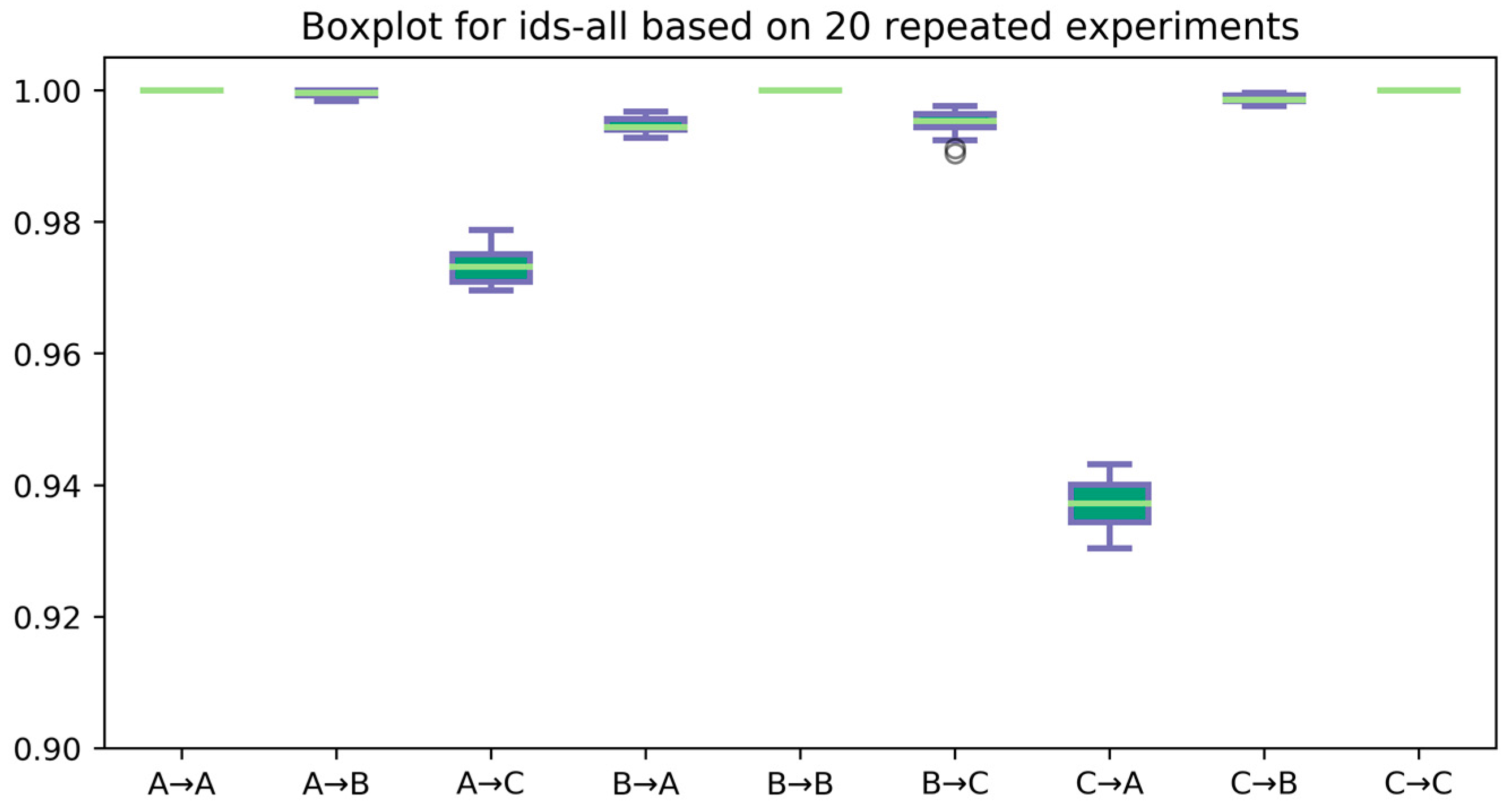
3.2. Evaluation of IDSCNN for Bearing Fault Diagnosis on the CWRU Dataset
4. Conclusions
Acknowledgments
Author Contributions
Conflicts of Interest
References
- Gelman, L.; Murray, B.; Patel, T.H.; Thomson, A. Vibration diagnostics of rolling bearings by novel nonlinear non-stationary wavelet bicoherence technology. Eng. Struct. 2014, 80, 514–520. [Google Scholar] [CrossRef]
- Jena, D.P.; Panigrahi, S.N. Automatic gear and bearing fault localization using vibration and acoustic signals. Appl. Acoust. 2015, 98, 20–33. [Google Scholar] [CrossRef]
- Peng, E.G.; Liu, Z.L.; Zhou, X.C.; Zhao, M.Y.; Lan, F. Application of Vibration and Noise Analysis in Water-Lubricated Rubber Bearings Fault Diagnosis. Adv. Mater. Res. 2011, 328–330, 1995–1999. [Google Scholar] [CrossRef]
- Janssens, O.; Schulz, R.; Slavkovikj, V.; Stockman, K.; Loccufier, M.; Walle, R.V.D.; Hoecke, S.V. Thermal image based fault diagnosis for rotating machinery. Inf. Phys. Technol. 2015, 73, 78–87. [Google Scholar] [CrossRef]
- Chen, J.; Zi, Y.; He, Z.; Wang, X. Adaptive redundant multiwavelet denoising with improved neighboring coefficients for gearbox fault detection. Mech. Syst. Signal Proc. 2013, 38, 549–568. [Google Scholar] [CrossRef]
- Safin, N.R.; Prakht, V.A.; Dmitrievskii, V.A.; Dmitrievskii, A.A. Diagnosis of Bearing Faults of Induction Motors by Spectral Analysis of Stator Currents. Adv. Mater. Res. 2014, 1070–1072, 1187–1190. [Google Scholar] [CrossRef]
- Yang, J.; Zhang, J.; Zhang, G.; Liu, Y. Fault Diagnosis of Transmission Rolling Bearing Based on Wavelet Analysis and Binary Tree Support Vector Machine. Int. J. Digit. Content Technol. Its Appl. 2013, 6, 580. [Google Scholar]
- Mohanty, S.; Gupta, K.K.; Raju, K.S.; Singh, A.; Snigdha, S. Vibro acoustic signal analysis in fault finding of bearing using Empirical Mode Decomposition. Prceedings of the International Conference on Advanced Electronic Systems, Pilani, India, 21–23 September 2013; pp. 29–33. [Google Scholar]
- Luo, J.; Yu, D.; Liang, M. A kurtosis-guided adaptive demodulation technique for bearing fault detection based on tunable-Q wavelet transform. Meas. Sci. Technol. 2013, 24, 055009. [Google Scholar] [CrossRef]
- Cui, L.; Wu, N.; Ma, C.; Wang, H. Quantitative fault analysis of roller bearings based on a novel matching pursuit method with a new step-impulse dictionary. Mech. Syst. Signal Proc. 2016, 68, 34–43. [Google Scholar] [CrossRef]
- Misra, M.; Yue, H.H.; Qin, S.J.; Ling, C. Multivariate process monitoring and fault diagnosis by multi-scale PCA. Comput. Chem. Eng. 2002, 26, 1281–1293. [Google Scholar] [CrossRef]
- Widodo, A.; Yang, B.S. Application of nonlinear feature extraction and support vector machines for fault diagnosis of induction motors. Exp. Syst. Appl. 2007, 33, 241–250. [Google Scholar] [CrossRef]
- Muralidharan, A.; Sugumaran, V.; Soman, K.P. Bearing Fault Diagnosis Using Vibration Signals by Variational Mode Decomposition and Naïve Bayes Classifier. Int. J. Robot. Autom. 2016, 1, 1–14. [Google Scholar]
- Pandya, D.H.; Upadhyay, S.H.; Harsha, S.P. Fault diagnosis of rolling element bearing with intrinsic mode function of acoustic emission data using APF-KNN. Exp. Syst. Appl. 2013, 40, 4137–4145. [Google Scholar] [CrossRef]
- Hajnayeb, A.; Ghasemloonia, A.; Khadem, S.E.; Moradi, M.H. Application and comparison of an ANN-based feature selection method and the genetic algorithm in gearbox fault diagnosis. Exp. Syst. Appl. 2011, 38, 10205–10209. [Google Scholar] [CrossRef]
- FernáNdez-Francos, D.; MartíNez-Rego, D.; Fontenla-Romero, O.; Alonso-Betanzos, A. Automatic bearing fault diagnosis based on one-class v-SVM. Comput. Ind. Eng. 2013, 64, 357–365. [Google Scholar] [CrossRef]
- Jia, G.; Yuan, S.; Tang, C.; Xiong, J. Fault diagnosis of roller bearing using feedback EMD and decision tree. Prceedings of the International Conference on Electric Information and Control Engineering, Wuhan, China, 15–17 April 2011; pp. 4212–4215. [Google Scholar]
- Peng, H.W.; Chiang, P.J. Control of mechatronics systems: Ball bearing fault diagnosis using machine learning techniques. Prceedings of the 8th Asian Control Conference, Kaohsiung, Taiwan, 15–18 May 2011; pp. 175–180. [Google Scholar]
- Jedliński, Ł.; Jonak, J. Early fault detection in gearboxes based on support vector machines and multilayer perceptron with a continuous wavelet transform. Appl. Soft Comput. 2015, 30, 636–641. [Google Scholar] [CrossRef]
- Kankar, P.K.; Sharma, S.C.; Harsha, S.P. Fault diagnosis of rolling element bearing using cyclic autocorrelation and wavelet transform. Neurocomputing 2013, 110, 9–17. [Google Scholar] [CrossRef]
- Zhang, X.; Qiu, D.; Chen, F. Support vector machine with parameter optimization by a novel hybrid method and its application to fault diagnosis. Neurocomputing 2015, 149, 641–651. [Google Scholar] [CrossRef]
- Ji, N.N.; Zhang, J.S.; Zhang, C.X. A sparse-response deep belief network based on rate distortion theory. Pattern Recognit. 2014, 47, 3179–3191. [Google Scholar] [CrossRef]
- Leng, B.; Zhang, X.; Yao, M.; Xiong, Z. A 3D model recognition mechanism based on deep Boltzmann machines. Neurocomputing 2015, 151, 593–602. [Google Scholar] [CrossRef]
- Katayama, K.; Ando, M.; Horiguchi, T. Model of MT and MST areas using an autoencoder. Physics A 2003, 322, 531–545. [Google Scholar] [CrossRef]
- Zhang, W.; Li, R.; Deng, H.; Li, W.; Lin, W.; Ji, S.; Shen, D. Deep Convolutional Neural Networks for Multi-Modality Isointense Infant Brain Image Segmentation. Neuroimage 2015, 108, 214–224. [Google Scholar] [CrossRef] [PubMed]
- Guo, X.; Chen, L.; Shen, C. Hierarchical adaptive deep convolution neural network and its application to bearing fault diagnosis. Measurement 2016, 93, 490–502. [Google Scholar] [CrossRef]
- Chen, Z.Q.; Li, C.; Sanchez, R.V. Gearbox Fault Identification and Classification with Convolutional Neural Networks. Shock Vib. 2015, 2015, 1–10. [Google Scholar] [CrossRef]
- Ince, T.; Kiranyaz, S.; Eren, L.; Askar, M.; Gabbouj, M. Real-time motor fault detection by 1-d convolutional neural networks. IEEE Trans. Ind. Electron. 2016, 63, 7067–7075. [Google Scholar] [CrossRef]
- Tran, V.T.; Althobiani, F.; Ball, A. An approach to fault diagnosis of reciprocating compressor valves using Teager–Kaiser energy operator and deep belief networks. Exp. Syst. Appl. 2014, 41, 4113–4122. [Google Scholar] [CrossRef]
- Yager, R.R. On the Dempster-Shafer framework and new combination rules. Inf. Sci. 1987, 41, 93–137. [Google Scholar] [CrossRef]
- Hégarat-Mascle, S.L.; Bloch, I.; Vidal-Madjar, D. Application of Dempster-Shafer evidence theory to unsupervised classification in multisource remote sensing. Geosci. Remote Sens. 1997, 35, 1018–1031. [Google Scholar] [CrossRef]
- Li, Y.-B.; Wang, N.; Zhou, C. Based on D-S evidence theory of information fusion improved method. Prceedings of the International Conference on Computer Application and System Modeling, Taiyuan, China, 22–24 October 2010; pp. V1:416–V1:419. [Google Scholar]
- Dou, Z.; Xu, X.; Lin, Y.; Zhou, R. Application of D-S Evidence Fusion Method in the Fault Detection of Temperature Sensor. Math. Probl. Eng. 2014, 2014, 1–6. [Google Scholar] [CrossRef]
- Hui, K.H.; Meng, H.L.; Leong, M.S.; Al-Obaidi, S.M. Dempster-Shafer evidence theory for multi-bearing faults diagnosis. Eng. Appl. Artif. Intell. 2017, 57, 160–170. [Google Scholar] [CrossRef]
- Browne, F.; Rooney, N.; Liu, W.; Bell, D. Integrating textual analysis and evidential reasoning for decision making in engineering design. Knowl. Based Syst. 2013, 52, 165–175. [Google Scholar] [CrossRef]
- Avci, E. A new method for expert target recognition system: Genetic wavelet extreme learning machine (GAWELM). Exp. Syst. Appl. 2013, 40, 3984–3993. [Google Scholar] [CrossRef]
- Dong, G.; Kuang, G. Target Recognition via Information Aggregation Through Dempster–Shafer’s Evidence Theory. IEEE Geosci. Remote Sens. Lett. 2015, 12, 1247–1251. [Google Scholar] [CrossRef]
- Xing, H.; Hua, G.; Han, Y.; Liu, C.; Dang, Y. Quantitative MMM evaluation of weld levels based on information entropy and DS evidence theory. Chin. J. Sci. Instrum. 2016, 37, 610–616. [Google Scholar]
- Kang, J.; Gu, Y.B.; Li, Y.B. Multi-sensor information fusion algorithm based on DS evidence theory. J. Chin. Inert. Technol. 2012, 20, 670–673. [Google Scholar]
- Li, Y.; Chen, J.; Ye, F.; Liu, D. The Improvement of DS Evidence Theory and Its Application in IR/MMW Target Recognition. J. Sens. 2015, 2016, 1–15. [Google Scholar] [CrossRef]
- AbuMahfouz, I.A. A comparative study of three artificial neural networks for the detection and classification of gear faults. Int. J. Gen. Syst. 2005, 34, 261–277. [Google Scholar] [CrossRef]
- Smith, W.A.; Randall, R.B. Rolling element bearing diagnostics using the Case Western Reserve University data: A benchmark study. Mech. Syst. Signal Proc. 2015, 64–65, 100–131. [Google Scholar] [CrossRef]
- Case Western Reserve University Bearing Data Center Website. Available online: http://csegroups.case.edu/bearingdatacenter/home (accessed on 31 June 2017).
- Yager, R.R. On the aggregation of prioritized belief structures. IEEE Trans. Syst. Man Cybern. Part A 2002, 26, 708–717. [Google Scholar] [CrossRef]
- Sun, Q.; Ye, X.; Gu, W. A New Combination Rules of Evidence Theory. Acta Electron. Sin. 2000, 28, 117–119. [Google Scholar]
- Murphy, C.K. Combining belief functions when evidence conflicts. Decis. Support Syst. 2000, 29, 1–9. [Google Scholar] [CrossRef]
- Deng, Y.; Shi, W.K.; Zhu, Z.F. Efficient combination approach of conflict evidence. J. Infrared Millim. Waves 2004, 23, 27–32. [Google Scholar]
- Jia, F.; Lei, Y.; Lin, J.; Zhou, X.; Lu, N. Deep neural networks: A promising tool for fault characteristic mining and intelligent diagnosis of rotating machinery with massive data. Mech. Syst. Signal Proc. 2016, 72–73, 303–315. [Google Scholar] [CrossRef]
- Zhang, W.; Peng, G.; Li, C.; Chen, Y.; Zhang, Z. A New Deep Learning Model for Fault Diagnosis with Good Anti-Noise and Domain Adaptation Ability on Raw Vibration Signals. Sensors 2017, 17, 425. [Google Scholar] [CrossRef] [PubMed]


| Paradoxes | Evidences | Propositions | ||||
|---|---|---|---|---|---|---|
| A | B | C | D | E | ||
| Complete conflict paradox | m1 | 1 | 0 | 0 | - | - |
| m2 | 0 | 1 | 0 | - | - | |
| m3 | 0.8 | 0.1 | 0.1 | - | - | |
| m4 | 0.5 | 0.2 | 0.3 | - | - | |
| 0 trust paradox | m1 | 0.5 | 0.2 | 0.3 | - | - |
| m2 | 0.5 | 0.2 | 0.3 | - | - | |
| m3 | 0 | 0.9 | 0.1 | - | - | |
| m4 | 0.5 | 0 | 0.3 | - | - | |
| 1 trust paradox | m1 | 0.9 | 0.1 | 0 | - | - |
| m2 | 0 | 0.1 | 0.9 | - | - | |
| m3 | 0.1 | 0.15 | 0.75 | - | - | |
| m4 | 0.1 | 0.15 | 0.75 | - | - | |
| High conflict paradox | m1 | 0.7 | 0.1 | 0.1 | 0 | 0.1 |
| m2 | 0 | 0.5 | 0.2 | 0.1 | 0.2 | |
| m3 | 0.6 | 0.1 | 0.15 | 0 | 0.15 | |
| m4 | 0.55 | 0.1 | 0.1 | 0.15 | 0.1 | |
| m5 | 0.6 | 0.1 | 0.2 | 0 | 0.1 | |
| Parameter Setting | |||||
|---|---|---|---|---|---|
| No | Input | C1 | C2 | C3 | Stride |
| 1 | 16 × 16 × 1 | [5,5,1,10] | [4,4,10,16] | [4,4,16,12] | (1,2,1) |
| 2 | 16 × 16 × 1 | [5,5,1,10] | [4,4,10,16] | [4,4,16,16] | (1,2,1) |
| 3 | 16 × 16 × 1 | [5,5,1,10] | [4,4,10,20] | [4,4,16,12] | (1,2,1) |
| 4 | 16 × 16 × 1 | [5,5,1,10] | [4,4,10,20] | [4,4,16,16] | (1,2,1) |
| 5 | 16 × 16 × 1 | [5,5,1,10] | [4,4,10,16] | [4,4,16,12] | (1,2,2) |
| 6 | 16 × 16 × 1 | [5,5,1,10] | [4,4,10,16] | [4,4,16,16] | (1,2,2) |
| 7 | 16 × 16 × 1 | [5,5,1,10] | [4,4,10,20] | [4,4,16,12] | (1,2,2) |
| 8 | 16 × 16 × 1 | [5,5,1,10] | [4,4,10,20] | [4,4,16,16] | (1,2,2) |
| 9 | 32 × 32 × 1 | [5,5,1,10] | [4,4,10,16] | [4,4,16,12] | (1,2,1) |
| 10 | 32 × 32 × 1 | [5,5,1,10] | [4,4,10,16] | [4,4,16,16] | (1,2,1) |
| 11 | 32 × 32 × 1 | [5,5,1,10] | [4,4,10,20] | [4,4,16,12] | (1,2,1) |
| 12 | 32 × 32 × 1 | [5,5,1,10] | [4,4,10,20] | [4,4,16,16] | (1,2,1) |
| 13 | 32 × 32 × 1 | [5,5,1,10] | [4,4,10,16] | [4,4,16,12] | (1,2,2) |
| 14 | 32 × 32 × 1 | [5,5,1,10] | [4,4,10,16] | [4,4,16,16] | (1,2,2) |
| 15 | 32 × 32 × 1 | [5,5,1,10] | [4,4,10,20] | [4,4,16,12] | (1,2,2) |
| 16 | 32 × 32 × 1 | [5,5,1,10] | [4,4,10,20] | [4,4,16,16] | (1,2,2) |
| Fault Location | None | Ball | Inner Race | Outer Race | |||||||
|---|---|---|---|---|---|---|---|---|---|---|---|
| Fault Type | 0 | 1 | 2 | 3 | 4 | 5 | 6 | 7 | 8 | 9 | |
| Fault Diameter (inch) | 0 | 0.007 | 0.014 | 0.021 | 0.007 | 0.014 | 0.021 | 0.007 | 0.014 | 0.021 | |
| Dataset A | Train | 1000 | 1000 | 1000 | 1000 | 1000 | 1000 | 1000 | 1000 | 1000 | 1000 |
| Test | 250 | 250 | 250 | 250 | 250 | 250 | 250 | 250 | 250 | 250 | |
| Dataset B | Train | 1000 | 1000 | 1000 | 1000 | 1000 | 1000 | 1000 | 1000 | 1000 | 1000 |
| Test | 250 | 250 | 250 | 250 | 250 | 250 | 250 | 250 | 250 | 250 | |
| Dataset C | Train | 1000 | 1000 | 1000 | 1000 | 1000 | 1000 | 1000 | 1000 | 1000 | 1000 |
| Test | 250 | 250 | 250 | 250 | 250 | 250 | 250 | 250 | 250 | 250 | |
| Paradoxes | Methods | Propositions | |||||
|---|---|---|---|---|---|---|---|
| A | B | C | D | E | Θ | ||
| Complete conflict paradox (k = 1) | Yager | 0 | 0 | 0 | - | - | 1 |
| Sun | 0.0917 | 0.0423 | 0.0071 | - | - | 0.8589 | |
| Murphy | 0.8204 | 0.1748 | 0.0048 | - | - | 0.0000 | |
| Deng | 0.8166 | 0.1164 | 0.0670 | - | - | 0.0000 | |
| IDS | 0.9284 | 0.0716 | 0.0000 | - | - | ||
| 0 trust paradox (k = 0.99) | Yager | 0.0000 | 0.7273 | 0.2727 | - | - | 0.0000 |
| Sun | 0.0525 | 0.0597 | 0.0377 | - | - | 0.8501 | |
| Murphy | 0.4091 | 0.4091 | 0.1818 | - | - | 0.0000 | |
| Deng | 0.4318 | 0.2955 | 0.2727 | - | - | 0.0000 | |
| IDS | 0.7418 | 0.2582 | 0.0000 | - | - | 0.0000 | |
| 1 trust paradox (k = 0.99) | Yager | 0.0000 | 1.0000 | 0.0000 | - | - | 0.0000 |
| Sun | 0.0388 | 0.0179 | 0.0846 | - | - | 0.8587 | |
| Murphy | 0.1676 | 0.0346 | 0.7978 | - | - | 0.0000 | |
| Deng | 0.1388 | 0.1318 | 0.7294 | - | - | 0.0000 | |
| IDS | 0.0594 | 0.0000 | 0.9406 | - | - | 0.0000 | |
| High conflict paradox (k = 0.9999) | Yager | 0.0000 | 0.3571 | 0.4286 | 0.0000 | 0.2143 | 0.0000 |
| Sun | 0.0443 | 0.0163 | 0.0136 | 0.0045 | 0.0118 | 0.9094 | |
| Murphy | 0.7637 | 0.1031 | 0.0716 | 0.0080 | 0.0538 | 0.0000 | |
| Deng | 0.5324 | 0.1521 | 0.1462 | 0.0451 | 0.1241 | 0.0000 | |
| IDS | 0.6210 | 0.1456 | 0.1308 | 0.0000 | 0.1026 | 0.0000 | |
| Different Combinations Among Training Data Set and Testing Data Set | ||||||||||||
|---|---|---|---|---|---|---|---|---|---|---|---|---|
| Training Data Set | A | B | C | |||||||||
| Testing Data Set | A | B | C | A | B | C | A | B | C | |||
| Expression | A→A | A→B | A→C | B→A | B→B | B→C | C→A | C→B | C→C | |||
| Note: In Table 5 and subsequent contents, A, B and C stand for three different datasets. The first letter stands for the training dataset, the second letter stands for the testing dataset. | ||||||||||||
| Example: A→B means we trained our models on Dataset A and tested our models on Dataset B. | ||||||||||||
| Drive End with 16 × 16 × 1 Input | ||||||||||||
| CNN No. | Model No. | A→A | A→B | A→C | B→A | B→B | B→C | C→A | C→B | C→C | AVG | AVG2 |
| 1 | 1 | 99.28% | 98.71% | 87.60% | 97.09% | 99.85% | 96.58% | 86.63% | 98.90% | 99.92% | 96.06% | 96.54% |
| 2 | 2 | 99.93% | 99.57% | 95.67% | 99.35% | 99.87% | 97.43% | 89.81% | 99.39% | 100.00% | 97.89% | |
| 3 | 3 | 99.69% | 99.42% | 90.91% | 95.93% | 99.82% | 95.94% | 81.55% | 98.54% | 99.82% | 95.74% | |
| 4 | 4 | 99.81% | 98.80% | 86.44% | 98.35% | 99.81% | 95.58% | 94.65% | 99.57% | 99.90% | 96.99% | |
| 5 | 5 | 99.86% | 99.54% | 94.18% | 98.17% | 99.97% | 99.05% | 88.07% | 99.04% | 99.86% | 97.53% | |
| 6 | 6 | 99.69% | 99.41% | 95.46% | 97.12% | 99.91% | 96.44% | 88.39% | 98.66% | 99.90% | 97.22% | |
| 7 | 7 | 99.78% | 99.40% | 90.92% | 98.33% | 99.95% | 97.90% | 82.41% | 92.53% | 99.86% | 95.68% | |
| 8 | 8 | 99.50% | 99.35% | 92.52% | 95.99% | 99.59% | 94.26% | 84.12% | 91.86% | 99.89% | 95.23% | |
| Drive End with 32 × 32 × 1 Input | ||||||||||||
| CNN No. | Model No. | A→A | A→B | A→C | B→A | B→B | B→C | C→A | C→B | C→C | AVG | AVG2 |
| 9 | 9 | 99.98% | 99.38% | 93.59% | 98.34% | 100.00% | 92.47% | 93.49% | 99.53% | 99.98% | 97.42% | 96.46% |
| 10 | 10 | 99.57% | 95.66% | 85.17% | 96.17% | 99.81% | 91.90% | 85.56% | 96.97% | 99.87% | 94.52% | |
| 11 | 11 | 99.99% | 99.10% | 86.93% | 97.34% | 99.98% | 90.16% | 91.14% | 98.78% | 99.77% | 95.91% | |
| 12 | 12 | 99.62% | 97.43% | 92.38% | 98.47% | 99.78% | 99.02% | 88.15% | 97.85% | 99.92% | 96.96% | |
| 13 | 13 | 100.00% | 99.74% | 93.32% | 97.73% | 99.98% | 94.36% | 91.77% | 99.59% | 99.92% | 97.38% | |
| 14 | 14 | 99.82% | 97.97% | 90.40% | 95.85% | 99.81% | 95.74% | 89.37% | 99.26% | 99.93% | 96.46% | |
| 15 | 15 | 99.96% | 99.00% | 93.90% | 98.16% | 99.99% | 98.63% | 80.45% | 90.76% | 99.70% | 95.62% | |
| 16 | 16 | 99.99% | 99.30% | 92.96% | 98.57% | 99.91% | 98.94% | 88.46% | 98.62% | 99.90% | 97.40% | |
| Fan End with 16 × 16 × 1 Input | ||||||||||||
| CNN No. | Model No. | A→A | A→B | A→C | B→A | B→B | B→C | C→A | C→B | C→C | AVG | AVG2 |
| 1 | 17 | 99.77% | 97.12% | 80.11% | 93.94% | 99.83% | 93.27% | 67.51% | 84.13% | 99.81% | 90.61% | 90.97% |
| 2 | 18 | 99.98% | 98.31% | 77.67% | 92.76% | 99.93% | 94.98% | 71.07% | 83.27% | 99.97% | 90.88% | |
| 3 | 19 | 99.95% | 98.29% | 80.28% | 94.87% | 99.94% | 94.90% | 70.33% | 79.86% | 99.93% | 90.93% | |
| 4 | 20 | 99.38% | 94.03% | 79.16% | 92.70% | 99.80% | 96.87% | 73.21% | 86.88% | 99.97% | 91.33% | |
| 5 | 21 | 100.00% | 98.37% | 77.61% | 94.70% | 99.98% | 97.68% | 70.17% | 81.43% | 99.97% | 91.10% | |
| 6 | 22 | 99.96% | 97.47% | 76.24% | 93.46% | 99.96% | 96.78% | 78.89% | 84.22% | 100.00% | 91.89% | |
| 7 | 23 | 99.59% | 95.96% | 78.26% | 95.77% | 99.88% | 90.39% | 73.15% | 82.76% | 99.94% | 90.63% | |
| 8 | 24 | 99.88% | 97.19% | 73.65% | 91.35% | 99.79% | 96.37% | 72.27% | 82.88% | 99.98% | 90.37% | |
| Fan End with 32 × 32 × 1 Input | ||||||||||||
| CNN No. | Model No. | A→A | A→B | A→C | B→A | B→B | B→C | C→A | C→B | C→C | AVG | AVG2 |
| 9 | 25 | 100.00% | 98.37% | 84.52% | 88.38% | 99.72% | 83.03% | 79.83% | 94.69% | 100.00% | 92.06% | 90.37% |
| 10 | 26 | 99.92% | 96.87% | 78.06% | 88.89% | 99.80% | 90.12% | 72.68% | 83.65% | 99.94% | 89.99% | |
| 11 | 27 | 99.99% | 96.76% | 73.35% | 91.93% | 99.99% | 86.39% | 71.95% | 81.65% | 99.97% | 89.11% | |
| 12 | 28 | 99.93% | 94.40% | 79.80% | 88.93% | 99.92% | 89.74% | 76.31% | 83.89% | 99.96% | 90.32% | |
| 13 | 29 | 99.99% | 97.61% | 78.72% | 91.32% | 99.99% | 88.84% | 74.38% | 83.33% | 99.99% | 90.46% | |
| 14 | 30 | 99.96% | 96.83% | 76.55% | 89.38% | 99.97% | 88.25% | 71.00% | 81.10% | 99.98% | 89.22% | |
| 15 | 31 | 99.99% | 98.48% | 83.78% | 89.70% | 99.98% | 84.92% | 76.65% | 84.68% | 99.98% | 90.91% | |
| 16 | 32 | 99.99% | 98.28% | 83.21% | 89.11% | 100.00% | 90.30% | 72.47% | 84.43% | 99.97% | 90.86% | |
© 2017 by the authors. Licensee MDPI, Basel, Switzerland. This article is an open access article distributed under the terms and conditions of the Creative Commons Attribution (CC BY) license (http://creativecommons.org/licenses/by/4.0/).
Share and Cite
Li, S.; Liu, G.; Tang, X.; Lu, J.; Hu, J. An Ensemble Deep Convolutional Neural Network Model with Improved D-S Evidence Fusion for Bearing Fault Diagnosis. Sensors 2017, 17, 1729. https://doi.org/10.3390/s17081729
Li S, Liu G, Tang X, Lu J, Hu J. An Ensemble Deep Convolutional Neural Network Model with Improved D-S Evidence Fusion for Bearing Fault Diagnosis. Sensors. 2017; 17(8):1729. https://doi.org/10.3390/s17081729
Chicago/Turabian StyleLi, Shaobo, Guokai Liu, Xianghong Tang, Jianguang Lu, and Jianjun Hu. 2017. "An Ensemble Deep Convolutional Neural Network Model with Improved D-S Evidence Fusion for Bearing Fault Diagnosis" Sensors 17, no. 8: 1729. https://doi.org/10.3390/s17081729
APA StyleLi, S., Liu, G., Tang, X., Lu, J., & Hu, J. (2017). An Ensemble Deep Convolutional Neural Network Model with Improved D-S Evidence Fusion for Bearing Fault Diagnosis. Sensors, 17(8), 1729. https://doi.org/10.3390/s17081729