Identification of Load Categories in Rotor System Based on Vibration Analysis


Abstract
:1. Introduction
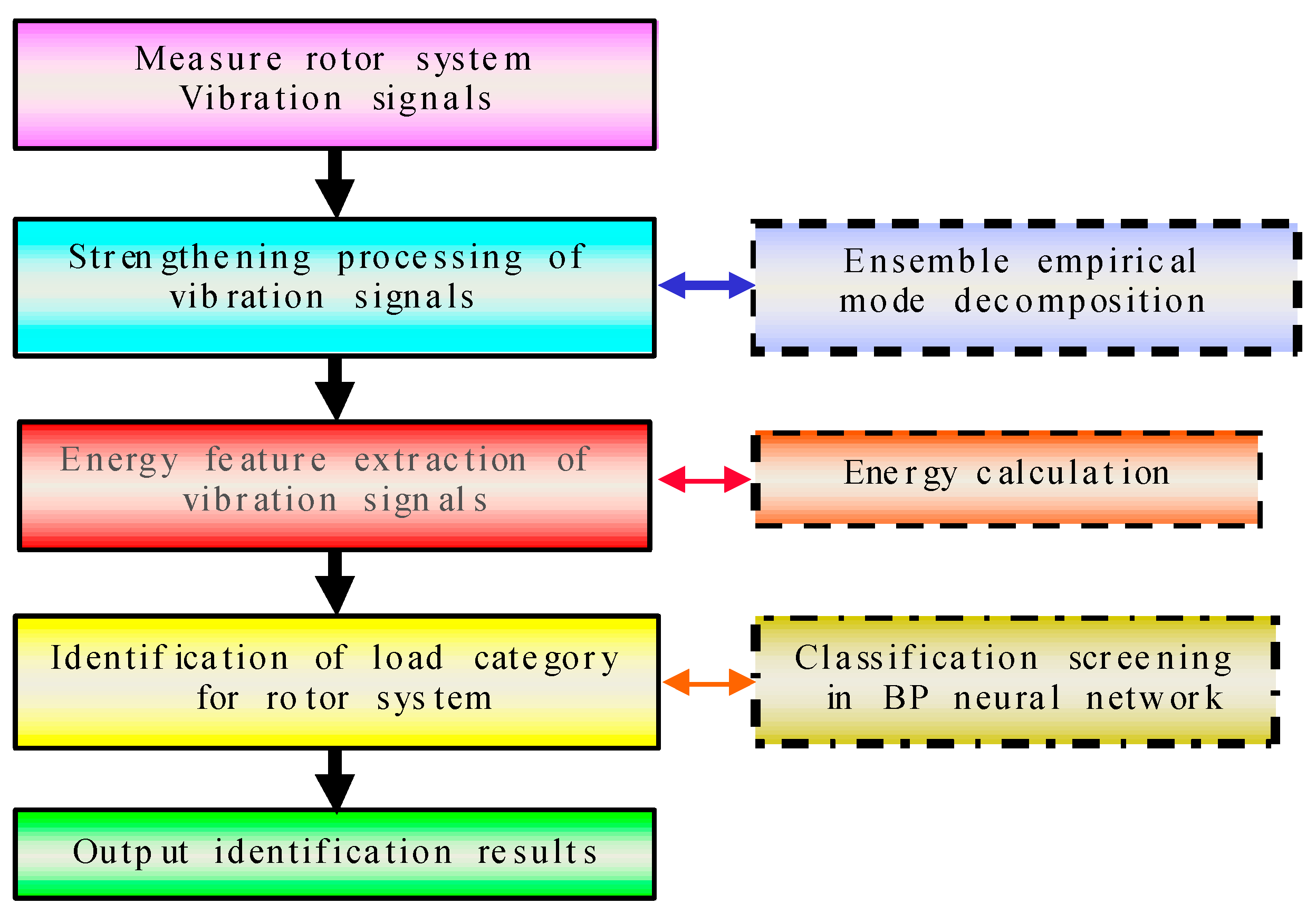
2. Methodologies of Vibration Signal Based on Load Category
2.1. Vibration Signatures Enhancement Based on EEMD
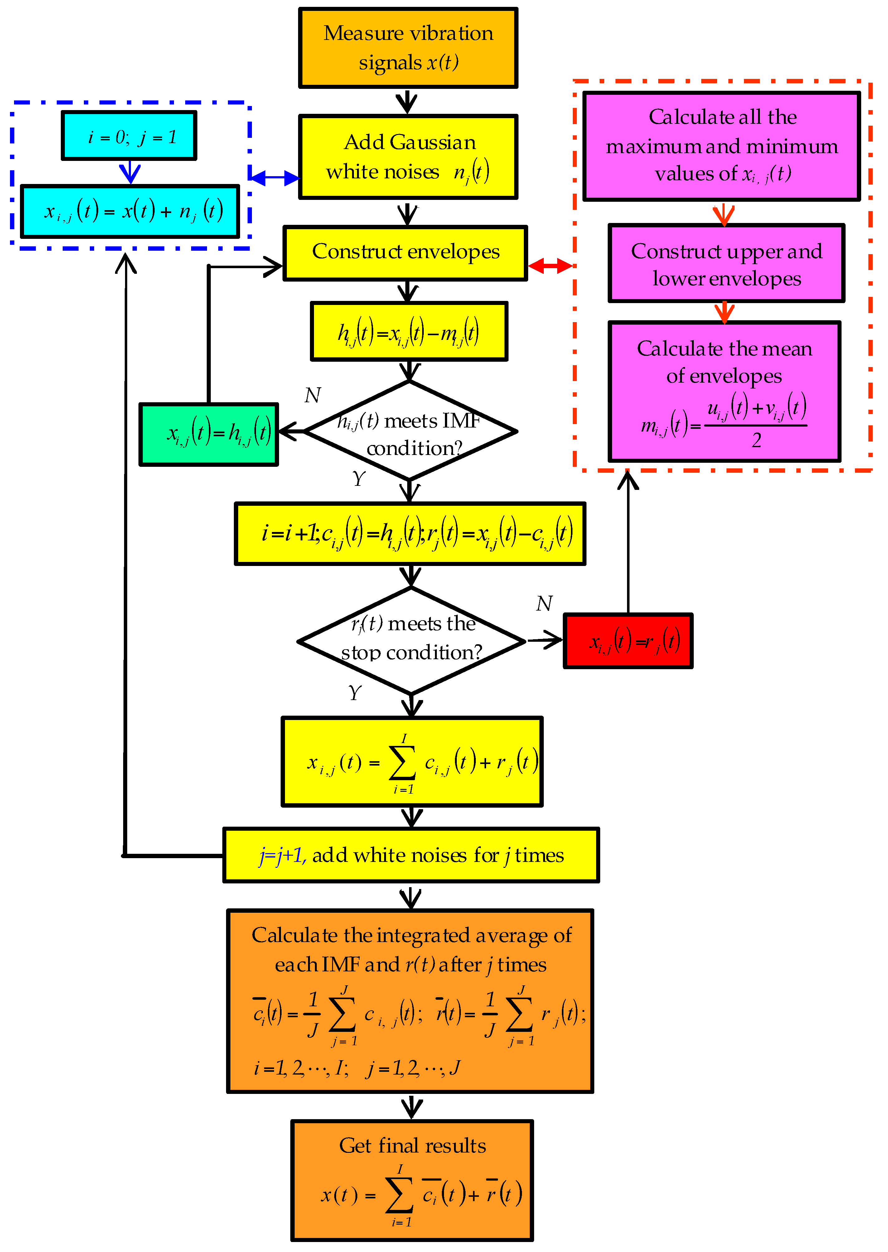
- Some Gaussian white noise sequences are added to the original signal respectively. The j-th white noise adding is taken as an example. A white noise nj(t) is added to the original signal x(t), which is expressed as:In the equation, nj(t) means adding the j-th white noise. j means the sequence of adding white noise. J denotes the total number of additions of white noise. xi,j(t) represents the i-th order signal decomposed after the j-th adding noise. i expresses the sequence of intrinsic mode function (IMF) components obtained via EMD after addition of one noise. I is the total number of IMFs.
- Then, xi,j(t) is decomposed. During this process, maximum and minimum points of the signal are calculated. Next, upper and lower envelopes of the signal are constructed, and the average mi,j(t) is calculated.In the equation, ui,j(t) and vi,j(t) mean upper and lower envelopes, respectively.
- The average signal mi,j(t) is subtracted from the original data to yield hi,j(t), a new sequence without low frequency components removed.Judging whether hi,j(t) satisfies two IMF-conditions uses the whole data sequence, and sets the number of extreme value points equal to the number of passing zero points. The maximum difference of two numbers cannot be above one point. At any point, the mean of the envelopes is zero, which is defined by the maximum and minimum local values of signals. If hi,j(t) does not meet the IMF condition, the calculation process needs to be repeated. If the criterion is met, this is the first IMF component ci,j(t). This is the highest frequency component of the signal sequence. ci,j(t) subtracted from xi,j(t) provides the new data sequence rj(t).Next, rj(t) is checked against the stop condition. Namely, when rj(t) becomes a monotone function, the screening ends. If the stop criterion is not met, rj(t) needs to be calculated again using the above-mentioned decomposition. This process is repeated until the last data sequence cannot be decomposed any further.In the formula, ci,j(t) is the i-th IMF component after EMD, when adding the j-th white noise, while rj(t) is the residual component after EMD, when adding the j-th white noise.
- Step 1. is repeated J-1 times. For each iteration, a new sequence of Gaussian white noise nj(t) is added. During EEMD, the total times of Gaussian white noise obey the statistical regularity of Equation (6).In the equation, ε is the amplitude of Gaussian white noise and εn denotes the error between the initial signal and the sum of IMFs. According to the paper [22], when J is between 100 and 300, the residual white noise error has been at a low level.
- After adding white noise for J times, for a given IMF, intrinsic mode components are calculated using integrated average processing.Meanwhile, after J times decomposition, residual components rj(t) are calculated using an integrated average processing as well.Thus, final results are obtained.In the formula, represents each IMF component, which is finally obtained after EEMD. is the final residual component.
2.2. Energy Feature Extraction of IMF Vibration Signal
- From the EEMD of the signal, select I IMF components containing information of the load.
- Solve for energy value Ei of each IMFi. Here IMFi is equal to in Equation (7).
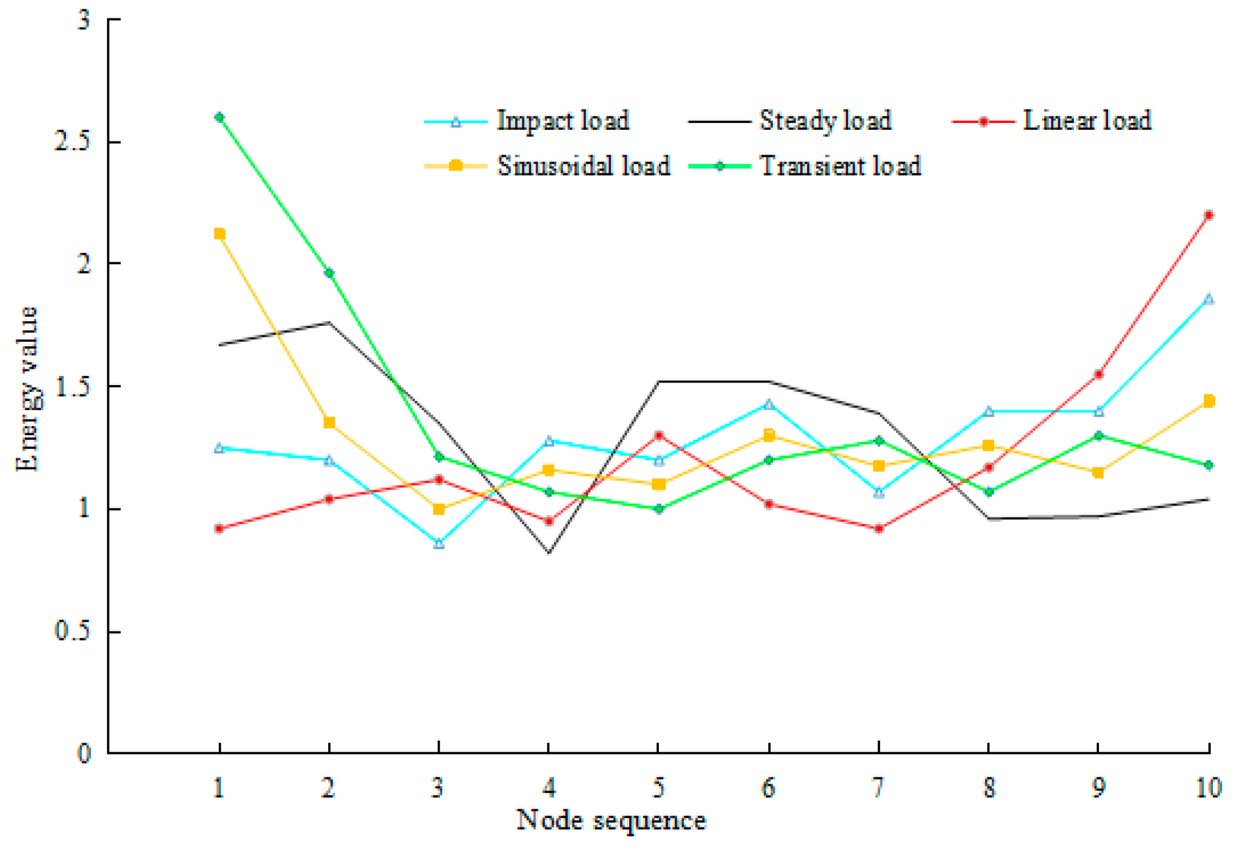
- Construct a feature vector E formed with energy.The obtained energy ratio is defined as follows:When different loads are applied to the rotor system, displacement signal energy changes in each frequency band. Energy in each frequency band contains information related to loading. Therefore, IMF energy components from the signals are extracted as feature vectors of load type.
2.3. Classification Method
2.3.1. Choice of the Classifier
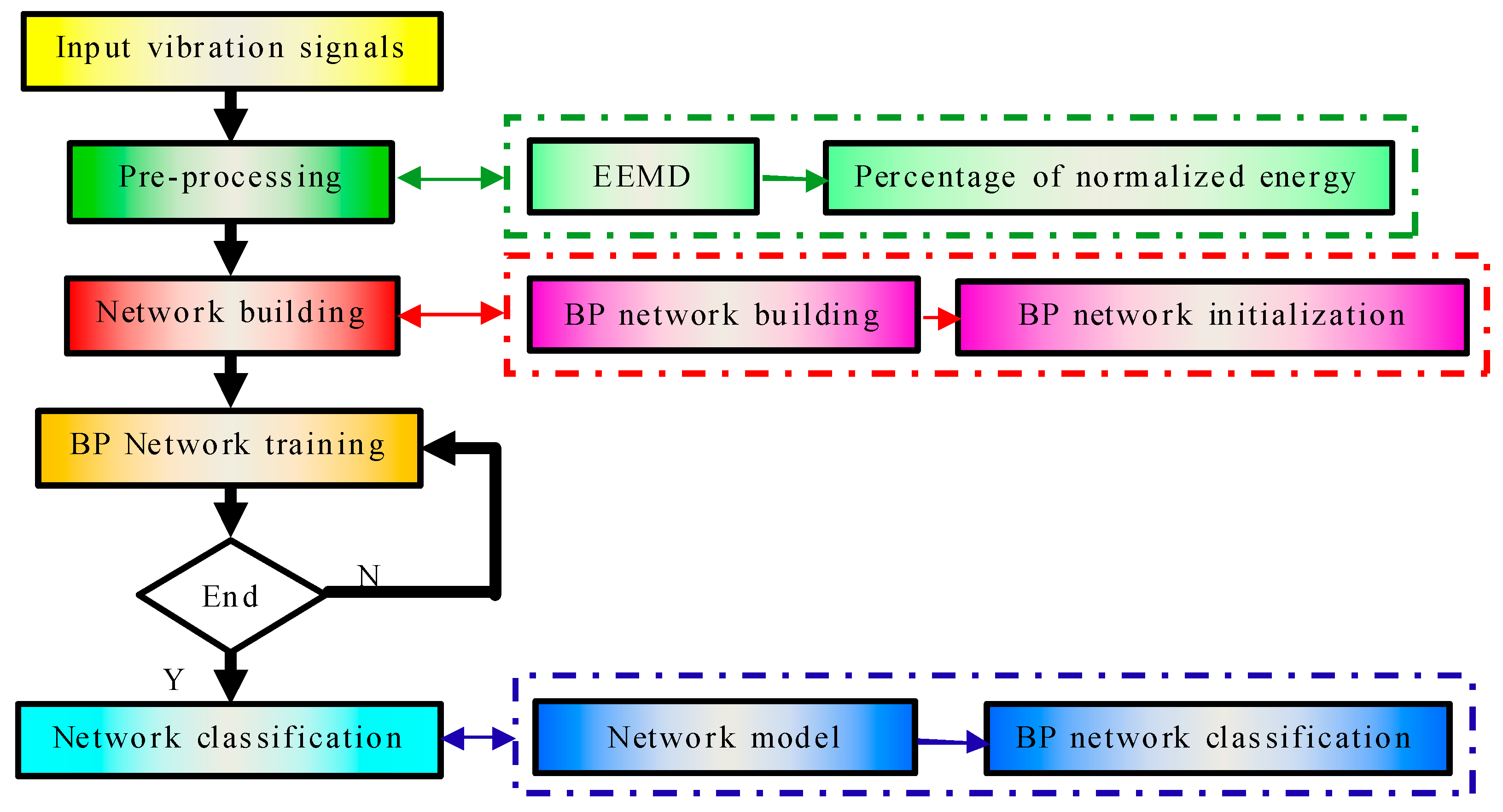
2.3.2. Classification with BP Neural Network
- Network initialization. According to input and output sequence (x, y) of the system, the network needs to determine the number of input layer nodes n, the number of hidden layer nodes l, and the number of output layer nodes m. Then, connection weights ωij and ωjk are initialized for neurons of input, hidden, and output layers. Hidden layer threshold a, and output layer threshold b are initialized. Learning rate and excitation function of neurons are specified. Number of hidden-layer nodes for the BP neural network can be designed based on empirical Equation (13). p is an adjustable integer constant between 1–10.
- Output calculation of the hidden layer. Based on input variable x, connection weights ωij between input layer and hidden layer, and hidden layer threshold a, the hidden layer yields output H.In this formula, f is the excitation function of the hidden layer. This function has a variety of forms. One of these forms has been chosen below.
- Output calculation for output layer. According to hidden layer output H, connection weight ωjk and threshold value b, BP neural network calculates the predicting output O.
- Based on the predicting output O and desired output y, prediction accuracy for the network is evaluated.
- Connection weights ωij and ωjk in the network are updated.η indicates the learning rate.
- Next, node thresholds a and b in the network are updated.
- Check if stop condition for the iterations is reached. If not, go to step 2.
3. Load Category Identification Experiments
3.1. Experimental Program
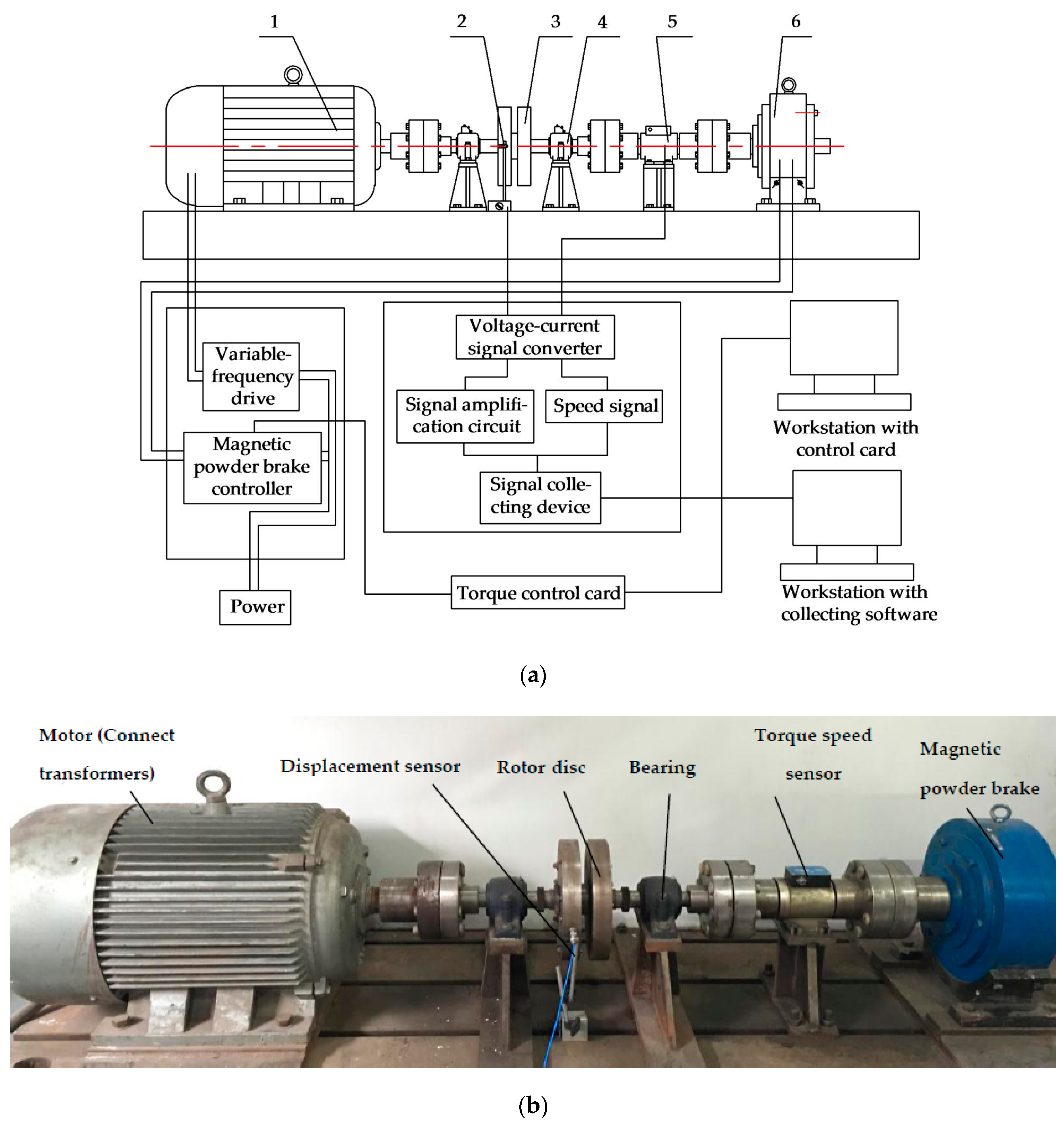
3.2. Test Platform Build
4. Analysis of Experimental Results
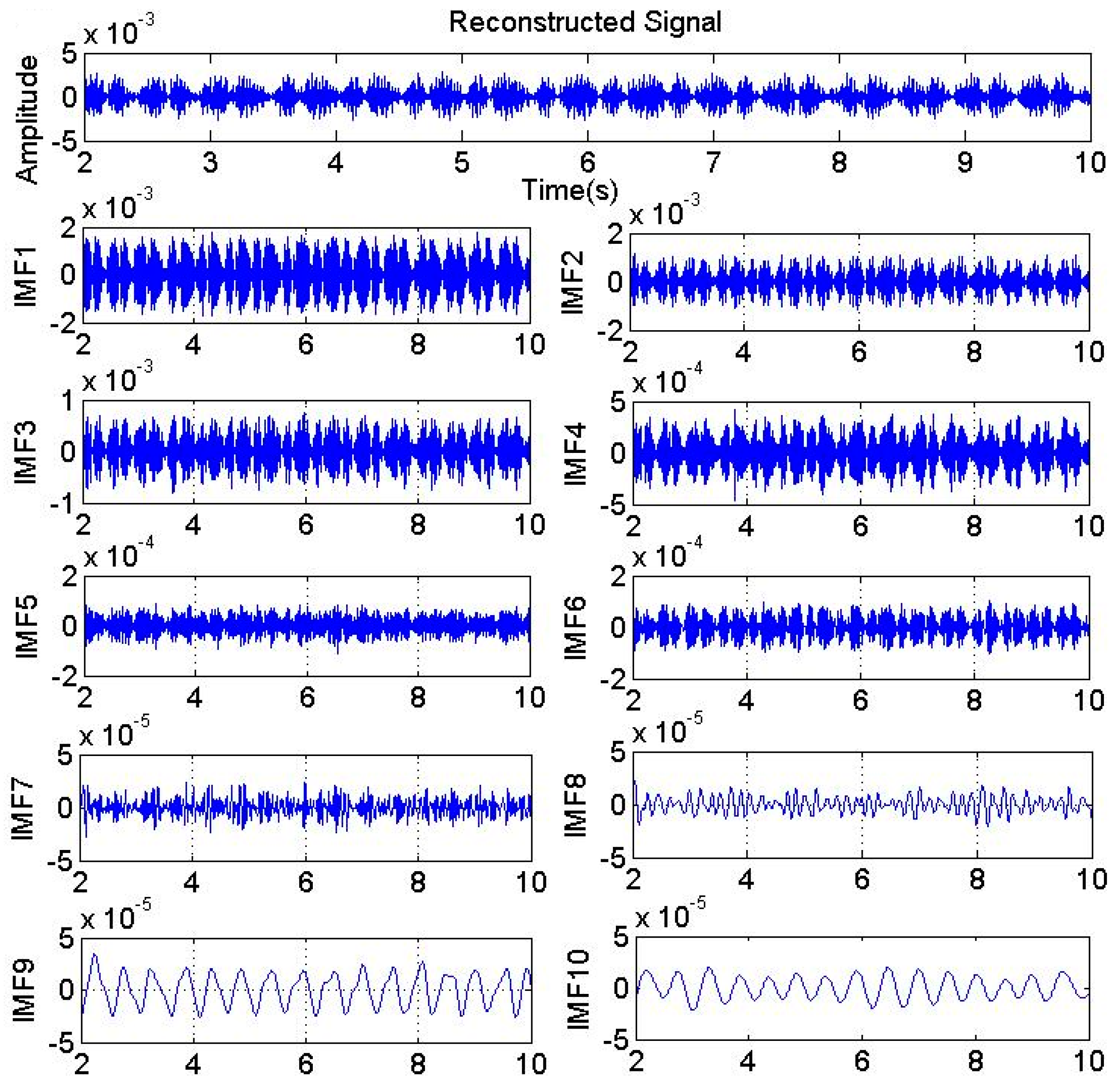
4.1. Comprehensive Pre-Processing of Load Vibration Signal
4.2. Energy Feature Extraction of Load Vibration Signal
4.3. Category Identification of Experimental Load
4.3.1. BP Neural Network Training
Number of Hidden Layer Nodes (NHLN) Setting
Node Transfer Function (NTF) Selection
Network Training Function Selection
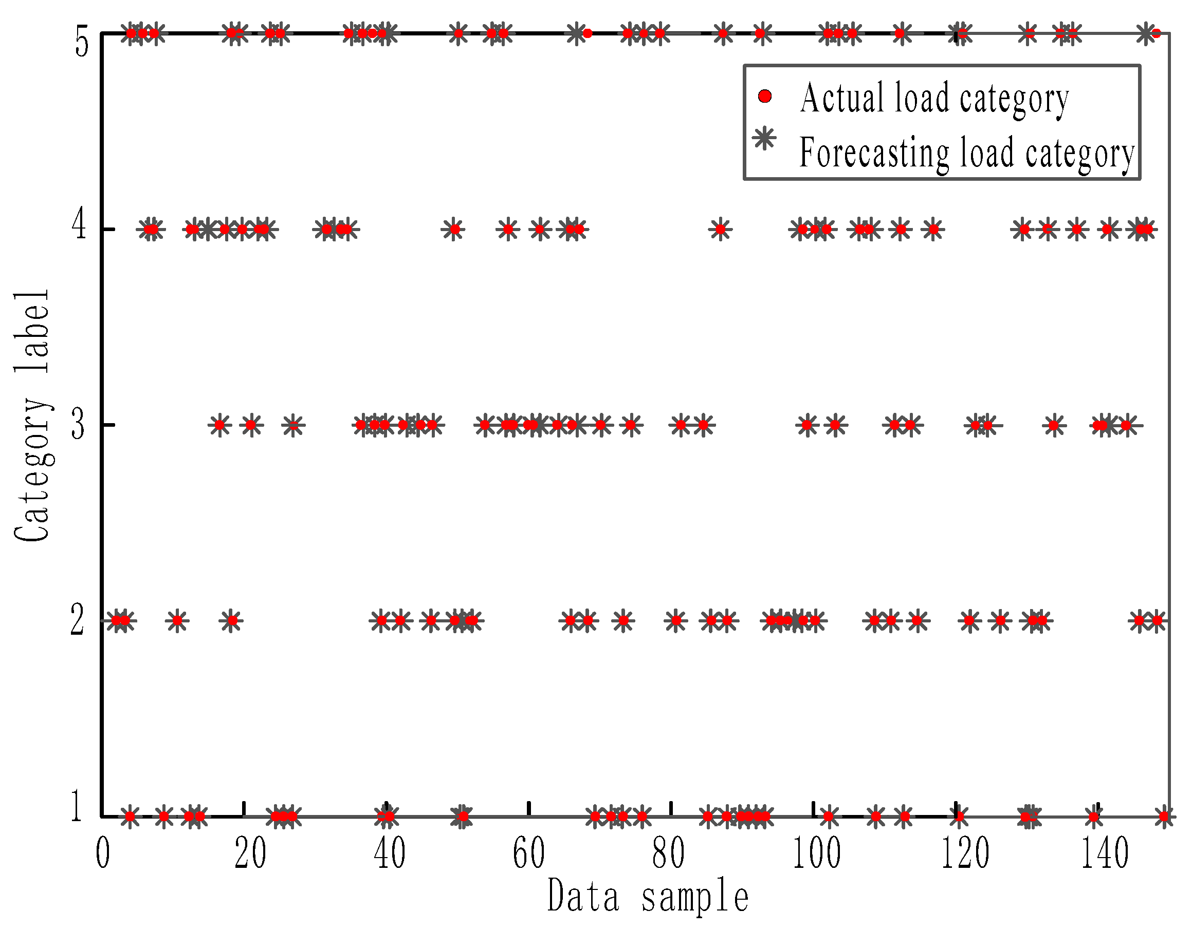
4.3.2. Load Type Identification in BP Neural Network
5. Conclusions
Acknowledgments
Author Contributions
Conflicts of Interest
References
- Hou, L.; Chen, Y.S.; Fu, Y.Q.; Li, Z.G. Nonlinear response and bifurcation analysis of a duffing type rotor model under sine maneuverload. Int. J. Non-Linear Mech. 2016, 78, 133–141. [Google Scholar] [CrossRef]
- Bessam, B.; Menacer, A.; Boumehraz, M. Detection of broken rotor bar faults in induction motor at low load using neural network. ISA Trans. 2016, 64, 241–246. [Google Scholar] [CrossRef] [PubMed]
- Husband, J.B. Developing an Efficient FEM Structural Simulation of a Fan Blade off Test in a Turbofan Jet Engine. Ph.D. Thesis, University of Saskatchewan, Saskatchewan, SK, Canada, 2007. [Google Scholar]
- Gui, C.L.; Li, Z.Y.; Sun, J. Study on dynamic behaviors of variably-loaded shaft-bearing system. Mach. Des. Res. 2005, 21, 12–16. [Google Scholar]
- Du, S.W. A new method for fault diagnosis of mine hoist based on manifold learning and genetic algorithm optimized support vector machine. Elektronika Ir Elektrotechnika 2012, 123, 99–102. [Google Scholar] [CrossRef]
- Yang, Z.C.; Jia, Y. The identification of dynamic loads. Adv. Mech. 2015, 45, 30–33. [Google Scholar]
- Fu, C.Y.; Shan, D.S.; Li, Q. Damage location identification of railway bridge based on vibration response caused by vehicles. J. Southwest Jiaotong Univ. 2011, 46, 719–725. [Google Scholar]
- Zhu, T.; Xiao, S.N.; Yang, G.W. State-of-art development of load identification and its application in study on wheel-rail forces. J. China Railw. Soc. 2011, 33, 29–36. [Google Scholar]
- Troclet, B.; Alestra, S.; Srithammavanh, V. A time domain inverse method for identification of random acoustic sources at launch vehicle lift-off. J. Vib. Acoust. Trans. ASME 2011, 133, 1–11. [Google Scholar] [CrossRef]
- Zhou, P.; Zhang, Q.; Shuai, Z.J.; Li, W.Y. Review of research and development status of dynamic load identification in time domain. Noise Vib. Control 2014, 34, 6–11. [Google Scholar]
- Ryerkerk, M.L.; Averill, R.C.; Deb, K.; Goodman, E.D. Solving metameric variable-length optimization problems using genetic algorithms. Genet. Program. Evolvale Mach. 2017, 18, 247–277. [Google Scholar] [CrossRef]
- Lin, J.H.; Guo, X.L.; Zhi, H.; Howsonb, W.P.; Williams, F.W. Computer simulation of structural random loading identification. Comput. Struct. 2001, 79, 375–387. [Google Scholar] [CrossRef]
- Wang, X.M. Neural Network Introduction; Science Press: Beijing, China, 2017. [Google Scholar]
- Yu, D.L.; Deng, S.C.; Zhang, Y.M.; Qi, W.G. Working condition diagnosis method based on SVM of submersible plunger pump. Trans. China Electrotech. Soc. 2013, 28, 248–254. [Google Scholar]
- Zhang, Z.F.; Fu, J.P.; Miao, J.S.; Zhao, Z.J. Research on the fault diagnosis technology of the water-projectile test posterior to the gun repair. J. Gun Launch Control 2017, 38, 95–100. [Google Scholar]
- Li, B.; Chow, M.Y.; Tipsuwan, Y.; Hung, J.C. Neural-network-based motor rolling bearing fault diagnosis. IEEE Trans. Ind. Electron. 2000, 47, 1060–1069. [Google Scholar] [CrossRef]
- Sawalhi, N.; Randall, R.B. The Application of Spectral Kurtosis to Bearing Diagnaosis. In Proceedings of the Acoustics, Gold Coast, Australia, 3–5 November 2004; pp. 393–398. [Google Scholar]
- Su, W.S.; Wang, F.T.; Zhu, H.; Guo, Z.G.; Zhang, Z.X.; Zhang, H.Y. Feature extraction of rolling element bearing fault using wavelet packet sample entropy. J. Vib. Meas. Diagn. 2011, 312, 162–166. [Google Scholar]
- Fang, Y.R.; Shen, H.F.; Qiu, K.N. The new method of Rayleigh wave signal purification based on EMD. Earthq. Eng. Eng. Dyn. 2017, 37, 6–71. [Google Scholar]
- Zhang, M.L.; Wang, T.Z.; Tang, T.H. An imbalance fault detection method based on data normalization and EMD for marine current turbines. ISA Trans. 2017, 68, 302–312. [Google Scholar] [CrossRef] [PubMed]
- Huang, N.E.; Wu, Z.H. Ensemble empirical mode decomposition: A noise assisted data analysis method. Adv. Adapt. Data Anal. 2009, 1, 1–41. [Google Scholar]
- Mo, J.L.; He, Q.; Hu, W.P. An Adaptive Thresh-Old De-Noising Method Based on EEMD. In Proceedings of the 2014 IEEE International Conference on Signal Processing, Communi-Cations and Computing (ICSPCC), Hangzhou, China, 26–30 October 2014; pp. 209–214. [Google Scholar]
- Shao, Y.M.; Liang, J.; Gu, F.S.; Chen, Z.G.; Ball, A. Fault Prognosis and Diagnosis of An Automotive Rear Axle Gear Using a RBF-BP Neural Network. In Proceedings of the 9th International Conference on Damage Assessment of Structures (DAMAS), Oxford, UK, 11–13 July 2011; pp. 11–13. [Google Scholar]
- Zhao, L.F.; Zhou, C.G.; Zhong, J.C. Fault diagnosis based on EMD and neural networks. J. Ocean Univ. China 2004, 34, 298–300. [Google Scholar]
- Zhao, G.; Wang, H.; Liu, G.; Wang, Z.Q. Optimization of stripping voltammetric sensor by a back propagation artificial neural network for the accurate determination of Pb(II) in the presence of Cd(II). Sensors 2016, 16, 3. [Google Scholar] [CrossRef] [PubMed]


| Classifier | Time (s) | Accuracy (%) |
|---|---|---|
| SVM | 2.215 | 92.071 |
| RBFNN | 0.633 | 83.182 |
| BPNN | 3.218 | 94.550 |
| Load Type | Expression (Nm) | |||
| impact (0.5 s) | M = 40 | M = 50 | M = 55 | M = 60 |
| steady | M = 40 | M = 50 | M = 55 | M = 60 |
| linear | M = 0.1 t + 40 | M = 0.1 t + 50 | M = 0.2 t + 40 | M = 0.2 t + 50 |
| sinusoidal | M = sin4πt + 40 | M = sin4πt + 60 | M = sin10πt + 40 | M = 10 sin4πt + 40 |
| transient (3 s) | M = 40 | M = 50 | M = 55 | M = 60 |
| Load Type | Expression (Nm) | |||
| impact (0.5 s) | M = 65 | M = 70 | M = 75 | M = 80 |
| steady | M = 65 | M = 70 | M = 75 | M = 80 |
| linear | M = 0.5 t + 50 | M = t + 30 | M = t + 40 | M = t + 50 |
| sinusoidal | M = 10 sin4πt + 60 | M = 10 sin10πt + 40 | M = 20 sin4πt + 60 | M = 20 sin10πt + 60 |
| transient (3 s) | M = 65 | M = 70 | M = 75 | M = 80 |
| Number of Nodes | 5 | 6 | 7 | 8 | 9 |
| Error (10−9) | 9.996 | 9.961 | 7.705 | 9.962 | 9.571 |
| training times | 990 | 972 | 508 | 290 | 292 |
| Number of Nodes | 10 | 11 | 12 | 13 | 14 |
| Error (10−9) | 1.297 × 10⁻² | 2.511 × 10⁻¹ | 4.463 × 10⁻³ | 2.526 | 8.881 × 10⁻¹ |
| training times | 156 | 72 | 77 | 90 | 86 |
| Load Type | Impact | Steady | Linear | Sinusoidal | Transient |
|---|---|---|---|---|---|
| sorting code | 1 | 2 | 3 | 4 | 5 |
| expected output | [1 0 0 0 0] | [0 1 0 0 0] | [0 0 1 0 0] | [0 0 0 1 0] | [0 0 0 0 1] |
| Type | T1 | T2 | T3 | T4 | T5 |
| impact (0.5 s) | 0.0965 | 0.0927 | 0.0664 | 0.0988 | 0.0927 |
| steady | 0.1285 | 0.1354 | 0.1038 | 0.0631 | 0.1170 |
| linear | 0.0755 | 0.0853 | 0.0919 | 0.0779 | 0.1066 |
| sinusoidal | 0.1624 | 0.1034 | 0.0766 | 0.0889 | 0.0843 |
| transient (3 s) | 0.1874 | 0.1415 | 0.0875 | 0.0771 | 0.0721 |
| Type | T6 | T7 | T8 | T9 | T10 |
| impact (0.5 s) | 0.1104 | 0.0826 | 0.1082 | 0.1081 | 0.1436 |
| steady | 0.1169 | 0.1069 | 0.0738 | 0.0746 | 0.0800 |
| linear | 0.0837 | 0.0755 | 0.096 | 0.1271 | 0.1805 |
| sinusoidal | 0.0996 | 0.0900 | 0.0965 | 0.0881 | 0.1102 |
| transient (3 s) | 0.0865 | 0.0922 | 0.0771 | 0.0937 | 0.0849 |
| No. | T1 | T2 | T3 | T4 | T5 |
| 1 | 0.1336 | 0.1044 | 0.0903 | 0.1100 | 0.0965 |
| 2 | 0.7920 | 0.0785 | 0.0164 | 0.0032 | 0.0050 |
| 3 | 0.0924 | 0.0970 | 0.1131 | 0.0863 | 0.1096 |
| No. | T6 | T7 | T8 | T9 | T10 |
| 1 | 0.1150 | 0.0954 | 0.0878 | 0.0788 | 0.0882 |
| 2 | 0.0048 | 0.0111 | 0.0190 | 0.0382 | 0.0318 |
| 3 | 0.0999 | 0.0917 | 0.1066 | 0.0897 | 0.1137 |
© 2017 by the authors. Licensee MDPI, Basel, Switzerland. This article is an open access article distributed under the terms and conditions of the Creative Commons Attribution (CC BY) license (http://creativecommons.org/licenses/by/4.0/).
Share and Cite
Zhang, K.; Yang, Z. Identification of Load Categories in Rotor System Based on Vibration Analysis. Sensors 2017, 17, 1676. https://doi.org/10.3390/s17071676
Zhang K, Yang Z. Identification of Load Categories in Rotor System Based on Vibration Analysis. Sensors. 2017; 17(7):1676. https://doi.org/10.3390/s17071676
Chicago/Turabian StyleZhang, Kun, and Zhaojian Yang. 2017. "Identification of Load Categories in Rotor System Based on Vibration Analysis" Sensors 17, no. 7: 1676. https://doi.org/10.3390/s17071676
APA StyleZhang, K., & Yang, Z. (2017). Identification of Load Categories in Rotor System Based on Vibration Analysis. Sensors, 17(7), 1676. https://doi.org/10.3390/s17071676