1. Introduction
The Internet of Things (IoT) aims to provide connectivity among a huge number of “things” anytime and anywhere. This will highly impact every aspect of the world we live in, including economics, politics, and social life. Emerging IoT applications and services, such as smart meters, environmental/agricultural monitoring and automation of industrial processes, require myriads of battery-powered smart things (e.g., sensors, actuators, controllers) connected together in an energy efficient way. Currently, there are two categories of low-power IoT communication technologies: wireless personal area network (WPAN) and low-power wide area network (LPWAN) technologies. Within short transmission range (i.e., tens of meters), WPAN technologies (e.g., Bluetooth Low Energy, ZigBee) provide relatively high throughput (i.e., up to a few hundred kilobits per second), while long-range communications (i.e., up to several kilometers) can be supported by LPWAN technologies (e.g., LoRA, SigFox) at much lower throughput (i.e., up to at most a few kilobits per second). As the transmission range of the WPAN technologies is too short and throughput of the LPWAN technologies is too low, both of them can only be applied in a limited set of IoT scenarios. Therefore, a gap still exists for a low-power IoT communication technology that offers sufficient throughput over longer ranges.
The recently released IEEE 802.11ah Wi-Fi standard, marketed as Wi-Fi HaLow, fills this gap. It operates in the unlicensed sub-1 GHz frequency bands (e.g., 863–868 MHz in Europe, 755–787 MHz in China and 902–928 MHz in North-America). Similar to previous Wi-Fi standards, it supports several modulation and coding schemes (MCS) in order to offer a trade-off between throughput, range and energy efficiency. This allows it to support transmission ranges from 100 m up to 1 km with data rates between 0.15 Mbps and 346.67 Mbps. Thus, IEEE 802.11ah has the potential to achieve much higher transmission ranges than existing WPAN and much higher throughput than both WPAN and LPWAN technologies. On the MAC (Media Access Control) layer, in order to increase efficiency in the face of a large number of densely deployed, energy constrained stations, several innovative mechanisms are introduced, including hierarchical organization, short MAC header, restricted access window (RAW), traffic indication map (TIM) segmentation and target wake time (TWT).
The RAW feature aims to increase scalability in dense IoT networks, where a large number of stations connect to a single access point (AP). With RAW, stations are divided into groups, limiting simultaneous channel access to one group. Therefore, the collision probability for upstream traffic is highly reduced. However, the grouping strategy, which decides how to split stations among groups, is not mentioned in the standard. Concretely, a station grouping algorithm should be implemented at the AP side to determine the number of RAW groups, the duration of each group, and how to divide stations among them. Furthermore, these parameters should be dynamically adapted by the AP between consecutive beacon intervals. In previous work, we conducted an in-depth analysis of the influence of network and traffic conditions on the optimal station grouping parameters [
1]. We concluded that the optimal parameters depend on a wide range of network variables, such as number of stations, network load and traffic patterns. This shows the need for dynamic station grouping algorithms that determine the optimal station grouping parameters based on the current network and traffic conditions. As these conditions change, the algorithm should similarly adapt.
In this article, we present a novel real-time station grouping algorithm that adapts the RAW parameters based on the current (estimated) traffic conditions, optimized for sensor networks with mainly upstream traffic. It improves upon the state of the art in three ways. First, it is designed for dynamic and heterogeneous traffic conditions, where each station has a different packet transmission interval that may change over time. Second, it only uses information readily available on the AP side, estimating station-side variables based on available data. Third, it can be executed in real time, not relying on at-runtime evaluation of complex mathematical models. The combination of these three factors allows the algorithm to be deployed in realistic environments, executing it at the start of each beacon interval for instantaneous adaptation to changes in traffic conditions. To the best of our knowledge, this is the first real-time IEEE 802.11ah station grouping algorithm that can cope with dynamic and heterogeneous traffic. The algorithm is thoroughly evaluated using our previously presented 802.11ah ns-3 simulator [
2].
The remainder of this article is structured as follows.
Section 2 introduces related research on IEEE 802.11ah station grouping.
Section 3 provides a brief overview of the IEEE 802.11ah RAW feature. The real-time station grouping algorithm for dynamic traffic is presented in
Section 4.
Section 5 describes the derivation of the optimal value of two input parameters used by the proposed algorithm. In
Section 6, we provide a comparison of the algorithm to enhanced distributed channel access/distributed coordination function (EDCA/DCF) and static grouping using simulation results. Finally, conclusions and future work are discussed in
Section 7.
2. Related Work
Even though the IEEE 802.11ah standard was only officially published recently, research on IEEE 802.11ah has been conducted for several years. Several articles [
3,
4,
5,
6,
7,
8] provide a deep overview of the key features of the new technology, fully describing the advantages and challenges in the design of PHY and MAC layer schemes. Moreover, performance assessment on IEEE 802.11ah in four common machine-to-machine (M2M) scenarios, i.e., smart metering, agriculture monitoring, animal monitoring, and industrial automation, has been conducted by Adame et al. [
5]. Baños et al. [
8] thoroughly evaluated performance of IEEE 802.11ah in comparison to the most notable IEEE 802.11 standards, and exposed the capabilities of IEEE 802.11ah in supporting different IoT applications.
Several recent works study physical layer aspects of 802.11ah and sub-1 GHz communications [
9,
10,
11,
12,
13,
14]. Hazmi [
9] conducts assessment on the link budget, and derives the achievable data rate and optimal packet size of 802.11ah. Aust and Ito [
10] study three urban propagation path loss models of 802.11ah for carrier frequencies at 900 MHz. Li and Wang [
14] compare the indoor coverage and time delay performance between IEEE 802.11g and IEEE 802.11ah in M2M communications. Aust and Prasad [
12] proposed an IEEE 802.11ah prototype that is configured as a self-contained M2M wireless sensor system and allows an over-the-air protocol performance assessment. Casas and Papaparaskeva [
13] introduced a design for a programmable 802.11ah station based on the Cadence-Tensilica Fusion digital signal processor (DSP). Aust, Prasad and Niemegeers [
11] built a real-time Multiple-input, multiple-output orthogonal frequency-division multiplexing (MIMO-OFDM) testing platform for evaluating narrow-band sub-1GHz transmission characteristics. Moreover, Ba et al. [
15] developed an 802.11ah fully-digital polar transmitter, this hardware prototype passes all the PHY requirements of the mandatory modes in IEEE 802.11ah with 4.4% error-vector-magnitude (EVM), while consuming only 7.1 mW with 0 dBm output power.
More relevant to the research presented in this article is work focusing on RAW analysis and optimization. Several studies have been conducted on the optimality of RAW configurations given specific network and traffic conditions [
1,
16,
17]. Park [
16] showed the effectiveness of RAW to mitigate the hidden node problem. Zhao et al. [
17] evaluated RAW in terms of energy efficiency, showing that increasing the number of RAW groups significantly improves energy efficiency for sensor stations. Finally, in our own previous work [
1], we evaluated the optimal RAW station grouping configuration under a variety of traffic conditions, proving the need for a dynamic regrouping algorithm, that takes into account changes in network and traffic conditions.
Several such station grouping algorithms have been proposed in literature, as shown in
Table 1. The goal of these algorithms is to determine RAW parameters (i.e., number of groups and slots, group duration, and station partitioning among groups), given the current network conditions (e.g., number of stations, traffic demand, station location). For each algorithm,
Table 1 shows the assumed upstream traffic conditions, the optimization objective, and the used algorithmic method. The surveyed algorithms focus on upstream traffic, as station grouping mainly improves upstream scalability, and it is the main type of traffic in sensor networks. The traffic conditions consist of two parts. First, the traffic intensity can be categorized as either (i) one packet per station per slot; (ii) saturated traffic for each station; (iii) a static finite number of packets per station per slot and (iv) a dynamic (i.e., changing from slot to slot) finite number of packets per station per slot. Second, the inter-station traffic differentiation is either homogeneous (i.e., all stations have the same traffic intensity) or heterogeneous (i.e., different stations may have different traffic intensities). The considered objectives are contention minimization (i.e., through hidden node mitigation), throughput maximization, energy consumption minimization, or a combination. It is clear that, to be applicable to real scenarios, supported traffic conditions should be both dynamic and heterogeneous.
The algorithms presented in the table are broadly based on two approaches: (i) analytical modeling and (ii) set partitioning. The analytical models make use of different techniques, such as probability theory [
22,
27,
28], Markov chains [
23,
29,
30], multi-objective game theory [
25], and maximum likelihood estimation [
26]. They all aim to optimize throughput, energy consumption, or a combination of both. Generally, they are computationally hard. This makes it infeasible to execute them in real time on actual AP hardware, where, at most, a few milliseconds are available at the start of the beacon interval to calculate a new RAW configuration. Moreover, such models require information about the station’s traffic demand that is not readily available on the AP side. To simplify the modeling process, all existing models for RAW focus on homogeneous traffic with either one packet per station or under saturation. The combination of these factors make such models useful only from a theoretical point of view, in order to analyze the effectiveness of RAW under a variety of conditions. However, they cannot be used for real-time station grouping under dynamic and realistic traffic conditions.
The set partitioning algorithms are much simpler. They assume the number of RAW slots and groups is given, and decide how to partition the associated stations among them, according to some metric. Their simplicity makes it computationally feasible to deploy them in real networks. Older work assumes simplified saturated and homogeneous network conditions. Moreover, it focuses on simple partitioning metrics, such as fully random [
31] or based on the back-off timer value [
24], which, in reality, is not known to the AP. Recently, some more interesting approaches have popped up. Several algorithms focus on mitigating hidden node collisions by splitting mutually hidden nodes into orthogonal groups [
18,
19,
20]. Additionally, Chang et al. proposed a set partitioning algorithm that assumes the (static) traffic demand of each station is known by the AP and load balances them across groups [
21]. Most of these recent algorithms still assume simplified homogeneous traffic [
18,
20]. However, two algorithms [
19,
21] focus on more realistic traffic, where stations have heterogeneous, static and non-saturated traffic.
Although the algorithms of Dong [
19] and Chang [
21] take a step in the right direction by supporting more realistic traffic and real-time execution, they still have several shortcomings that we aim to address in this article. First, none of the presented algorithms take into account traffic dynamics. In a real network, the upstream traffic intensity of stations may change over time for a variety of reasons, and the algorithm should therefore adapt to these changes. Second, they expect all information, such as the exact traffic intensity of each station, to be readily available on the AP side, which, in reality, is not the case. Third, they assume that the number of groups and slots as well as their duration are given, and only the partitioning of stations among them needs to be solved. The number of groups and their duration, however, significantly influence RAW optimality [
1]. All parameters should therefore be jointly optimized.
In this paper, we present a station grouping algorithm for the IEEE 802.11ah RAW mechanism that addresses these shortcomings. It supports both dynamic and heterogeneous traffic, real-time execution, estimation of station traffic intensity on the AP side , and optimization of all RAW parameters (i.e., number of groups and slots, group duration, and station partitioning). Last but not least, it is evaluated using our IEEE 802.11ah ns-3 packet-based network simulator [
2], which exhibits realistic propagation behavior (e.g., channel errors, capture effect). These propagation effects are often ignored, but significantly affect performance results.
3. IEEE 802.11ah Restricted Access Window
IEEE 802.11ah operates over a set of unlicensed radio bands (all in the sub-1 GHz spectrum), supporting up to 1 km transmission range, and allowing up to 8192 stations to associate with a single AP. Due to these features, 802.11ah is a highly attractive wireless communication technology for long-distance IoT use cases, such as smart meters and environmental/agricultural monitoring. This section provides an overview of the RAW station grouping feature of the 802.11ah standard, which is the focus of this article. More detailed overview of the complete standard can be found in existing literature [
4,
5,
6,
7].
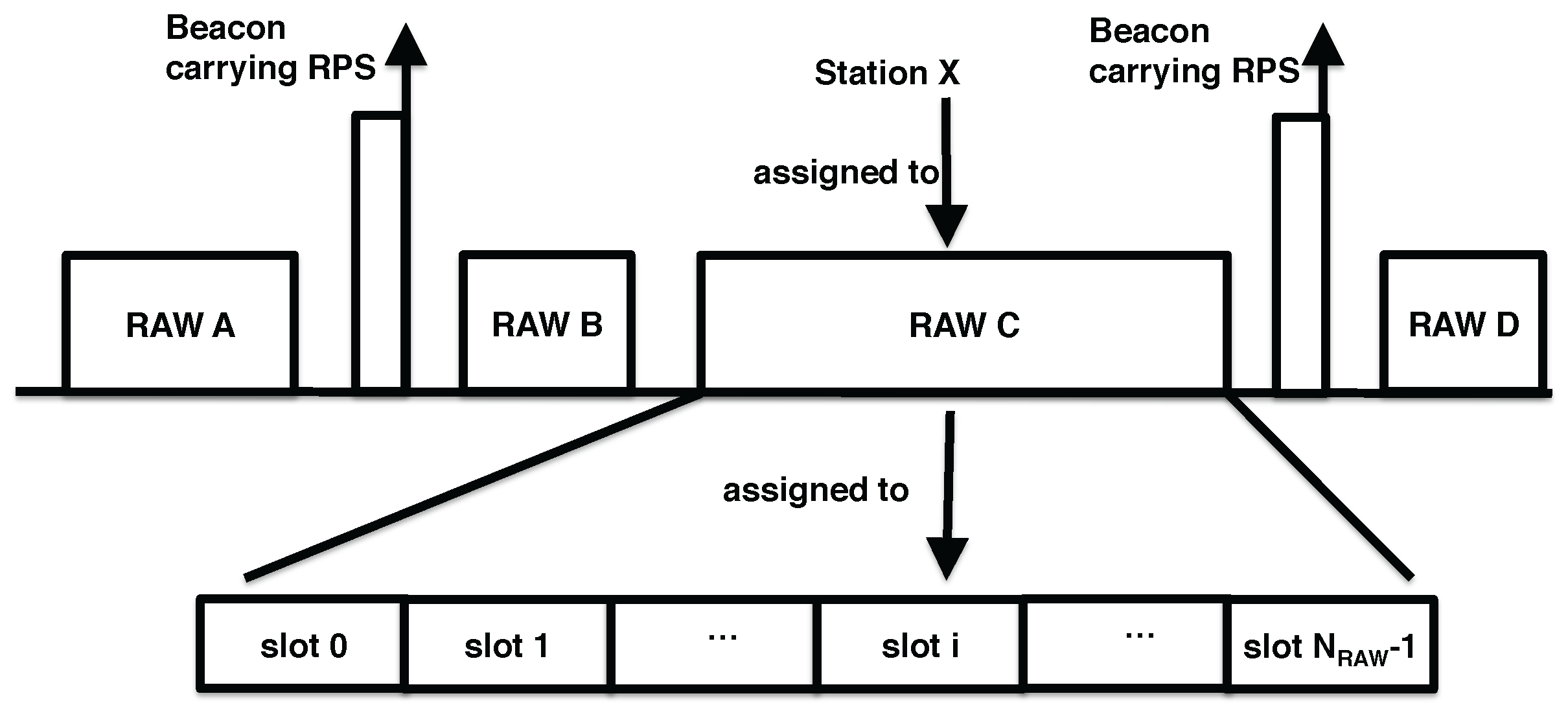
The goal of the RAW mechanism is to mitigate collisions and improve performance in dense IoT networks where a large number of stations are contending for channel access simultaneously. It splits stations into groups and only allows stations assigned to a certain group to access the channel at specific times.
Figure 1 schematically depicts how RAW works. Specifically, the channel time is split into several intervals, some of which are assigned to RAW groups, while the others are considered as shared channel airtime and can be accessed by all stations. Each interval assigned to a RAW group is preceded by a beacon frame carrying a RAW parameter set (RPS) information element that specifies the RAW related information, such as the stations belonging to the group, as well as the group start time. Moreover, each RAW group consists of one or more slots, over which the stations assigned to the RAW group are evenly split (using round robin assignment). The RPS information element also contains the number of slots, slot format and slot duration count sub-fields, which jointly determine the RAW slot duration as follows [
32]:
where
C represents
slot duration count sub-field, which is either
or
bits long if the slot format sub-field is set to respectively 1 or 0. The
number of slots field is
bits long. When
, each RAW consists of at most eight slots and the maximum value of
C is
, the slot duration is up to
ms. Otherwise, each RAW consists of at most 64 slots and the maximum value of
C is
, the slot duration is limited to 31.1 ms. Stations are mapped to slots as follows [
32]:
where
is the index of
RAW slot to which the station is mapped.
is the number of slots in one RAW.
is the offset value in the mapping function to improve fairness and equals the two least significant octets of the
FCS field of the S1G beacon frame, and
x is the index of the station.
Figure 1 shows an example of the RAW slot assignment procedure.
The RPS also contains the cross slot boundary (CSB) sub-field. Stations are allowed to continue their ongoing transmissions even after the end of the current RAW slot when CSB is set to true. Otherwise, stations should not start a transmission if the remaining time in the current RAW slot is not enough to complete it.
Different from previous IEEE 802.11 standards, each station uses two back-off states of enhanced distributed channel access (EDCA) to manage transmission inside and outside their assigned RAW slot respectively (cf.
Figure 2). The first back-off function state is used outside RAW slots, while the second is used inside. For the first back-off state, the station suspends its back-off timer at the start of each RAW, and restores and resumes the back-off timer at the end of the RAW. For the second back-off state, stations start back-off with initial back-off state inside their own RAW slot, and discard the back-off state at the end of their RAW slot, effectively restarting their back-off at the start of their next RAW period. As shown in
Figure 2, station 1 is inside the RAW group and assigned to slot 1, while station 2 is not included in this RAW group. Therefore, station 1 uses the first back-off state outside its RAW slot period and the second back-off state inside its RAW slot, while station 2 only uses the first back-off state outside the RAW group period and goes into a sleep state inside the RAW group period.
4. Real-Time RAW Parameter Optimization
This section introduces the RAW optimization problem addressed in this article, and subsequently proposes the Traffic-Adaptive RAW Optimization Algorithm (TAROA). TAROA solves the RAW optimization problem in real-time, and is able to instantaneously adapt to changes in station association and traffic demand.
Table 2 provides an overview of the variables used in the description of the RAW optimization problem and TAROA.
4.1. Problem Statement
We consider IoT sensor-based monitoring scenarios, where a large set of sensors send measurements to a back-end server (through the AP) at specific time intervals. A sensor , also referred to as a station, has a packet transmission interval , which may change over time (e.g., when an environmental event triggers a change in the sensor measurement interval).
The goal of RAW optimization is to assign stations to a set of RAW slots
during each beacon interval
b, maximizing the number of successful transmissions. As an input, it uses only information readily available at the access point. The first input is the last-in-first-out (LIFO) queue of times a packet was successfully received by the AP from station
s or
, where
represents the time of the last successful packet reception. The second input is the LIFO queue of transmission results (i.e., success or failure)
, where
is the result of the last transmission. A packet transmission is considered a failure if a RAW slot was assigned to a station, but no packet was received during that slot. The output of RAW optimization is, for each beacon interval
b, the set of RAW slots
, the set of stations
assigned to each slot
r, and the duration
of each slot
r. The goal can then be formally defined as:
where
represents the number of packets successfully received by the AP from station
s during beacon interval
b.
4.2. Traffic-Adaptive RAW Optimization Algorithm (TAROA) Overview
TAROA aims to solve the aforementioned problem by estimating the transmission interval of each station s on the AP side (as it is not known by the AP). This estimate is used to determine for each beacon interval b the set of RAW groups and slots , their duration , and the stations assigned to each of them .
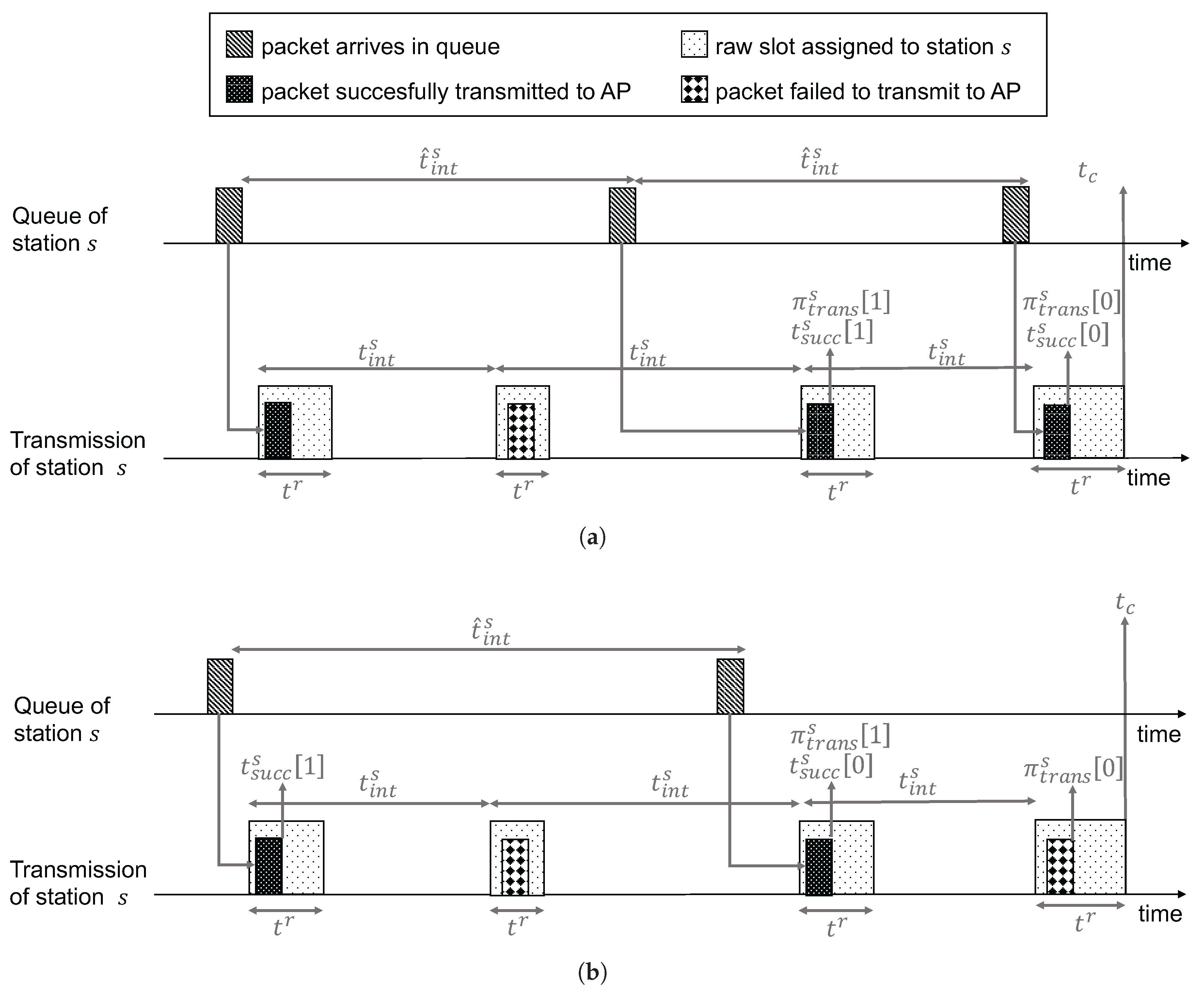
Figure 3 depicts an example time line up to the current time
for a single station attempting to transmit several packets. Station
s places a packet in its transmit queue every
seconds, while the access point estimates the related transmission interval as
. The closer this estimate is to the real value, the lower the transmission latency will be for station
s. Based on this estimate, the AP assigns RAW slots of varying duration
to
s. At the top,
Figure 3a depicts an example where the last transmission attempt at time
is successful. At the bottom,
Figure 3b shows a related example where the last transmission attempt fails, due to a lack of packets in the queue of station
s. For both cases, the figures graphically depict the parameter values for the last two transmissions results (i.e.,
and
) and the last two successful transmission times (i.e.,
and
). These values are used by the transmission interval estimation algorithm (i.e., Algorithm 1) to calculate
at the start of each beacon interval.
| Algorithm 1: Estimate transmission interval of station |
![Sensors 17 01559 i001]() |
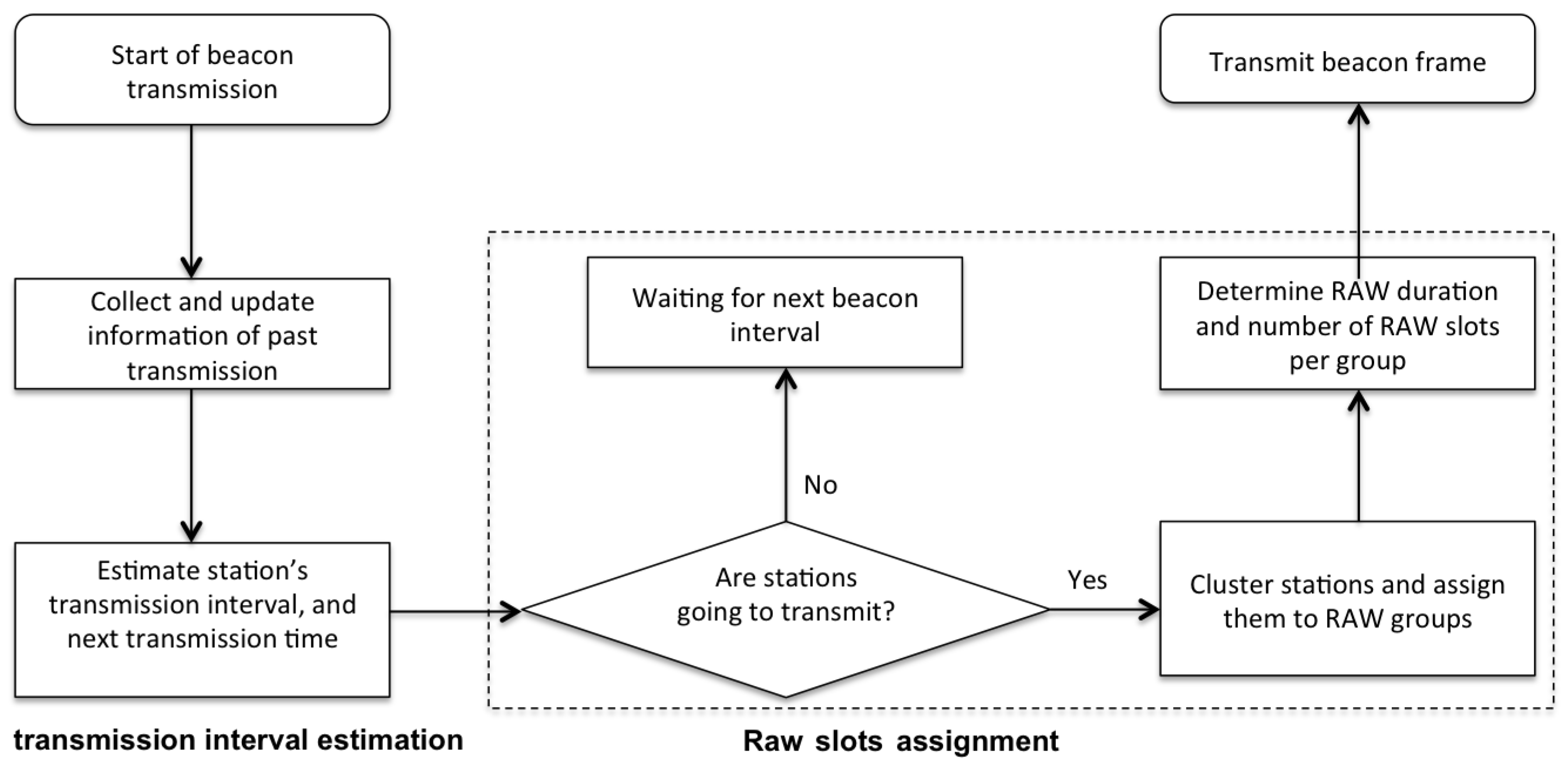
As depicted in
Figure 4, the algorithm is executed at each target beacon transmission time (TBTT), and consists of two main steps. First, the AP updates its estimation
of the packet transmission interval
of each station based on packet transmission information obtained during the last beacon interval. As the algorithm is optimized for sensor stations, it is assumed that each station transmits packets with a certain (predictable) frequency. However, as the estimation is updated at the start of each beacon interval, the algorithm can easily cope with changes in this transmission frequency over time. Second, TAROA determines the RAW parameters and assigns stations to RAW slots based on this estimated transmission frequency. Finally, the RAW parameters are transmitted to the stations by the AP in the RPS element of the beacon frame. The remainder of this section explains the two main steps of the algorithm (i.e., transmission interval estimation and RAW slot assignment).
4.3. Transmission Interval Estimation
The first main step of the algorithm is determining the estimated transmission interval and next transmission time for each station . As shown in Algorithm 1, they are estimated based on successful and failed transmissions during the previous beacon interval. A station’s transmission is regarded as successful if the AP received at least one packet from the station. If a station was assigned a RAW slot, but no packets were received by the AP during that slot, it is considered a failed transmission. The failed transmission can be be caused by the lack of packets in the station’s transmission queue, or by a collision or interference. The algorithm consists of three main blocks: (i) the previous transmission failed (lines 1–3); (ii) the previous transmission was successful, but the one before failed (lines 4–6); and (iii) the last two transmissions were successful (lines 7–16).
First, if the previous transmission failed, the transmission failure counter is increased by 1 (line 2). Additionally, this means that the estimated transmission interval of station s, is too short, as we assume s had no packets in its transmit queue. In reality, a transmission failure can also be caused by collisions. However, as RAW aims to minimize collisions, we can assume the probability of transmission failure caused by collision is low enough to be ignored. Increasing sharply could result in overestimation, which results in fewer packets being delivered to the AP and more packets being dropped due to the overflow of station’s transmission queue. Although increasing slowly can lead to a more accurate estimation, it may waste channel access time, as some stations will be assigned RAW slots without transmitting packets, while there will be no channel access time left for other stations that need it. For this reason, the increase of the estimated transmission interval follows the multiplicative-decrease principle of the Transmission Control Protocol (TCP) congestion control, and it is increased by the number of subsequent failed transmissions multiplied by two. As the number of failed transmission attempts increases, the algorithm assumes its estimation is more wrong and it will increase the interval faster.
In the second case (lines 4–6), the failure counter is set to 0 and the transmission interval is estimated as the time difference between the last two successful transmissions.
If an accurate is obtained in case 2, the next transmission will succeed and lead to case 3 (lines 7–16) in which the two last transmissions are successful. If only one packet is received (case 3.1), is updated in the same way as in case 2 (lines 9–10). If, on the other hand, is underestimated, s may transmit multiple packets to the AP (case 3.2, lines 11–12). In that case, the estimated transmission interval is reduced by 1 beacon interval (line 12). Finally, there are two more cases where the current estimated transmission interval is not larger than the beacon interval (i.e., ) and multiple packets were received from the station s by the AP (i.e., (cases 3.3 and 3.4). In case 3.3 (lines 13–14), the number of received packets is higher than the estimated number of expected packets (i.e., ) and the transmission interval is reduced by adding 1 to the inverse (line 14). Case 3.4 (lines 15–16) represents the inverse case, where fewer packets are received than estimated, and the transmission interval is increased by subtracting 1 from the inverse (line 16). Finally, the next transmission time is calculated as the last successful transmission plus the newly estimated transmission interval (line 17). In essence, the algorithm is iterative, and as more information about successful and failed transmissions becomes available, the estimate of will become more accurate.
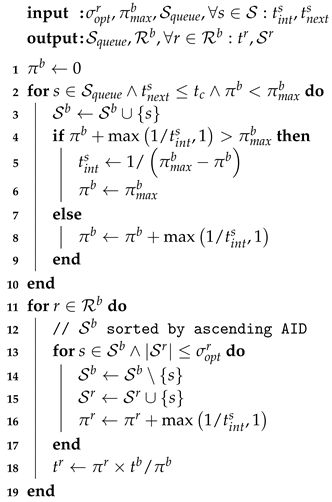
4.4. RAW Slot Assignment
The second main step of TAROA determines the set of RAW slots
to initialize in the next beacon interval
b, as well as for each of the RAW slots their duration
, and the assigned stations
. These RAW parameters are selected based on the previously determined estimation of the transmission interval
and next transmission time
. As shown in Algorithm 2, this is a two-step process: (i) select a subset of stations with pending packets to be assigned to a RAW slot during the upcoming beacon interval (lines 2–8); and (ii) partition the selected stations among the available number of RAW slots and determine the slot duration (lines 9–14).
| Algorithm 2: RAW parameter configuration for beacon interval b |
![Sensors 17 01559 i002]() |
In the first part (lines 2–8), the algorithm iterates over all stations s, according to ascending last successful transmission time (i.e., ) until the next station has a next estimated transmission time greater than the current time (i.e., ) or the maximum allowed number of packet transmissions has been reached (i.e., ) (line 2). The station is first added to the set of stations allowed to transmit during the beacon interval (line 3). Then, if the station is estimated to transmit more than one packet per beacon interval (i.e., ) and its estimated number of transmissions will exceed the maximum packet transmissions in b (line 4), then it is allowed to transmit part of its packets and its estimated transmission interval is updated accordingly (line 5). Otherwise, the station is expected to be able to transmit all of its packets and is increased with the number of packets s is estimated to transmit in the beacon interval (line 8).
At this point, it should be noted that all slots within a RAW group have the same duration and only stations with sequential AID can be assigned to the same group. Moreover, the optimal duration of a slot depends on the number of stations assigned to it, as well as their data rates, number of queued packets, and packet payload sizes. As such, for simplicity, we assume throughout the remainder of this paper that each RAW group has exactly one slot, allowing all slots to have a different size. Overcoming this problem is possible by selecting a worst-case slot duration (suboptimal) or performing dynamic AID reassignment. The latter is expected to increase optimality, but falls outside the scope of this paper.
In the second part (lines 9–14), stations are assigned to RAW slots
according to increasing AID (as only sequential AID can be assigned to the same group) until the number of stations assigned to the slot are greater or equal to the optimal number of assigned stations (i.e.,
) (line 10). How to calculate this optimum is explained in more detail in
Section 5. The number of packets to be transmitted by
s is added to the expected number of packet transmissions in
r (line 13). Finally, the optimal duration
of the slot is determined based on the number of expected packet transmission
(line 14).
7. Conclusions
In this paper, we propose a novel traffic-adaptive RAW optimization algorithm (TAROA) to adjust the RAW parameters in real time based on the current traffic conditions, optimized for sensor networks with mainly upstream traffic in which each station is assumed to transmit packets with a certain (predictable) frequency. The TAROA algorithm improves upon the state of art in three ways, including supporting dynamic and heterogeneous traffic conditions, only using information available on the AP side and real-time execution. The combination of these three factors allows TAROA to be deployed in realistic environment. The TAROA algorithm is executed at each target beacon transmission time (TBTT), it first estimates the packet transmission interval of each station only based on packet transmission information obtained during the last beacon interval, and then determines the RAW parameters and assigns stations to RAW slots based on this estimated transmission frequency.
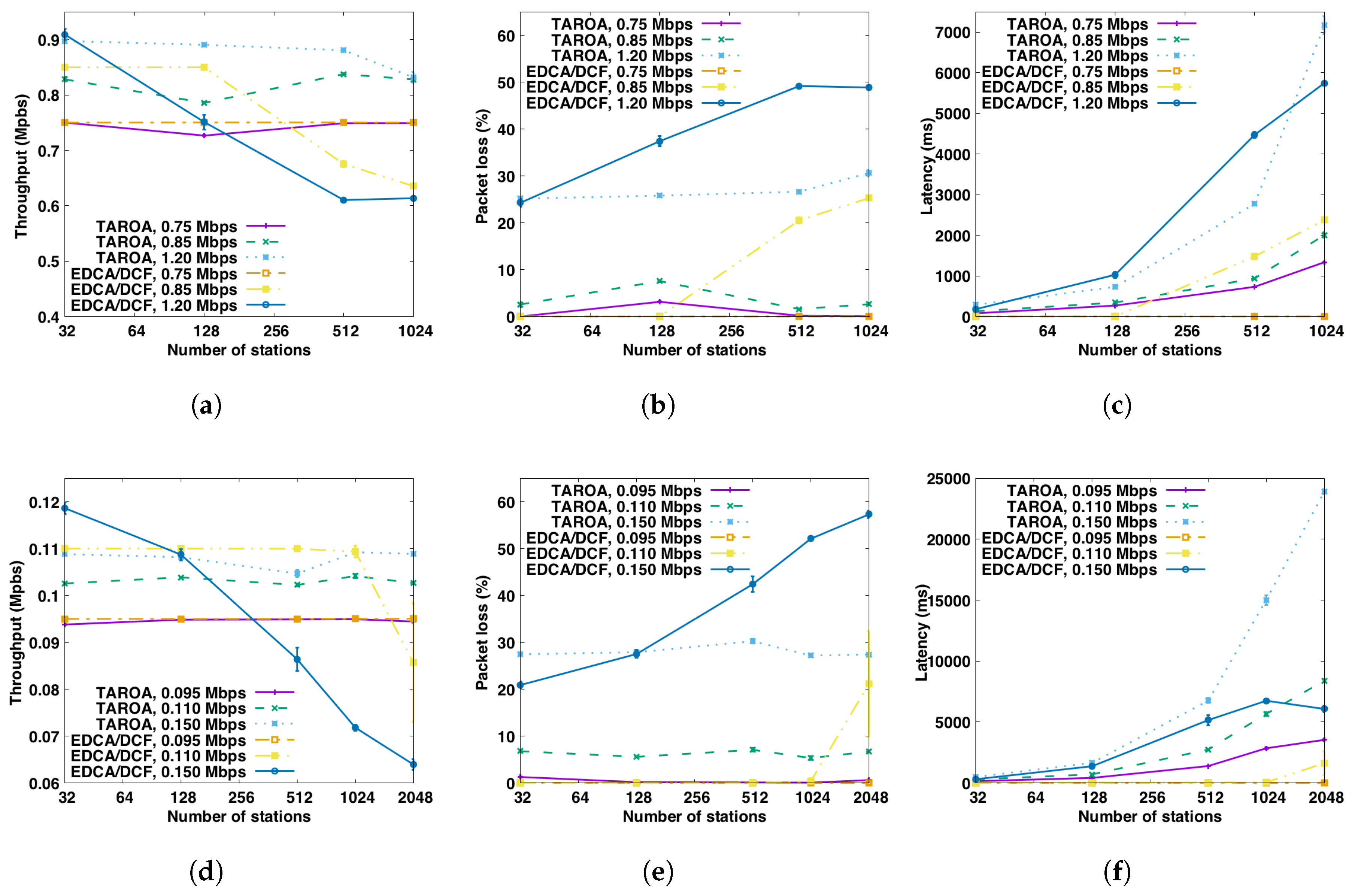
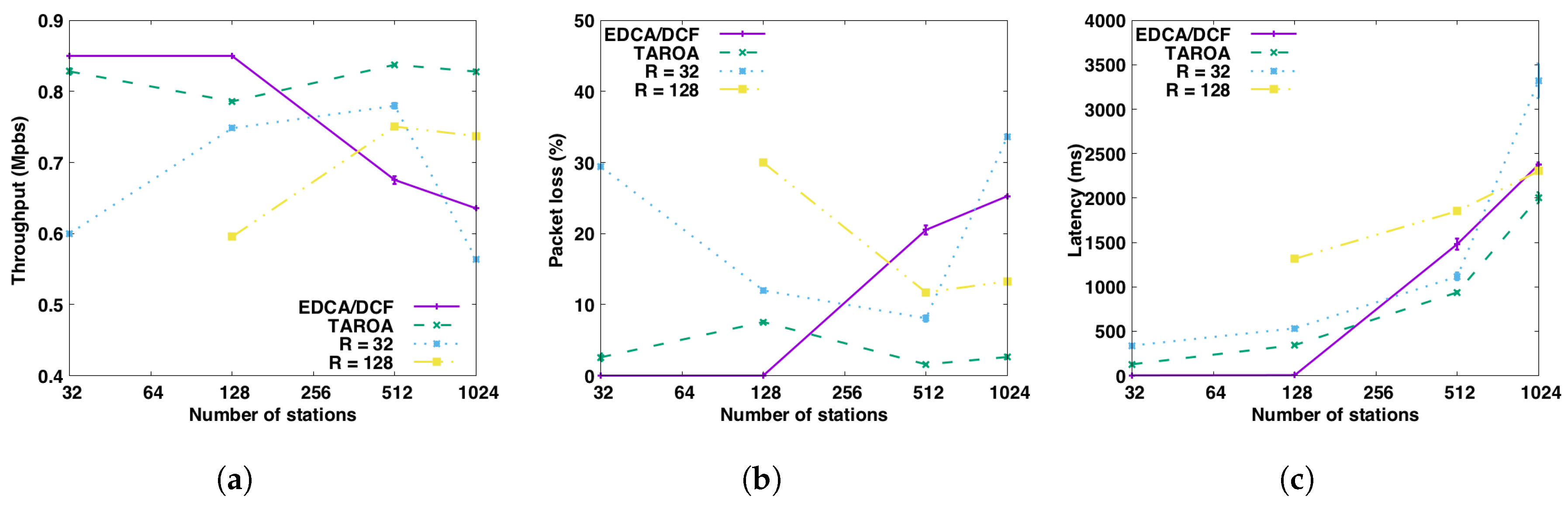
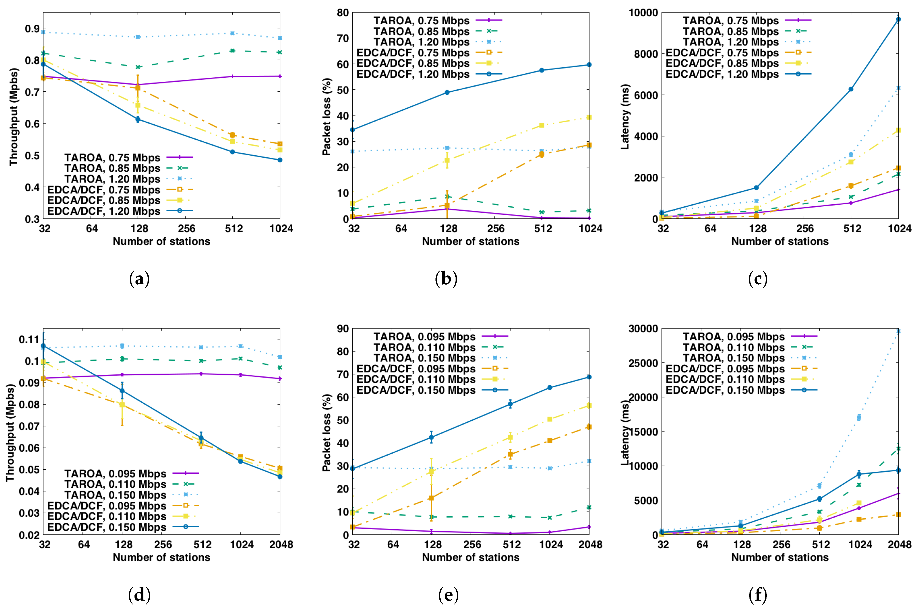
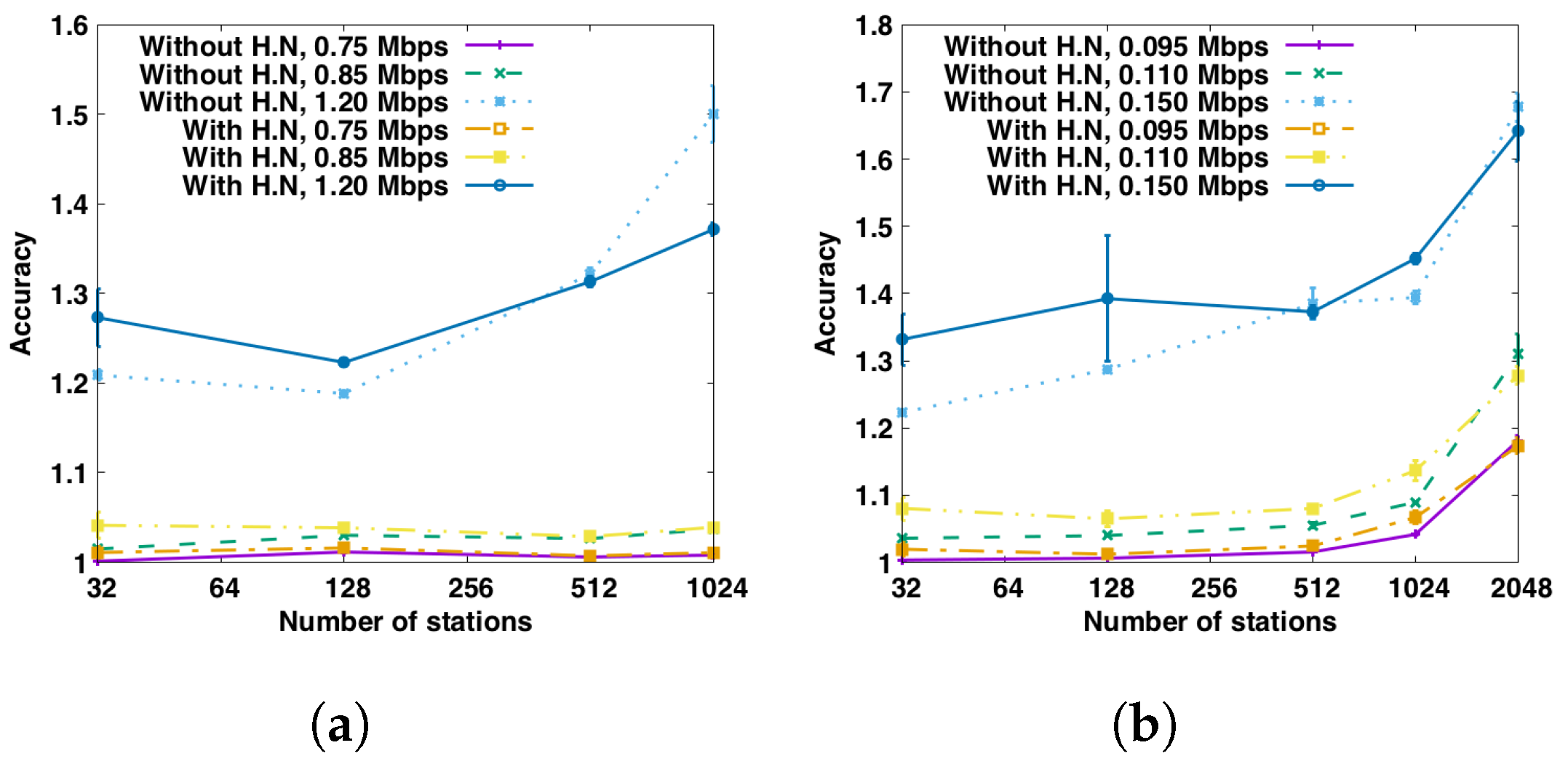
The simulation results reveal three key points on TAROA. First, it scales much better than EDCA/DCF in dense networks in terms of throughput under static traffic conditions. Second, it is resilient to dynamic traffic conditions in which topology or transmission interval change over time. In the scenario under evaluation, TAROA only starts to experience throughput degradation when topology changes at Poisson rate 5. Third, TAROA gains additional advantages over EDCA/DCF when hidden nodes are present under both static and dynamic traffic conditions. Hidden nodes highly degrade the performance of EDCA/DCF, while TAROA is hardly affected. In summary, for dense IoT networks, TAROA can easily adapt to current traffic conditions in real time and significantly improves throughput.
In future work, we will further improve the performance of the TAROA algorithm, and, in particular, the traffic estimation under high load. Moreover, TAROA will be extended to support adaptive MCS.


