
Time-Frequency Analysis of Non-Stationary Biological Signals with Sparse Linear Regression Based Fourier Linear Combiner


Abstract
:1. Introduction
2. Methodology
2.1. Model of Sparse-BMFLC
2.2. ADMM Solution for Sparse-BMFLC
2.3. Time-Frequency Decomposition from Sparse-BMFLC
3. Results
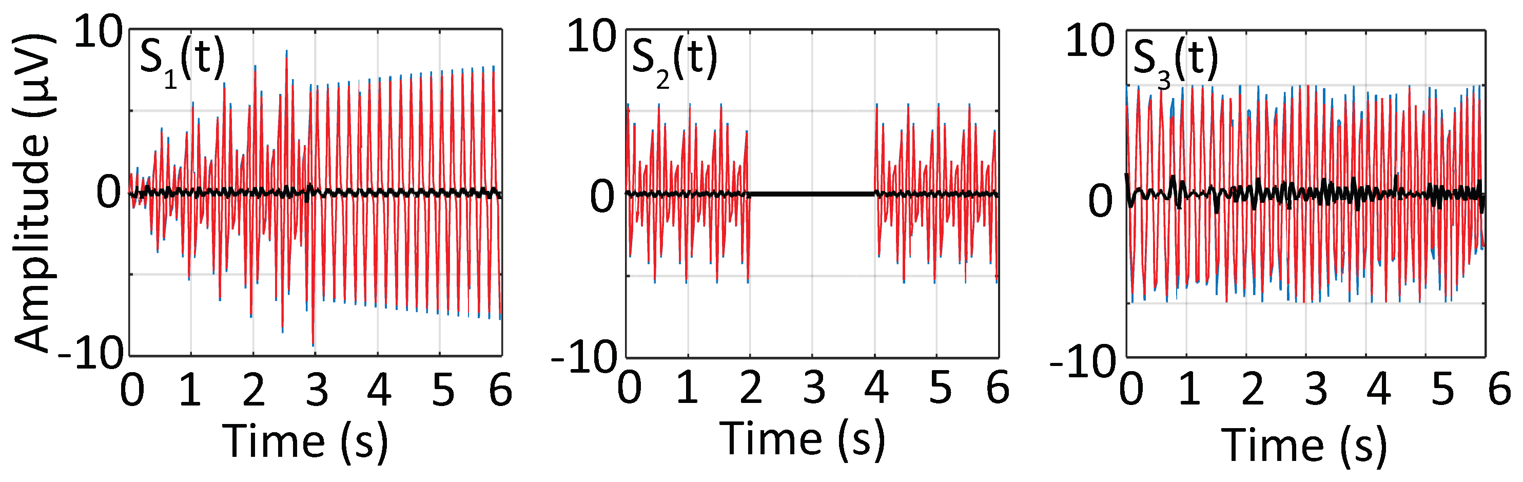
3.1. Synthetic Signal
3.2. Parameter Selection
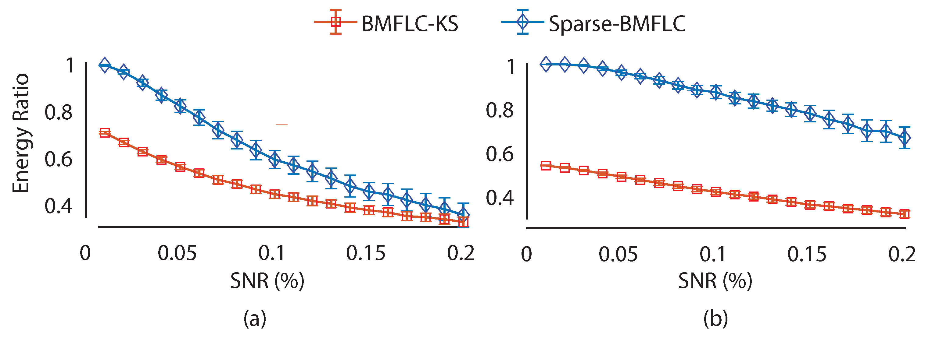
3.3. Estimation Performance of Sparse-BMFLC
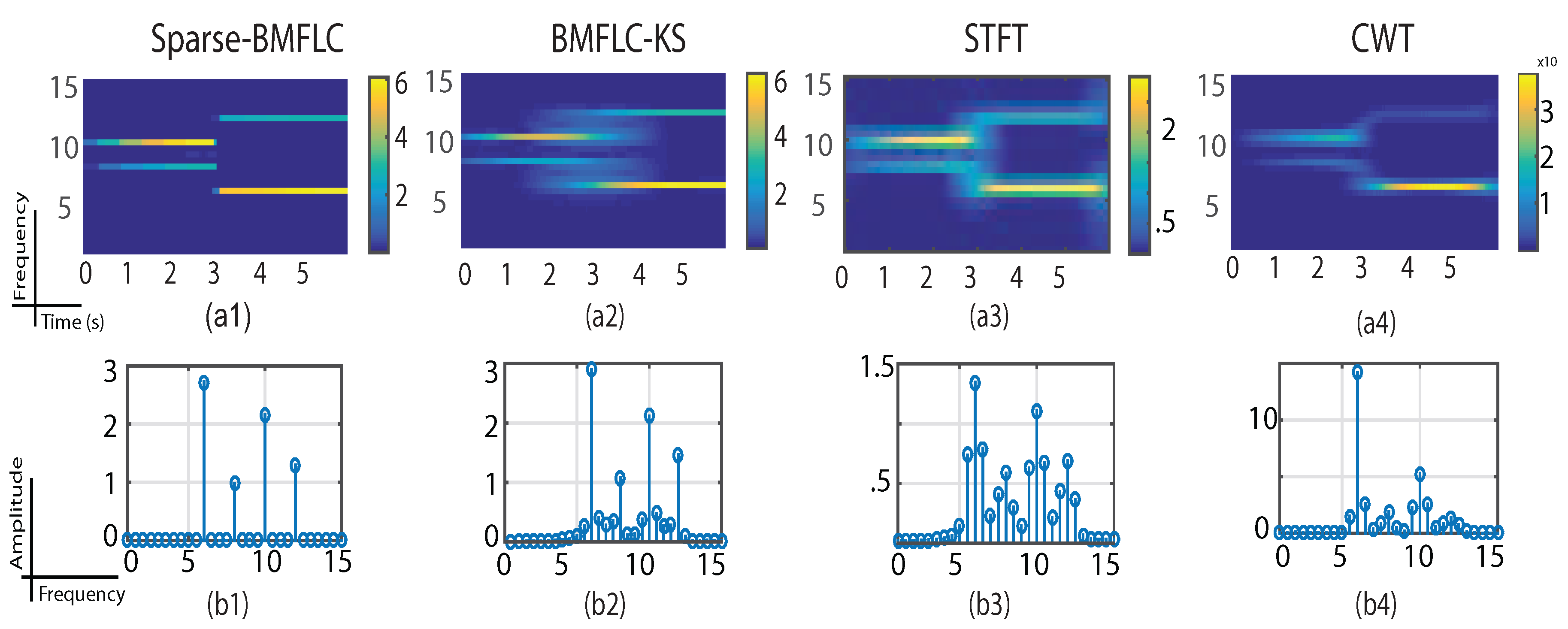
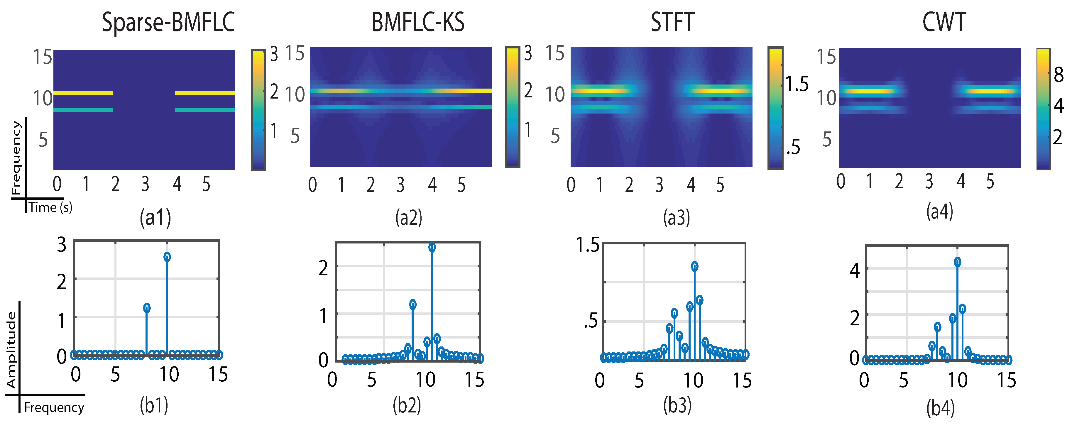
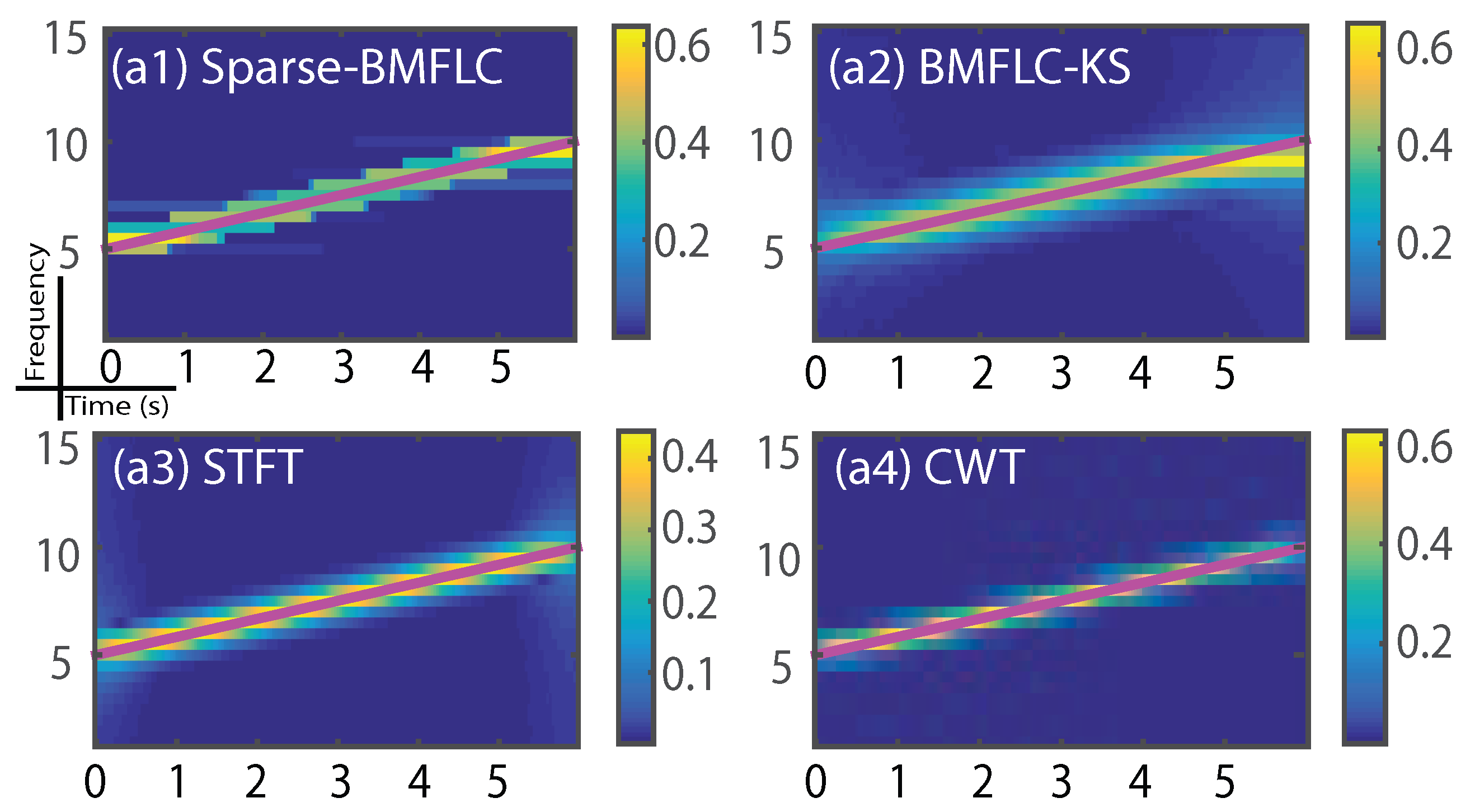
3.4. Time-Frequency Decomposition of the Synthesized Signal
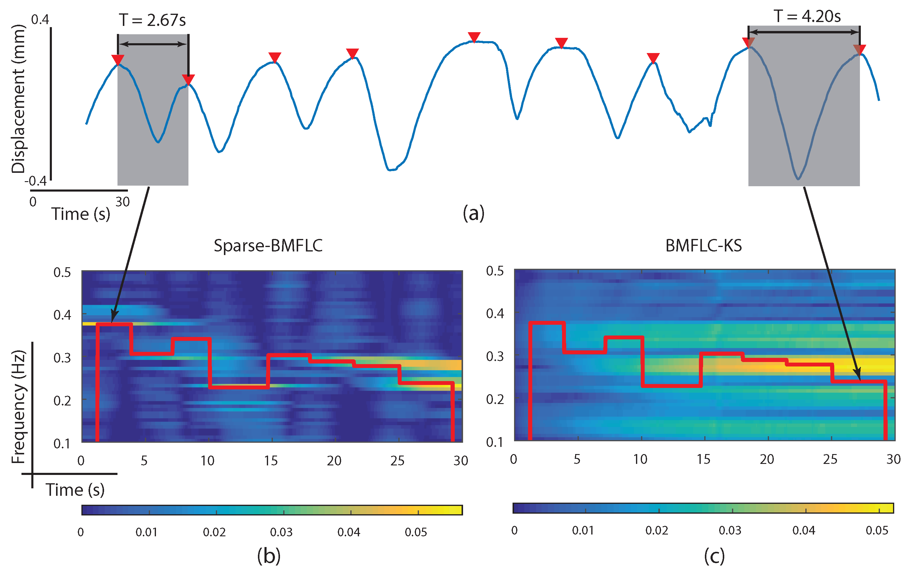
3.5. Time-Frequency Decomposition of Respiratory Motion Signal
4. Discussion
5. Conclusions
Acknowledgments
Author Contributions
Conflicts of Interest
References
- Gallego, J.A.; Rocon, E.; Roa, J.O.; Moreno, J.C.; Pons, J.L. Real-time estimation of pathological tremor parameters from gyroscope data. Sensors 2010, 10, 2129–2149. [Google Scholar] [CrossRef] [PubMed]
- Shafiq, G.; Tatinati, S.; Ang, W.T.; Veluvolu, K.C. Automatic Identification of Systolic Time Intervals in Seismocardiogram. Sci. Rep. 2016, 6, 37524. [Google Scholar] [CrossRef] [PubMed]
- Shafiq, G.; Veluvolu, K.C. Surface chest motion decomposition for cardiovascular monitoring. Sci. Rep. 2014, 4, 5093. [Google Scholar] [CrossRef] [PubMed]
- Veluvolu, K.C.; Ang, W.T. Estimation of physiological tremor from accelerometers for real-time applications. Sensors 2011, 11, 3020–3036. [Google Scholar] [CrossRef] [PubMed]
- Tarvainen, M.P.; Georgiadis, S.; Lipponen, J.A.; Hakkarainen, M.; Karjalainen, P.A. Time-varying spectrum estimation of heart rate variability signals with Kalman smoother algorithm. Conf. Proc. IEEE Eng. Med. Biol. Soc. 2009, 2009, 1–4. [Google Scholar] [PubMed]
- Allen, D.P.; MacKinnon, C.D. Time Frequency analysis of movement-related spectral power in EEG during repetitive movements: A comparison of methods. J. Neurosci. Methods 2010, 186, 107–115. [Google Scholar] [CrossRef] [PubMed]
- Gonuguntla, V.; Wang, Y.; Veluvolu, K.C. Event-related functional network identification: Application to EEG classification. IEEE J. Sel. Topics Signal Process. 2016, 10, 1284–1294. [Google Scholar] [CrossRef]
- Aboy, M.; Marquez, O.W.; McNames, J.; Hornero, R.; Trong, T.; Goldstein, B. Adaptive Modeling and Spectral Estimation of Nonstationary Biomedical Signals Based on Kalman Filtering. IEEE Trans. Biomed. Eng. 2005, 52, 1485–1489. [Google Scholar] [CrossRef] [PubMed]
- Zhang, Z.; Chan, S.C.; Wang, C. A New regularized adaptive windowed lomb periodogram for time-frequency analysis of nonstationary signals with impulsive components. IEEE Trans. Instrum. Meas. 2012, 61, 2283–2304. [Google Scholar] [CrossRef]
- Laguna, P.; Moody, G.B.; Mark, R.G. Power spectral density of unevenly sampled data by least-square analysis: Performance and application to heart rate signals. IEEE Trans. Biomed. Eng. 1998, 45, 698–715. [Google Scholar] [CrossRef] [PubMed]
- Mallat, S. A Wavelet Tour of Signal Processing; Elsevier: Amsterdam, The Netherlands, 2009. [Google Scholar]
- Aguiar-Conraia, L.; Soares, M.J. The Continuous Wavelet Transform: A Primer. NIPE WP 2011, 16, 1–46. [Google Scholar]
- Torrence, C.; Compo, G.P. A Practical Guide to Wavelet Analysis. Bull. Am. Meteorol. Soc. 1998, 79, 61–78. [Google Scholar] [CrossRef]
- Shumway, R.H.; Stoffer, D.S. Time Series Analysis and Its Applications; Springer Texts in Statistics; Springer: New York, NY, USA, 2011. [Google Scholar]
- Tarvainen, M.P.; Hiltunen, J.K.; Ranta-aho, P.O.; Karjalainen, P.A. Estimation of nonstationary EEG with Kalman smoother approach: An application to event-related synchronization (ERS). IEEE Trans. Biomed. Eng. 2004, 51, 516–524. [Google Scholar] [CrossRef] [PubMed]
- Simon, D. Optimal State Estimation; Wiley: Hoboken, NJ, USA, 2006. [Google Scholar]
- Khan, M.E.; Dutt, D.N. An Expectation-Maximization Algorithm Based Kalman Smoother Approach for Event-Related Desynchronization (ERD) Estimation from EEG. IEEE Trans. Biomed. Eng. 2007, 54, 1191–1198. [Google Scholar] [CrossRef] [PubMed]
- Ting, C.M.; Salleh, S.H.; Zainuddin, Z.Z.; Bahar, A. Spectral Estimation of Nonstationary EEG Using Particle Filtering With Application to Event-Related Desynchronization (ERD). IEEE Trans. Biomed. Eng. 2011, 58, 321–331. [Google Scholar] [CrossRef] [PubMed]
- Wang, Y.; Veluvolu, K.C.; Cho, J.; Defoort, M. Adaptive Estimation of EEG for Subject-Specific Reactive Band Identification and Improved ERD Detection. Neurosci. Lett. 2012, 528, 137–142. [Google Scholar] [CrossRef] [PubMed]
- Veluvolu, K.C.; Wang, Y.; Kavuri, S.S. Adaptive Estimation of EEG-Rhythms for Optimal Band Identification in BCI. J. Neurosci. Methods 2012, 203, 163–172. [Google Scholar] [CrossRef] [PubMed]
- Wang, Y.; Veluvolu, K.C.; Lee, M. Time-Frequency Analysis of Band-Limited EEG with BMFLC and Kalman Filter for BCI Applications. J. NeuroEng. Rehabil. 2013, 10, 109. [Google Scholar] [CrossRef] [PubMed]
- Chen, S.S.; Donoho, D.L. Application of basis pursuit in spectrum estimation. In Proceedings of the 1998 IEEE International Conference on Acoustics, Speech and Signal Processing, Seattle, WA, USA, 15 May 1998; pp. 1865–1868. [Google Scholar]
- Li, E.; Shafiee, M.J.; Kazemzadeh, F.; Wong, A. Sparse reconstruction of compressed sensing multispectral data using a cross-spectral multilayered conditional random field model. In Proceedings of the SPIE 9599, Applications of Digital Image Processing XXXVIII, San Diego, CA, USA, 4 September 2015. [Google Scholar]
- Wunder, G.; Boche, H.; Strohmer, T.; Jung, P. Sparse Signal Processing Concepts for Efficient 5G System Design. IEEE Signal Proc. Mag. 2009, 3, 1–17. [Google Scholar] [CrossRef]
- Zahedi, R.; Krakow, L.W.; Chong, E.K.P.; Pezeshki, A. Adaptive estimation of time-varying sparse signals. IEEE Access 2013, 1, 449–464. [Google Scholar] [CrossRef]
- Angelosante, D.; Giannakis, G.B.; Sidiropoulos, N.D. Sparse Parametric Models for Robust Nonstationary Signal Analysis. IEEE Signal Proc. Mag. 2013, 30, 64–73. [Google Scholar] [CrossRef]
- Angelosante, D.; Giannakis, G.B.; Sidiropoulos, N.D. Estimating Multiple Frequency-Hopping Signal Parameters via Sparse Linear Regression. IEEE Trans. Signal Proc. 2010, 58, 5044–5056. [Google Scholar] [CrossRef]
- Li, Y.; Wei, H.L.; Billings, S.A. Identification of Time-Varying Systems Using Multi-Wavelet Basis Functions. IEEE Trans. Control Syst. Technol. 2011, 19, 656–663. [Google Scholar] [CrossRef]
- Billings, S.A.; Wei, H.L. Sparse Model Identification Using a Forward Orthogonal Regression Algorithm Aided by Mutual Information. IEEE Trans. Neural Netw. 2007, 18, 306–310. [Google Scholar] [CrossRef] [PubMed]
- Shechtman, Y.; Beck, A.; Eldar, Y.C. GESPAR: Efficient Phase Retrieval of Sparse Signals. IEEE Trans. Signal Proc. 2014, 62, 928–938. [Google Scholar] [CrossRef]
- Hastie, T.; Tibshirani, R.; Friedman, J. The Elements of Statistical Learning; Springer: Berlin, Germany, 2008. [Google Scholar]
- Tibshirani, R.; Saunders, M.; Rosset, S.; Zhu, J.; Knight, K. Sparsity and smoothness via the fused lasso. J. R. Stat. Soc Ser. B 2005, 67, 91–108. [Google Scholar] [CrossRef]
- Boyd, S.; Parikh, N.; Chu, E.; Peleato, B.; Eckstein, J. Distributed Optimization and Statistical Learning via the Alternating Direction Method of Multipliers. Found. Trends Mach. Learn. 2010, 3, 1–122. [Google Scholar] [CrossRef]
- Bertsekas, D.P.; Tsitsiklis, J.N. Parallel and Distributed Computation: Numerical Methods; Athena Scientiic: Belmont, MA, USA, 1997. [Google Scholar]
- Zhu, X.; Chen, W.; Nemoto, T.; Kanemitsu, Y.; Kitamura, K.I.; Yamakoshi, K.I.; Wei, D. Real-time monitoring of respiration rhythm and pulse rate during sleep. IEEE Trans. Biomed. Eng. 2006, 53, 2553–2563. [Google Scholar] [PubMed]
- Wasserman, K.; Whipp, B.J.; Koyal, S.N.; Beaver, W.L. Anaerobic Threshold and Repiratory Gas Exchange during Exercise. J. Appl. Physiol. 1973, 35, 239–243. [Google Scholar]
- Holley, K.; MacNabb, C.M.; Georgiadis, P.; Minasyan, H.; Shukla, A.; Mathews, D. Monitoring minute ventilation versus respiratory rate to measure the adequacy of ventilation in patients undergoing upper endoscopic procedures. J. Clin. Monit. Comput. 2016, 30, 33–39. [Google Scholar] [CrossRef] [PubMed]
- Brown, T.E.; Beightol, L.A.; Koh, J.; Eckberg, D.L. Important influence of respiration on human R-R interval power spectra is largely ignored. J. Appl. Physiol. 1993, 75, 2310–2317. [Google Scholar] [PubMed]
- Chon, K.H.; Dash, S.; Ju, K. Estimation of Respiratory Rate From Photoplethysmogram Data Using Time-Frequency Spectral Estimation. IEEE Trans. Biomed. Eng. 2009, 56, 2054–2063. [Google Scholar] [CrossRef] [PubMed]
- Ernst, F.; Dürichen, R.; Schlaefer, A.; Schweikard, A. Evaluating and comparing algorithms for respiratory motion prediction. Phys. Med. Biol. 2013, 58, 3911–3929. [Google Scholar] [CrossRef] [PubMed]


| Methods | |||
|---|---|---|---|
| BMFLC-KS | 2.12% | 3.01% | 3.00% |
| Sparse-BMFLC | 5.12% | 3.95% | 9.59% |
| Synthetic Signal | BMFLC-KS | Sparse-BMFLC | CWT | STFT |
|---|---|---|---|---|
| 0.7328 | 0.9972 | 0.5961 | 0.4151 | |
| 0.5596 | 0.9981 | 0.4819 | 0.3492 |
© 2017 by the authors. Licensee MDPI, Basel, Switzerland. This article is an open access article distributed under the terms and conditions of the Creative Commons Attribution (CC BY) license (http://creativecommons.org/licenses/by/4.0/).
Share and Cite
Wang, Y.; Veluvolu, K.C. Time-Frequency Analysis of Non-Stationary Biological Signals with Sparse Linear Regression Based Fourier Linear Combiner. Sensors 2017, 17, 1386. https://doi.org/10.3390/s17061386
Wang Y, Veluvolu KC. Time-Frequency Analysis of Non-Stationary Biological Signals with Sparse Linear Regression Based Fourier Linear Combiner. Sensors. 2017; 17(6):1386. https://doi.org/10.3390/s17061386
Chicago/Turabian StyleWang, Yubo, and Kalyana C. Veluvolu. 2017. "Time-Frequency Analysis of Non-Stationary Biological Signals with Sparse Linear Regression Based Fourier Linear Combiner" Sensors 17, no. 6: 1386. https://doi.org/10.3390/s17061386
APA StyleWang, Y., & Veluvolu, K. C. (2017). Time-Frequency Analysis of Non-Stationary Biological Signals with Sparse Linear Regression Based Fourier Linear Combiner. Sensors, 17(6), 1386. https://doi.org/10.3390/s17061386