
Sensor Fusion Based on an Integrated Neural Network and Probability Density Function (PDF) Dual Kalman Filter for On-Line Estimation of Vehicle Parameters and States

 ,
,  , ,
, ,
Abstract
:1. Introduction
- estimates, simultaneously and on-line, the vehicle’s states and parameters.
- uses a simplified vehicle model,
- is useful in all kinds of environments (tunnels, urban and forested driving environments),
- uses signals of sensors installed on-board in current vehicles,
- takes into consideration both the measurements and model errors.
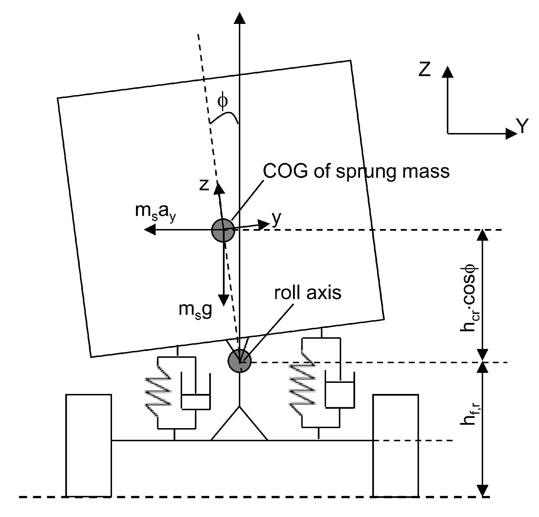
2. Vehicle Model
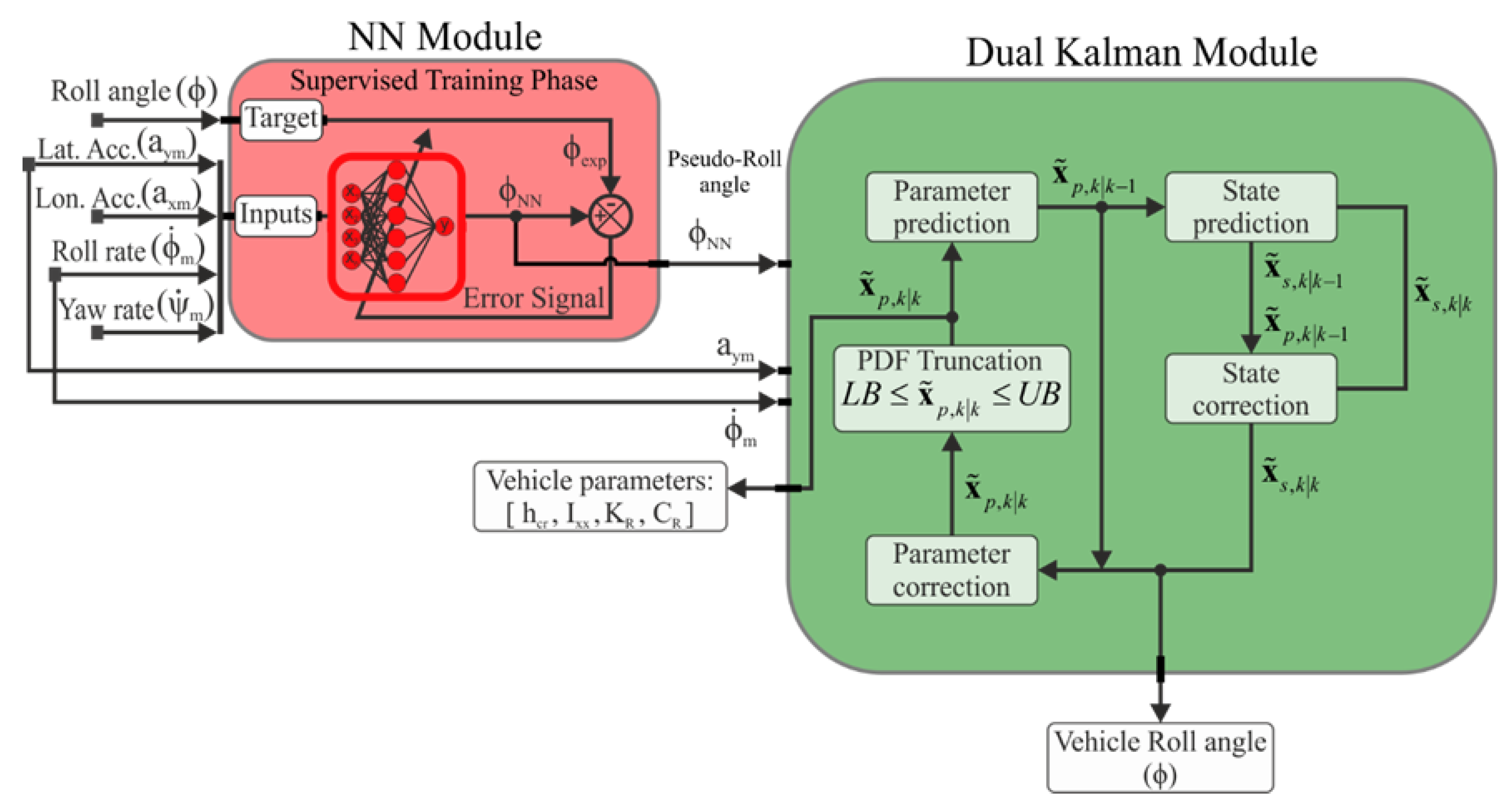
3. Vehicle’s Parameters and Roll Angle Estimation
3.1. DKF Module
- Parameter prediction:
- State prediction:
- State correction:
- Parameter correction:
3.2. PDF Truncation Approach
- For i = 1 to i = p, the mean and variance of the parameter state are calculated by means of the following equations:and are calculated from the Jordan canonical decomposition of (see Appendix A), that fulfills the condition stated by the equation:is an orthogonal matrix obtained by using Gram–Schmidt orthogonalization that satisfies (see Appendix B):The vector has mean 0 and an identity covariance matrix. Hence, its elements are statistically independent of one another. Only the first element of is constrained, therefore, the PDF truncation is reduced to a one-dimensional truncation:where is the truncated mean value given by the following expression:and is the truncated covariance given by the following equation:whereThe truncated PDF is normalized to achieve a unity area, and the fist element of is constrained:so that,
- Finally, the final constrained parameter estimate and covariance at time k is given by:
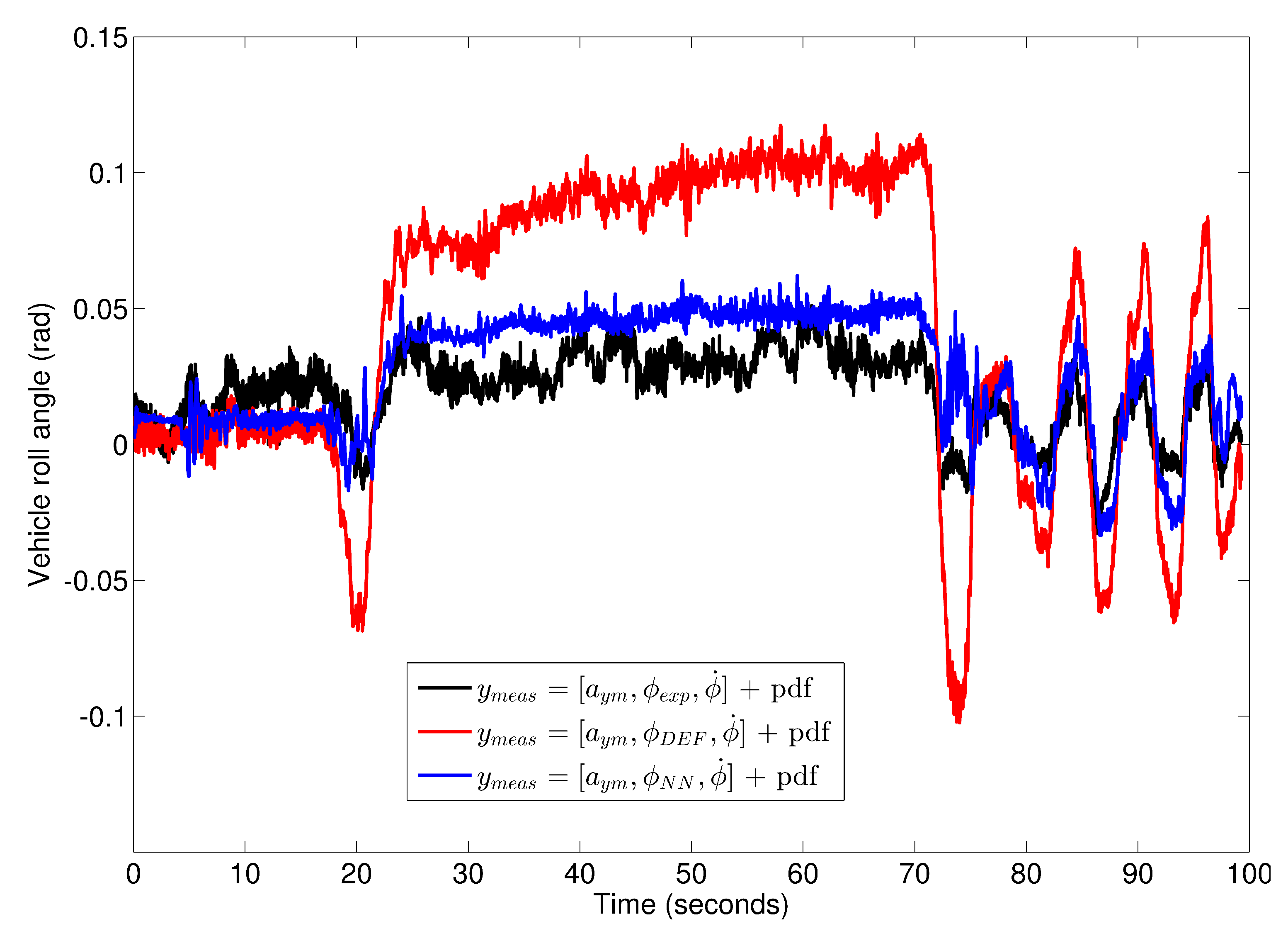
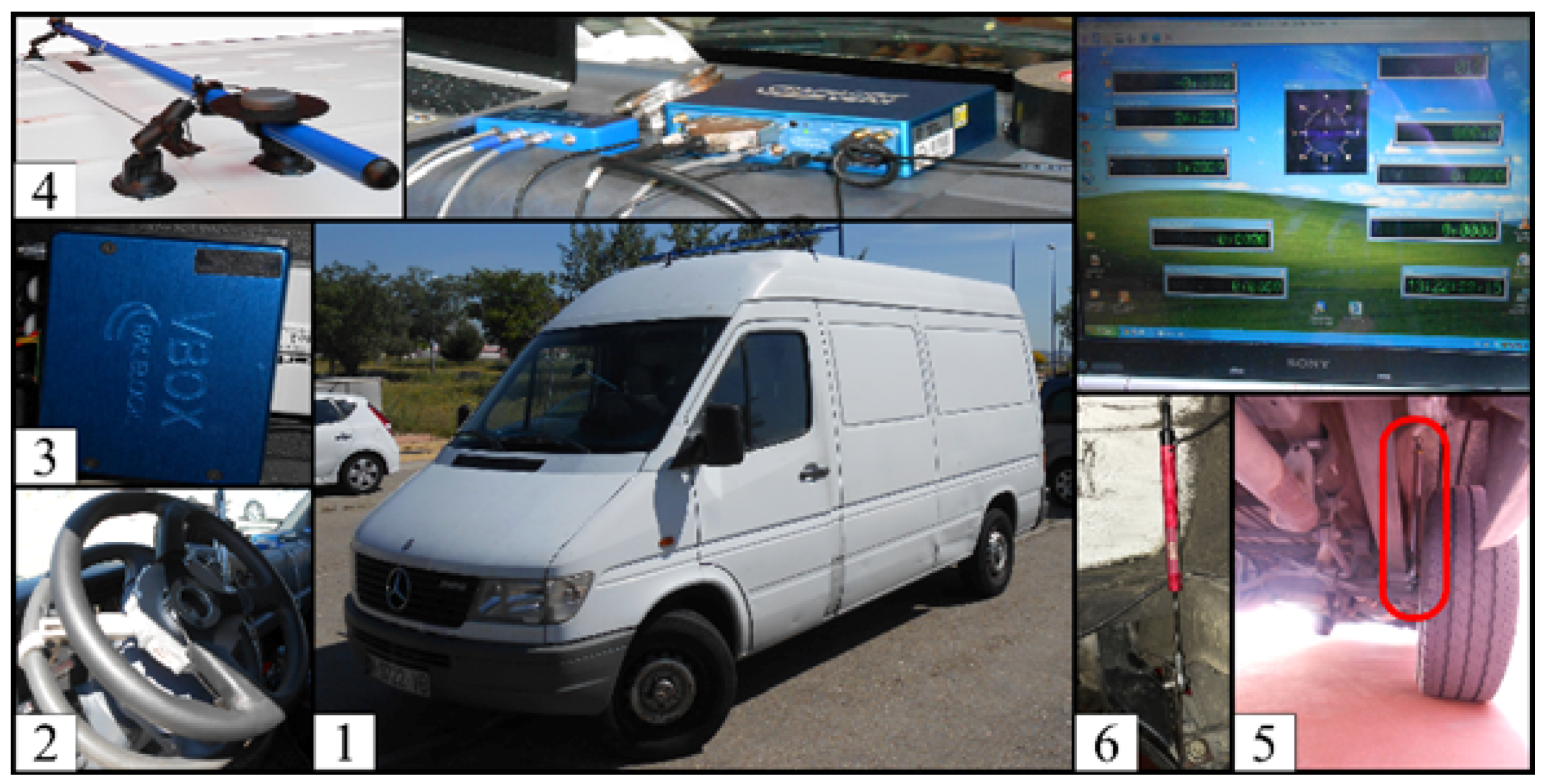
4. Experimental Results and Discussion
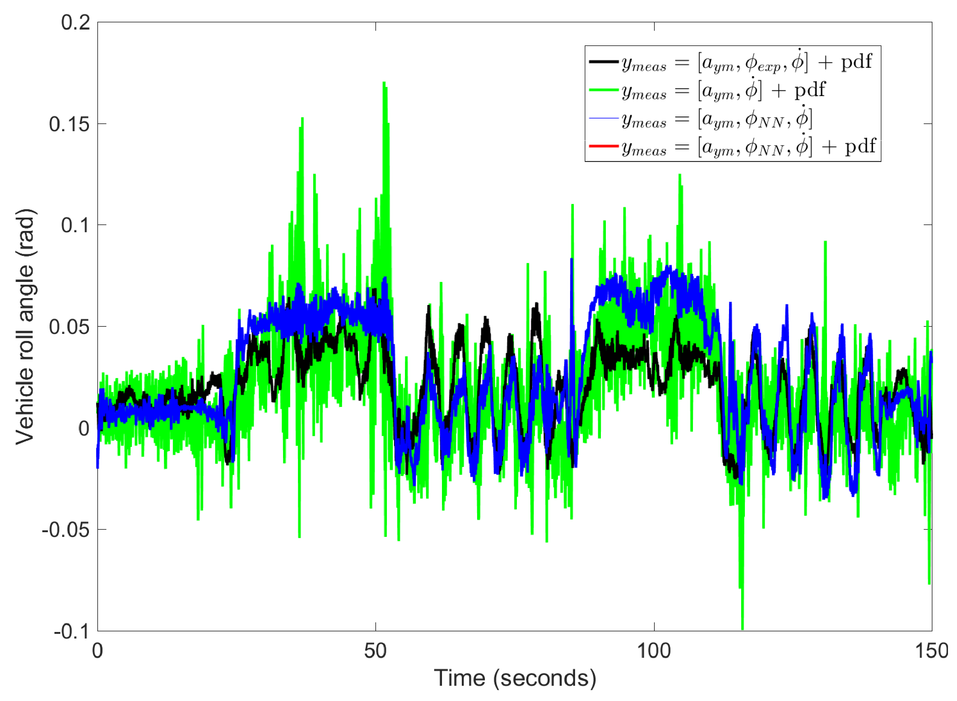
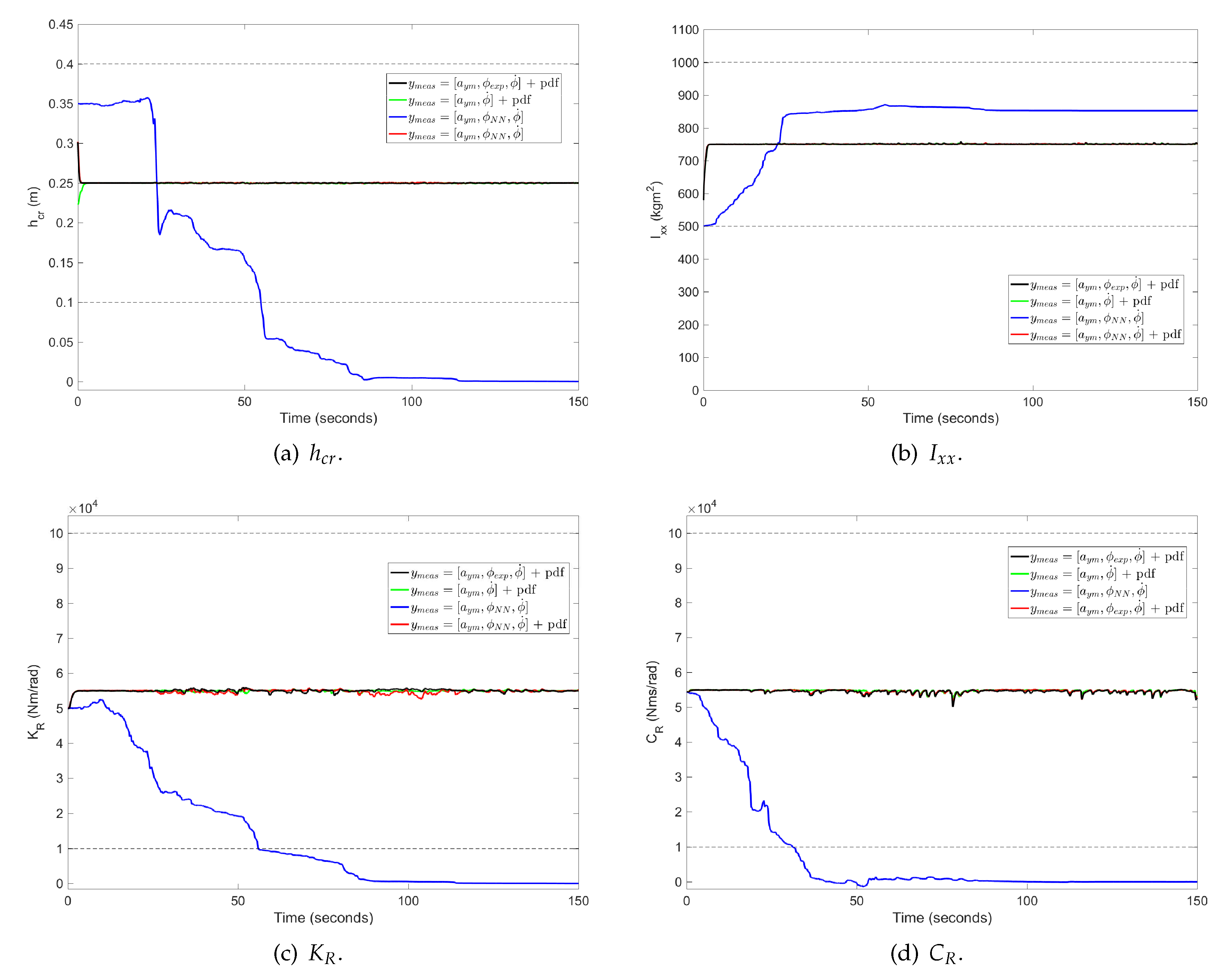
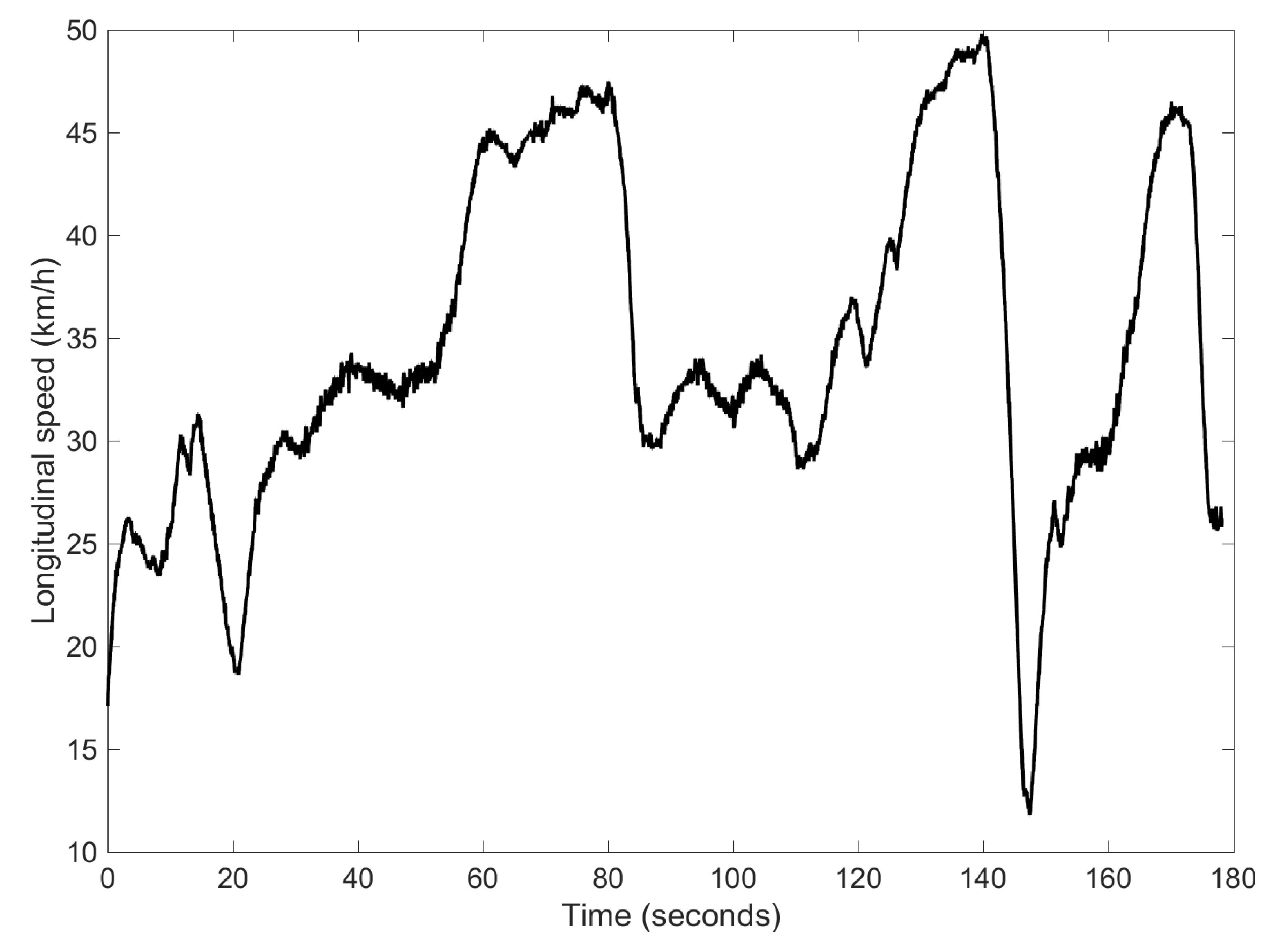
4.1. Case 1: Combination of Slalom and J-Turn Maneouvres
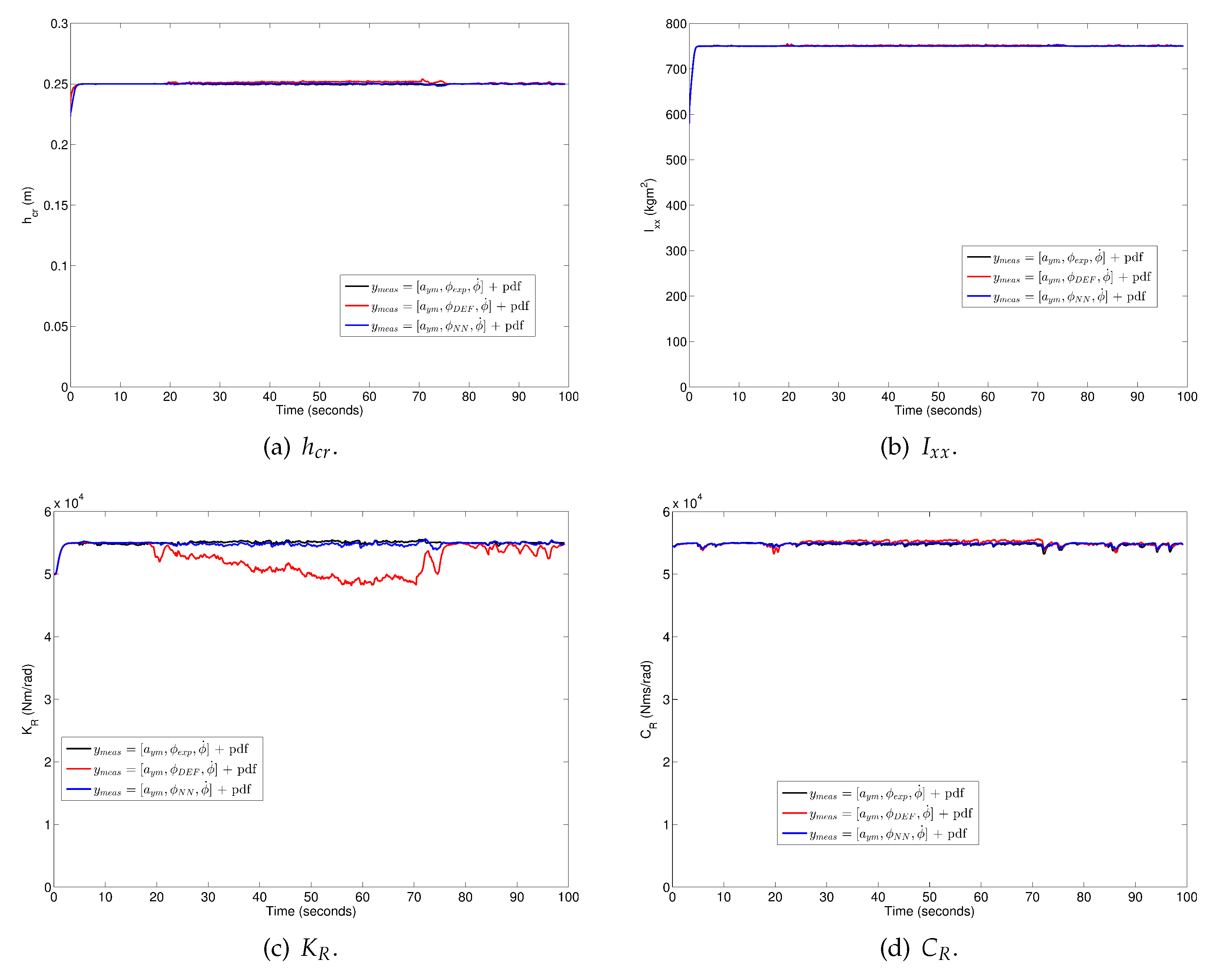
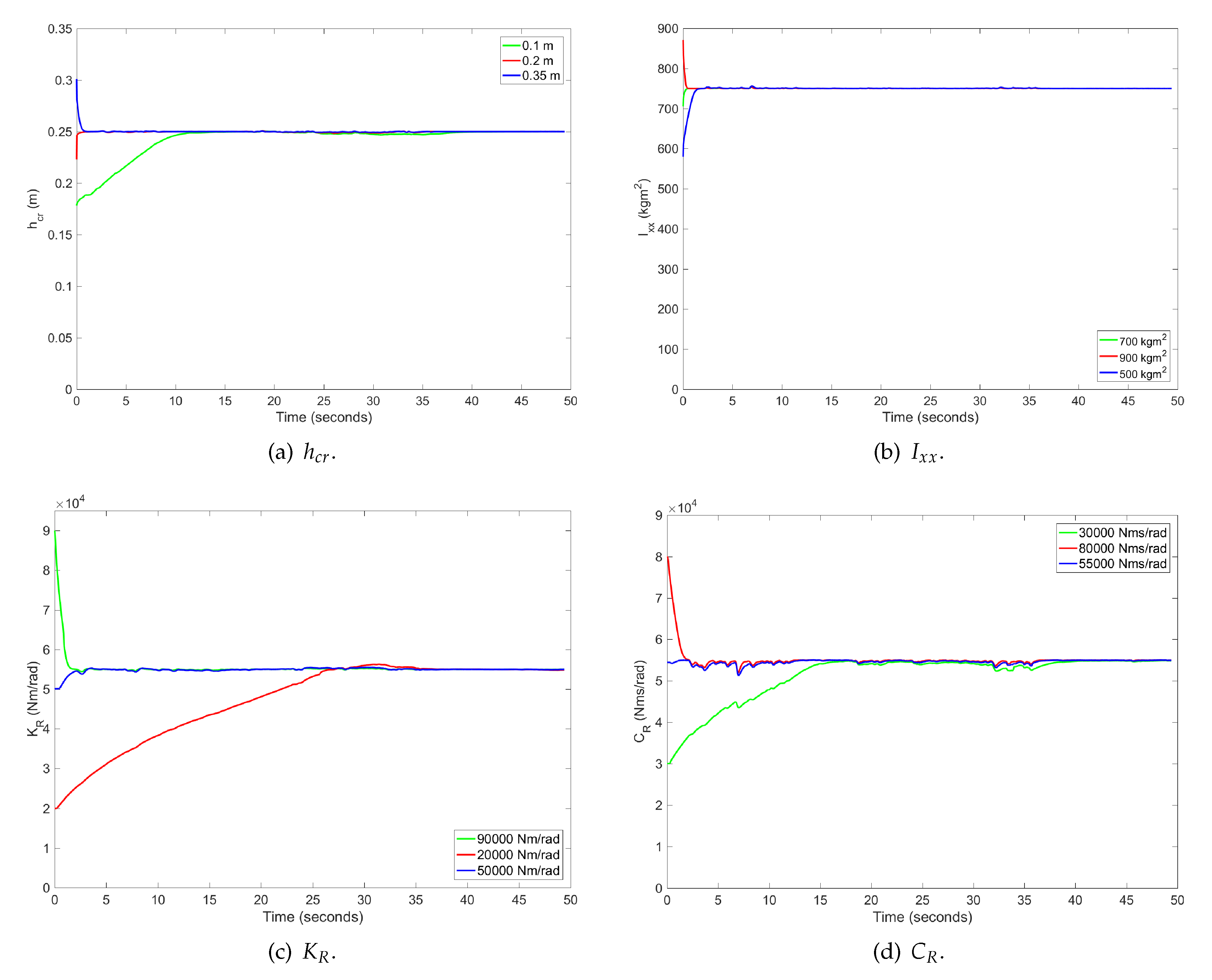
4.2. Case 2: DLC and J-Turn Manoeuvres
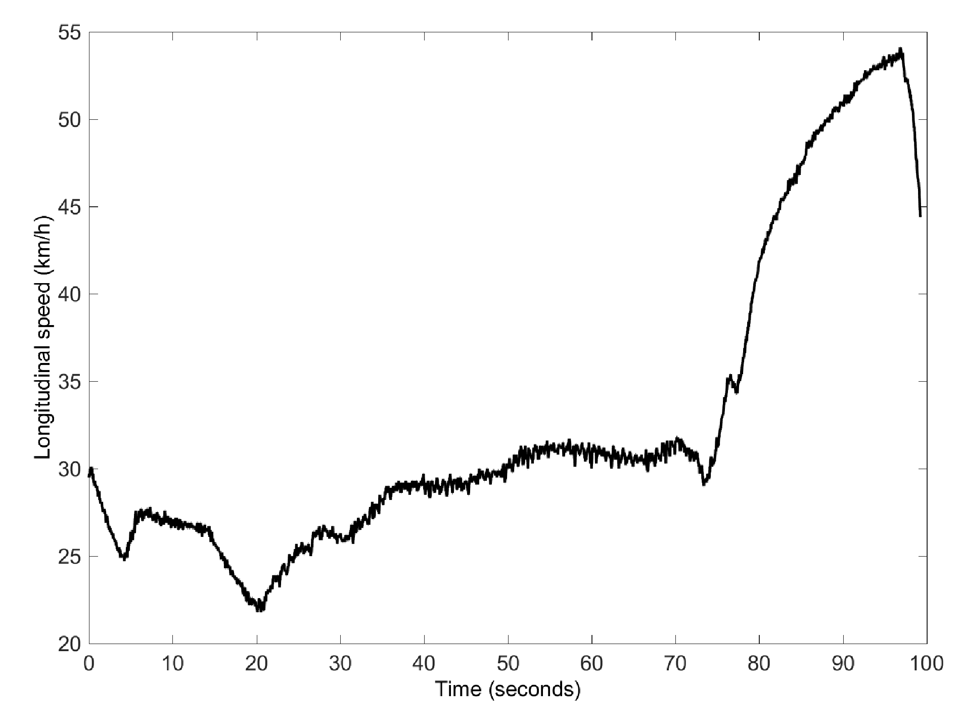
4.3. Case 3: Slalom and J-Turn Manoeuvres
5. Conclusions
Acknowledgments
Author Contributions
Conflicts of Interest
Abbreviations
| COG | Center of fravity |
| DLC | Double lane change |
| DKF | Dual Kalman filter |
| GPS | Global positioning system |
| IMU | Inertial measurement unit |
| NN | Neural networks |
| Probability density function |
Appendix A. Jordan Canonical Decomposition
Appendix B. Gram–Schmidt Orthogonalization Algorithm
- For , suppose that is a matrix, where n is the number of estimate parameter, with rows :The first row of is computed as:
- For :
- (a)
- Compute :where is a vector that is an n-element column vector comprised entirely of zeros, except that its kth element is a 1.
- (b)
- if , then replace it with:
- (c)
- Normalize :
References
- Hickman, J.S.; Guo, F.; Camden, M.C.; Hanowski, R.J.; Medina, A.; Erin Mabry, J. Efficacy of roll stability control and lane departure warning systems using carrier-collected data. J. Saf. Res. 2015, 52, 59–63. [Google Scholar] [CrossRef] [PubMed]
- Boada, M.J.L.; Boada, B.L.; Gauchia, A.; Calvo, J.A.; Diaz, V. Active roll control using reinforcement learning for a single unit heavy vehicle. Int. J. Heavy Veh. Syst. 2009, 16, 412–430. [Google Scholar] [CrossRef]
- Rajamani, R.; Piyabongkarn, D.; Tsourapas, V.; Lew, J.Y. Real-time estimation of roll angle and CG height for active rollover prevention applications. In Proceedings of the 2009 American Control Conference, St. Louis, MO, USA, 10–12 June 2009; pp. 433–438. [Google Scholar]
- Tafner, R.; Reichhartinger, M.; Horn, M. Robust online roll dynamics identification of a vehicle using sliding mode concepts. Control Eng. Pract. 2014, 29, 235–246. [Google Scholar] [CrossRef]
- Eric, T.H.; Li, X.; Hrovat, D. Estimation of land vehicle roll and pitch angles. Veh. Syst. Dyn. 2007, 45, 433–443. [Google Scholar] [CrossRef]
- Doumiati, M.; Baffet, G.; Lechner, D.; Victorino, A.; Charara, A. Embedded estimation of the tire/road forces and validation in a laboratory vehicle. In Proceedings of the 9th International Symposium on Advanced Vehicle Control, Kobe, Japan, 6–9 October 2008; pp. 533–538. [Google Scholar]
- Vargas-Meléndez, L.; Boada, B.; Boada, M.J.L.; Gauchía, A.; Díaz, V. A Sensor Fusion Method Based on an Integrated Neural Network and Kalman Filter for Vehicle Roll Angle Estimation. Sensors 2016, 16, 1400. [Google Scholar] [CrossRef] [PubMed]
- Bevly, D.M.; Ryu, J.; Gerdes, J.C. Integrating INS Sensors with GPS Measurements for Continuous Estimation of Vehicle Sideslip, Roll, and Tire Cornering Stiffness. IEEE Trans. Intell. Transp. Syst. 2006, 7, 483–493. [Google Scholar] [CrossRef]
- Jo, K.; Chu, K.; Sunwoo, M. Interacting Multiple Model Filter-Based Sensor Fusion of GPS with In-Vehicle Sensors for Real-Time Vehicle Positioning. IEEE Trans. Intell. Transp. Syst. 2012, 13, 329–343. [Google Scholar] [CrossRef]
- Nam, K.; Oh, S.; Fujimoto, H.; Hori, Y. Estimation of Sideslip and Roll Angles of Electric Vehicles Using Lateral Tire Force Sensors Through RLS and Kalman Filter Approaches. IEEE Trans. Ind. Electron. 2013, 60, 988–1000. [Google Scholar] [CrossRef]
- Zhang, S.; Yu, S.; Liu, C.; Yuan, X.; Liu, S. A Dual-Linear Kalman Filter for Real-Time Orientation Determination System Using Low-Cost MEMS Sensors. Sensors 2016, 16, 264. [Google Scholar] [CrossRef] [PubMed]
- Burkul, S.R.; Pawar, P.R.; Jagtap, K.R. Estimation of vehicle parameters using Kalman Filter: Review. Int. J. Curr. Eng. Technol. 2014, 4, 2731–2735. [Google Scholar]
- Hong, S.; Lee, C.; Borrelli, F.; Hedrick, J.K. A Novel Approach for Vehicle Inertial Parameter Identification Using a Dual Kalman Filter. IEEE Trans. Intell. Transp. Syst. 2015, 16, 151–161. [Google Scholar] [CrossRef]
- Nada, E.; Ahmed, A.; Abd-Alla, M.A. Modified Dual Unscented Kalman Filter Approach For Measuring Vehicle States And Vehicle Parameters. Int. J. Eng. Res. Technol. 2014, 3, 1423–1430. [Google Scholar]
- Reina, G.; Paianom, M.; Blanco-Claraco, J.L. Vehicle parameter estimation using a model-based estimator. Mech. Syst. Signal Process. 2017, 87, 227–241. [Google Scholar] [CrossRef]
- Simon, D. Optimal State Estimation: Kalman, H Infinity, and Nonlinear Approaches; John Wiley Publishing House: Hoboken, NJ, USA, 2007. [Google Scholar]
- Yang, C.; Blasch, E. Kalman Filtering with Nonlinear State Constraints. In Proceedings of the 2006 9th International Conference on Information Fusion, Florence, Italy, 10–13 July 2006; pp. 1–8. [Google Scholar]
- Simon, D.; Chia, T. Kalman Filtering with State Equality Constraints. IEEE Trans. Aerosp. Electron. Syst. 2002, 39, 128–136. [Google Scholar] [CrossRef]
- Shimada, N.; Shirai, Y.; Kuno, Y.; Miura, J. Hand gesture estimation and model refinement using monocular camera-ambiguity limitation by inequality constraints. In Proceedings of the Third IEEE International Conference on Automatic Face and Gesture Recognition, Nara, Japan, 14–16 April 1998; pp. 268–273. [Google Scholar]
- Simon, D.; Simon, D.L. Aircraft Turbofan Engine Health Estimation Using Constrained Kalman Filtering. J. Eng. Gas Turbines Power 2005, 127, 323–328. [Google Scholar] [CrossRef]
- Tully, S.; Kantor, G.; Choset, H. Inequality constrained Kalman filtering for the localization and registration of a surgical robot. In Proceedings of the 2011 IEEE/RSJ International Conference on Intelligent Robots and Systems (IROS), San Francisco, CA, USA, 25–30 September 2011. [Google Scholar]
- Boada, B.L.; Garcia-Pozuelo, D.; Boada, M.J.L.; Diaz, V. A Constrained Dual Kalman Filter Based on PDF Truncation for Estimation of Vehicle Parameters and Road Bank Angle: Analysis and Experimental Validation. IEEE Trans. Intell. Transp. Syst. 2017, 18, 1006–1016. [Google Scholar] [CrossRef]
- Kamnik, R.; Boettiger, F.; Hunt, K. Roll dynamics and lateral load transfer estimation in articulated heavy freight vehicles. Proc. Inst. Mech. Eng. Part D J. Automob. Eng. 2003, 217, 985–997. [Google Scholar] [CrossRef]
- Doumiati, M.; Victorino, A.; Lechner, D.; Baffet, G.; Charara, A. Observers for vehicle tyre/road forces estimation: Experimental validation. Veh. Syst. Dyn. 2010, 48, 1345–1378. [Google Scholar] [CrossRef]
- Eric, A.; Wan, E.A.; Nelson, A.T. Dual Kalman Filtering Methods for Nonlinear Prediction, Smoothing, and Estimation. In Advances in Neural Information Processing Systems 9; MIT Press: Cambridge, MA, USA, 1997. [Google Scholar]
- Wenzel, T.A.; Burnham, K.J.; Blundell, M.V.; Williams, R.A. Dual extended Kalman filter for vehicle state and parameter estimation. Veh. Syst. Dyn. 2006, 44, 153–171. [Google Scholar] [CrossRef]
- Boada, M.J.L.; Calvo, J.A.; Boada, B.L.; Díaz, V. Modeling of a magnetorheological damper by recursive lazy learning. Int. J. Non-Linear Mech. 2011, 46, 479–485. [Google Scholar] [CrossRef]


| Parameter | Initial Values | ||
|---|---|---|---|
| Case 2.a | Case 2.b | Case 2.c | |
| (m) | 0.1 | 0.2 | 0.35 |
| (kg m) | 700 | 900 | 500 |
| (Nm/rad) | 90,000 | 20,000 | 50,000 |
| (Nms/rad) | 30,000 | 80,000 | 55,000 |
© 2017 by the authors. Licensee MDPI, Basel, Switzerland. This article is an open access article distributed under the terms and conditions of the Creative Commons Attribution (CC BY) license (http://creativecommons.org/licenses/by/4.0/).
Share and Cite
Vargas-Melendez, L.; Boada, B.L.; Boada, M.J.L.; Gauchia, A.; Diaz, V. Sensor Fusion Based on an Integrated Neural Network and Probability Density Function (PDF) Dual Kalman Filter for On-Line Estimation of Vehicle Parameters and States. Sensors 2017, 17, 987. https://doi.org/10.3390/s17050987
Vargas-Melendez L, Boada BL, Boada MJL, Gauchia A, Diaz V. Sensor Fusion Based on an Integrated Neural Network and Probability Density Function (PDF) Dual Kalman Filter for On-Line Estimation of Vehicle Parameters and States. Sensors. 2017; 17(5):987. https://doi.org/10.3390/s17050987
Chicago/Turabian StyleVargas-Melendez, Leandro, Beatriz L. Boada, Maria Jesus L. Boada, Antonio Gauchia, and Vicente Diaz. 2017. "Sensor Fusion Based on an Integrated Neural Network and Probability Density Function (PDF) Dual Kalman Filter for On-Line Estimation of Vehicle Parameters and States" Sensors 17, no. 5: 987. https://doi.org/10.3390/s17050987
APA StyleVargas-Melendez, L., Boada, B. L., Boada, M. J. L., Gauchia, A., & Diaz, V. (2017). Sensor Fusion Based on an Integrated Neural Network and Probability Density Function (PDF) Dual Kalman Filter for On-Line Estimation of Vehicle Parameters and States. Sensors, 17(5), 987. https://doi.org/10.3390/s17050987