
Comprehensive and Highly Accurate Measurements of Crane Runways, Profiles and Fastenings

Abstract
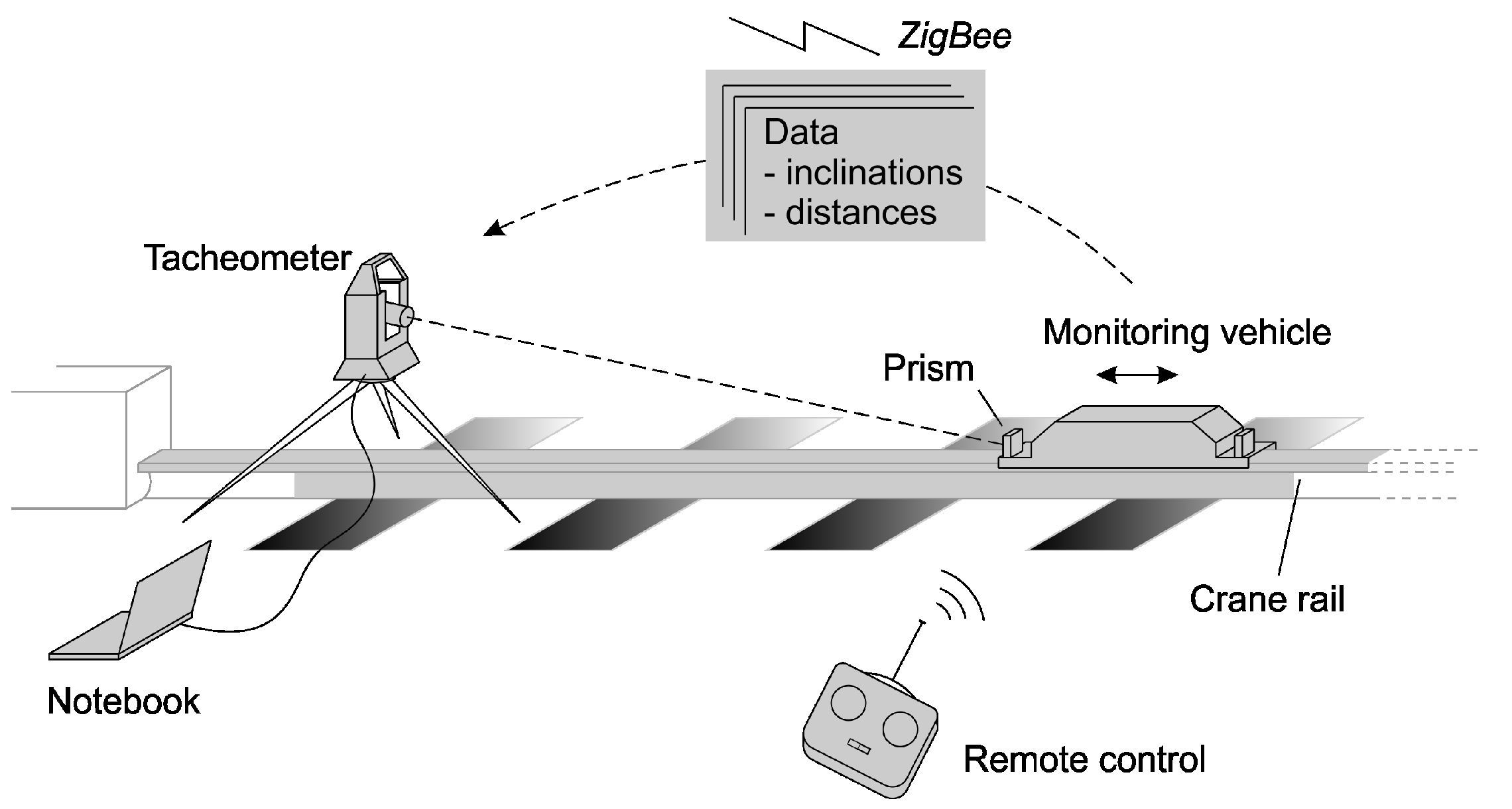
:1. Introduction
2. Definition of New Target Values for Crane Runways
2.1. Theoretical and Practical Rail Axis
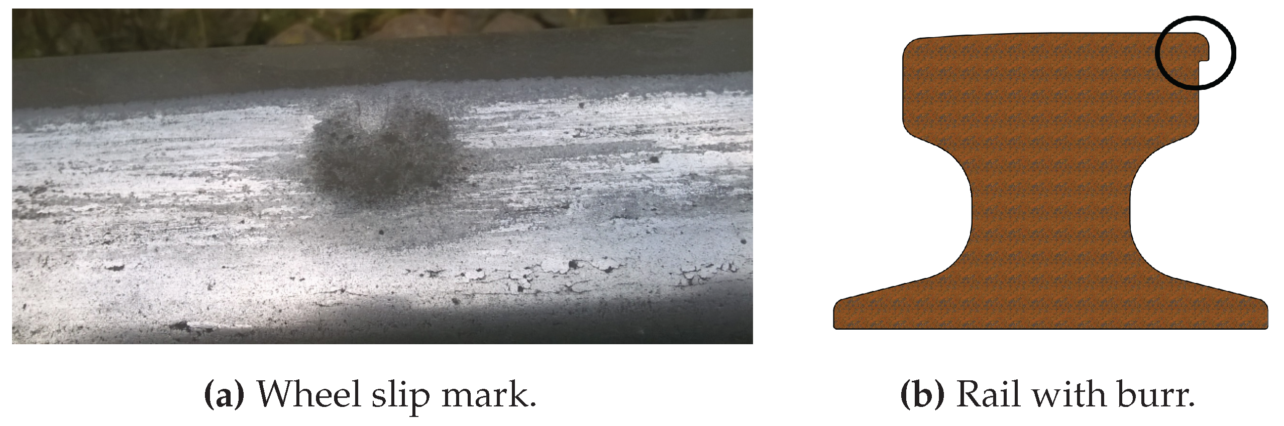
2.2. Defects of the Rail Profile
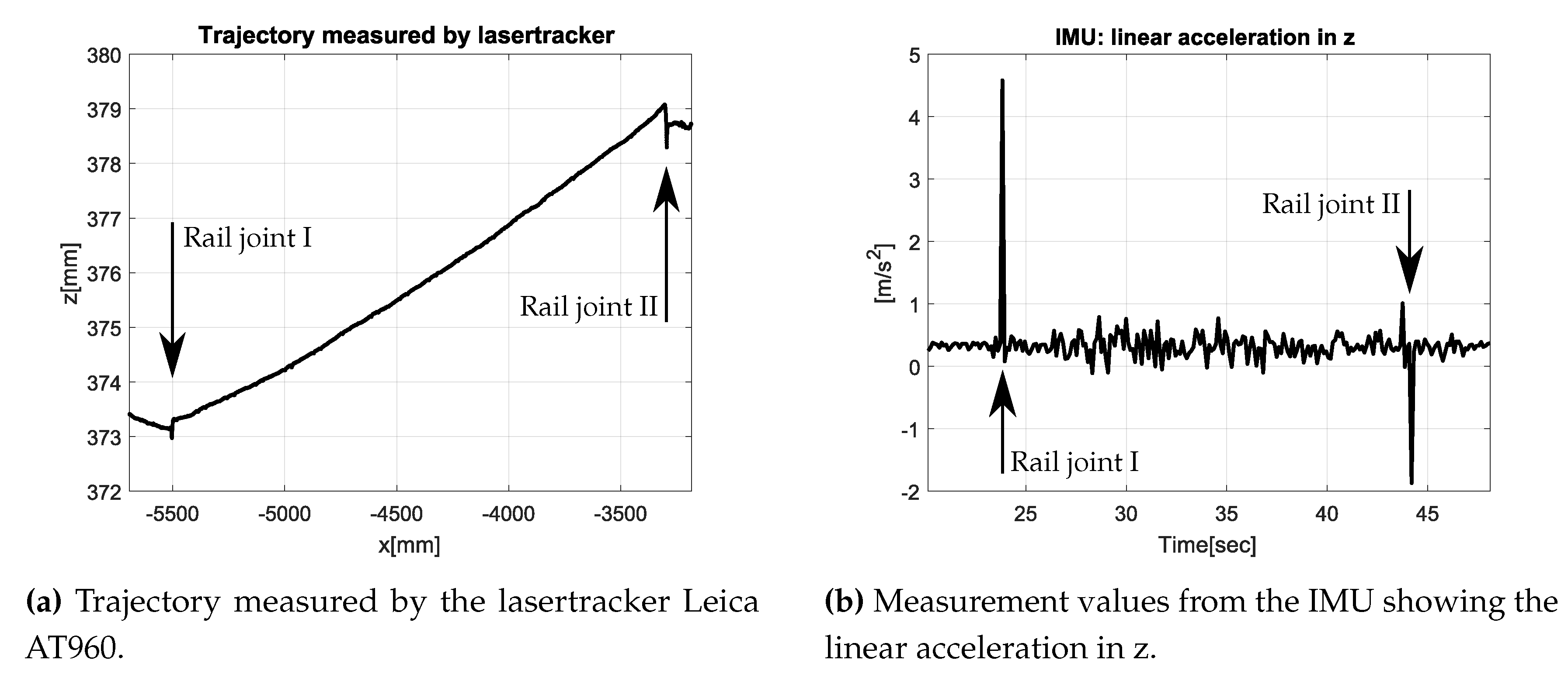
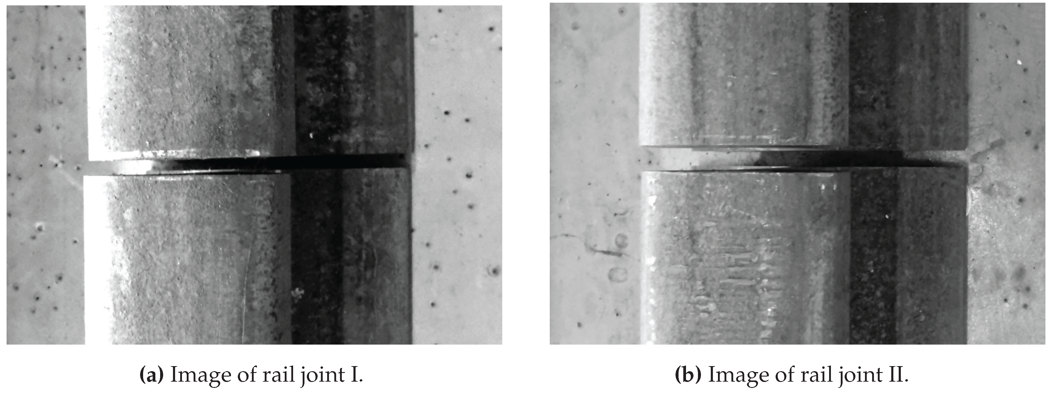
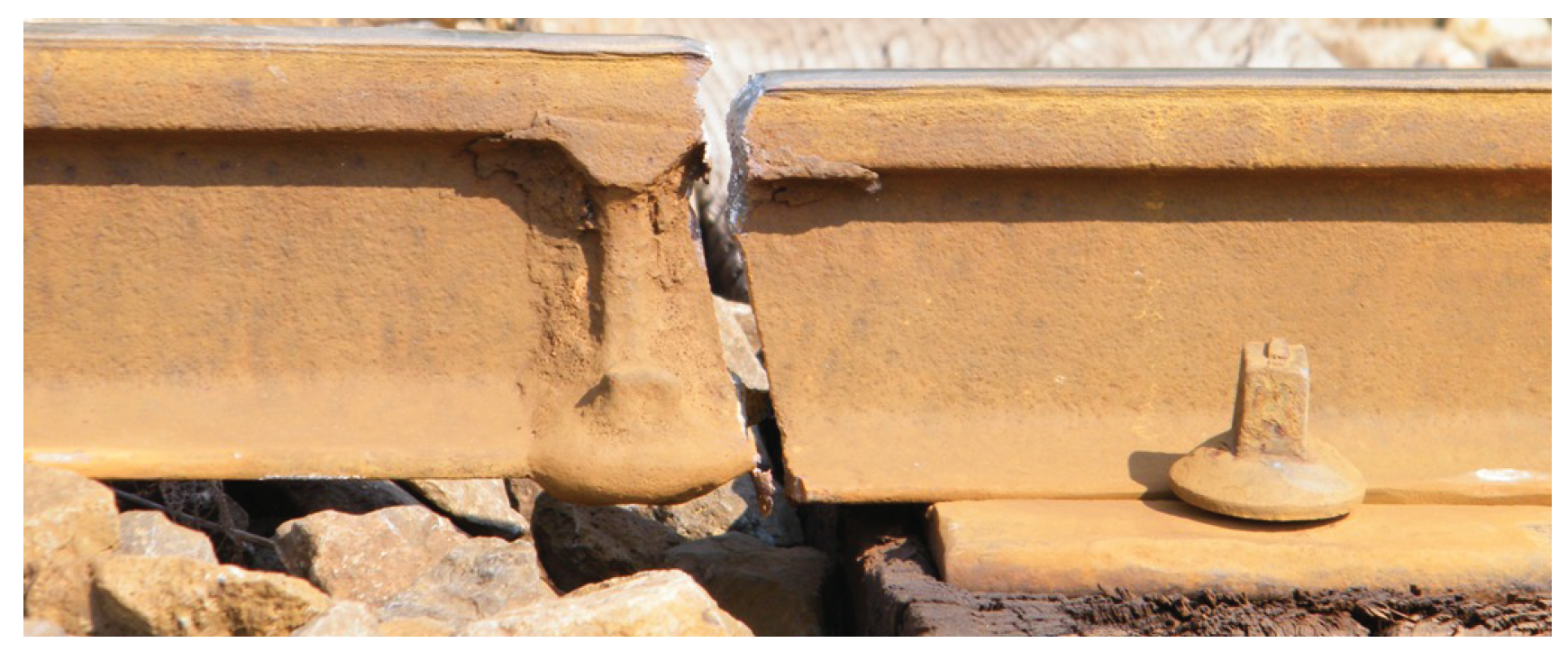
2.3. Rail Joints
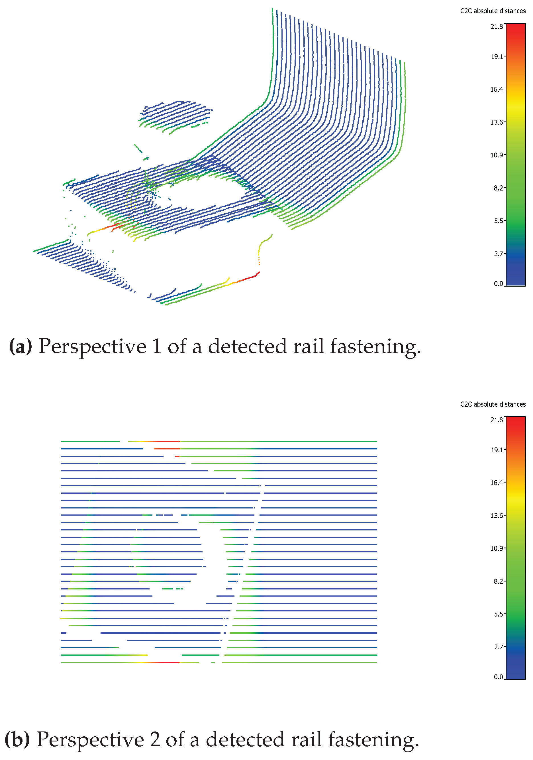
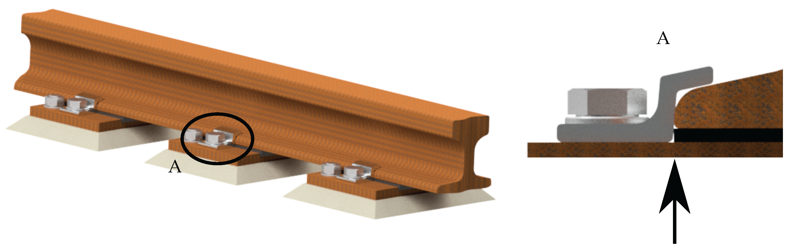
2.4. Rail Fastenings
2.5. Measurement in the Loaded and Unloaded State
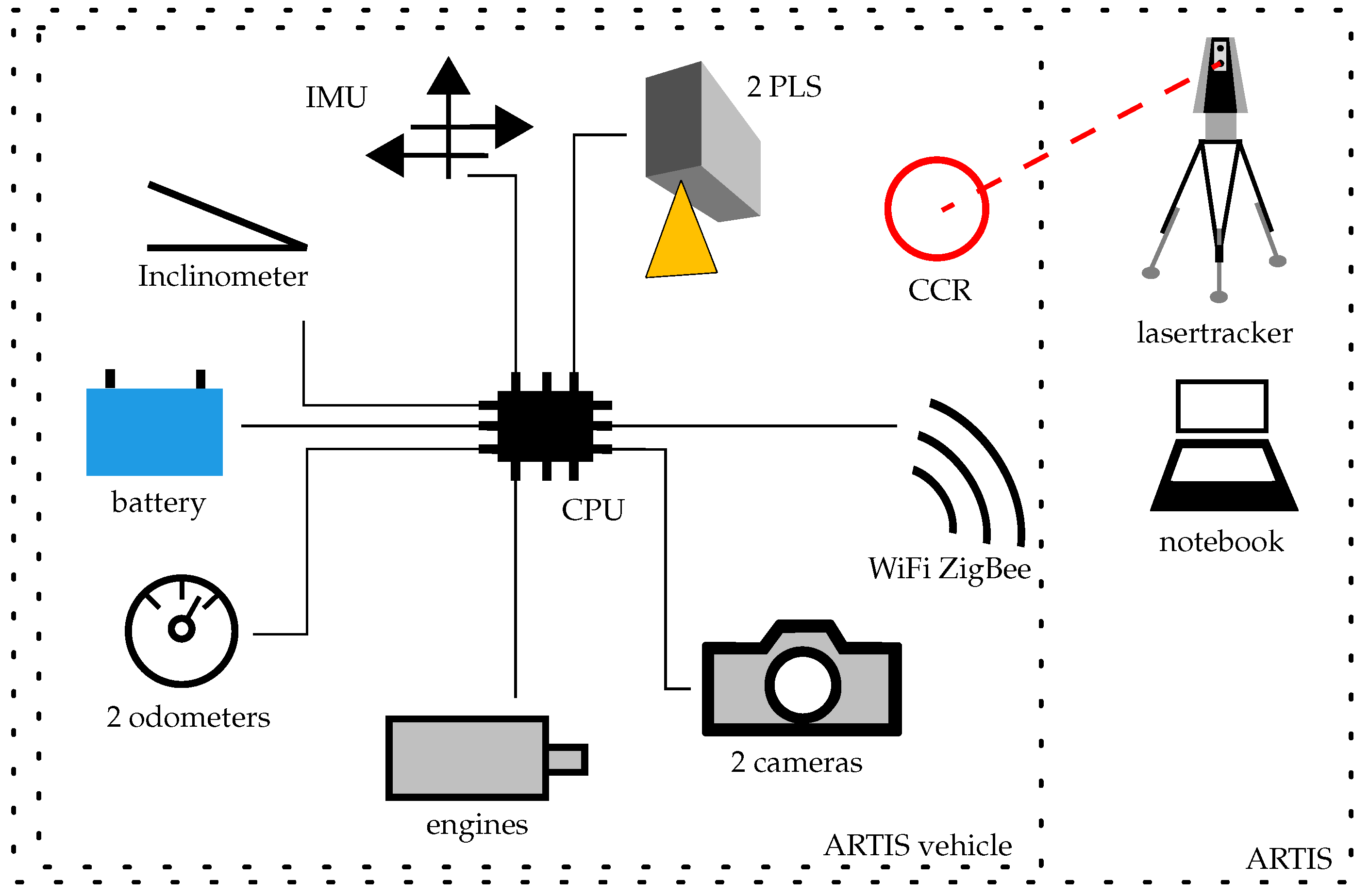
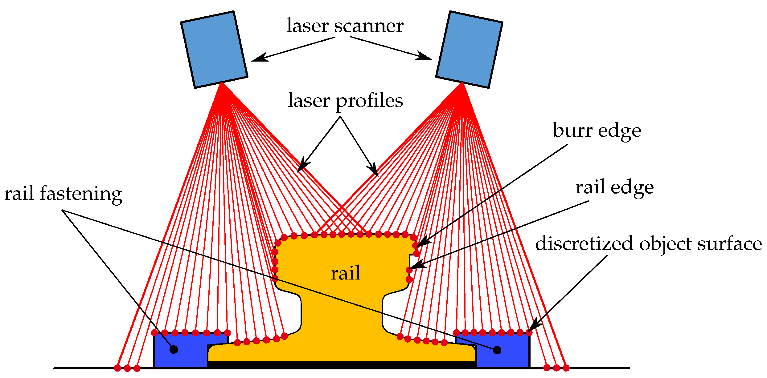
3. Concept and Realization
- 2 profile laser scanner (PLS)
- 2 cameras
- 1 inertial measuring unit (IMU)
- 1 inclinometer
- 2 odometer
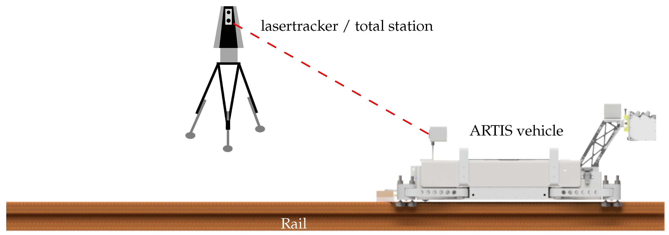
- When the target values, defined by existing standards, are determined, the vehicle platform (without PLS and cameras) is tracked by means of a total station or a lasertracker. For this purpose, a corner cube retroreflector (CCR) is attached to the vehicle.
- For documentation of the condition of the rail, of the rail fastening and the rail inclination, the vehicle platform is equipped with PLS and cameras and the travelled distance is determined by means of the odometers. A total station or lasertracker is not used.
4. Measurement Uncertainty of the Target Variables and Requirements for the Sensor Technology
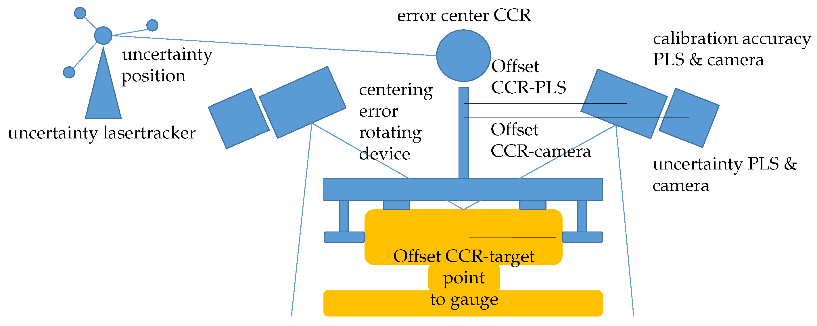
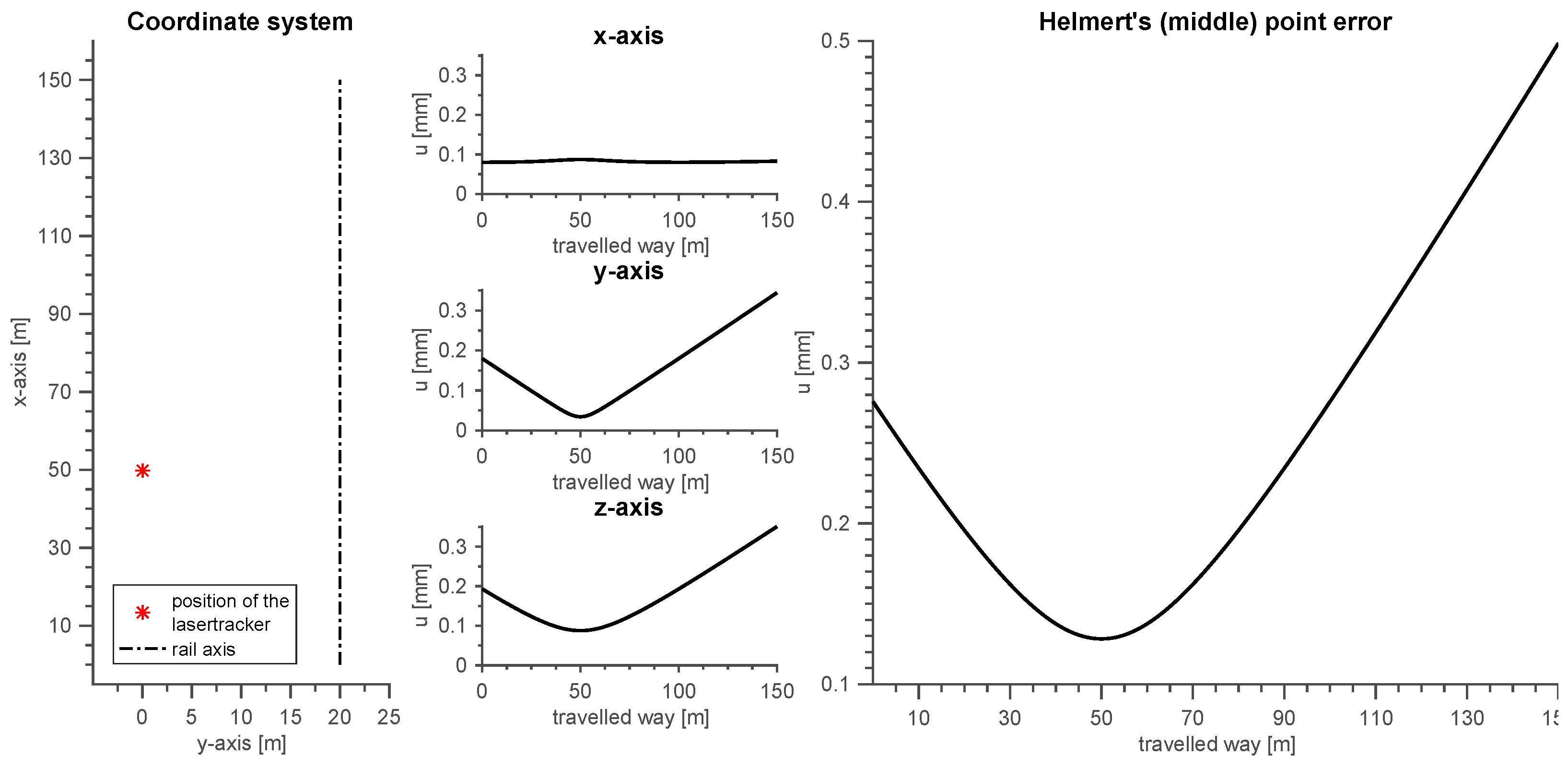
4.1. Measurement Uncertainty of the Position of the ARTIS Vehicle
4.2. Measurement Uncertainty of the Burr Width at the Rail Head
5. Hardware and Software
5.1. Hardware
5.2. Electronic Components
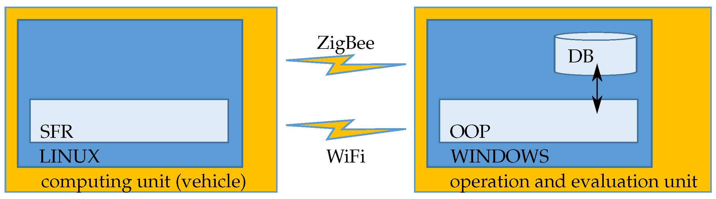
5.3. Implementation
5.4. Software
6. Calibration of the PLS
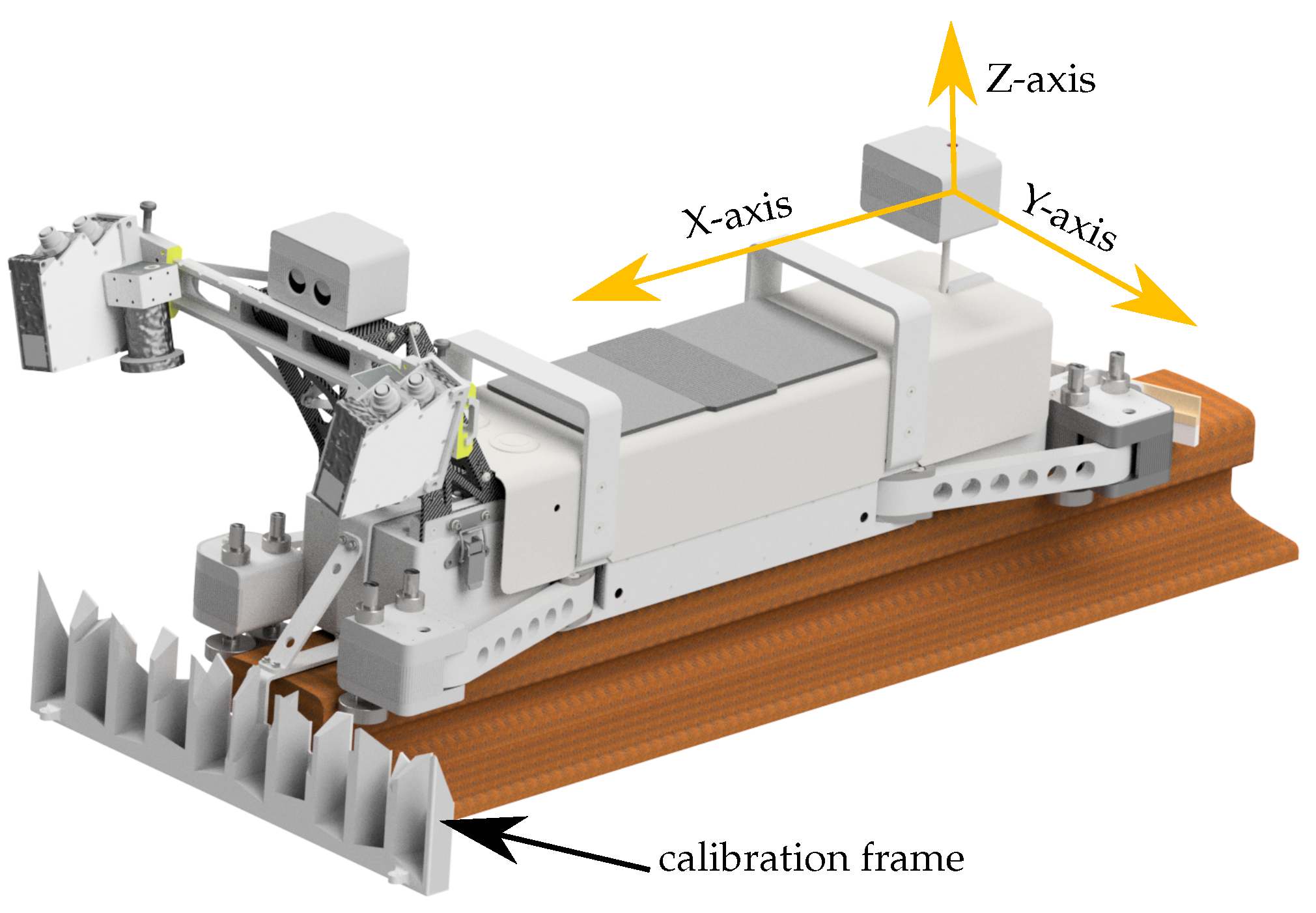
6.1. Superior Vehicle Coordinate System
6.2. Basic Idea
6.3. Calibration Frame
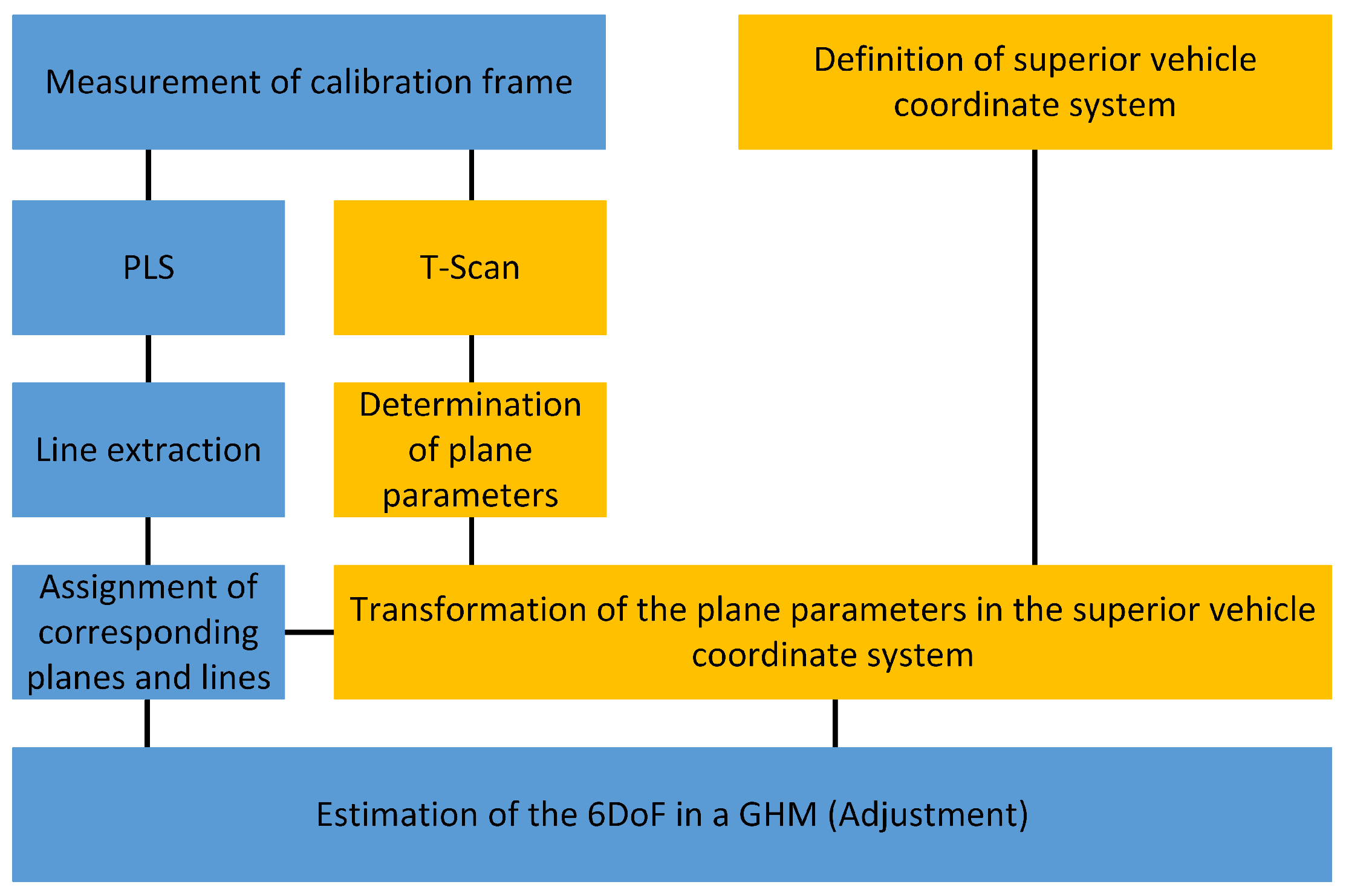
6.4. Workflow
7. Results
8. Conclusions
Acknowledgments

Author Contributions
Conflicts of Interest
Abbreviations
| ARTIS | Advanced Railtrack Inspection System |
| CAD | Computer-aided design |
| CCD | Charge-coupled device |
| CCR | Corner cube retroreflector |
| CPU | Central processing unit |
| CTSS | Crane track surveying system |
| DB | Database |
| GHM | Gauss-Helmert model |
| GUM | Guide to the Expression of Uncertainty in Measurement |
| IMU | Inertial measurement unit |
| ISO | International Organization for Standardization |
| lre | Left rail edge |
| MEMS | Microelectromechanical system |
| OOP | Object-oriented programming |
| PLS | Profile laser scanner |
| rre | Right rail edge |
| 6DoF | Six degrees of freedom |
| SFR | Software framework for robots |
| USB | Universal serial bus |
| VCS | Vehicle coordinate system |
| wlre | Worn left rail edge |
| wrre | Worn right rail edge |
References
- ISO. ISO 12488-1 Cranes—Tolerances for Wheels and Travel and Traversing Tracks—Part 1: General; ISO: Geneva, Switzerland, 2012. [Google Scholar]
- Tlustý, J. Anwendung von Lasergeräten für die Vermessung von Kranbahnen. Vermessungstechnik 1979, 27, 129–130. [Google Scholar]
- Hánek, P.; Buršíková, O. Měření jeřábových drah totálními stanicemi. Geodetický a kartografický 1993, 39, 8–11. [Google Scholar]
- Marjetič, A.; Kregar, K.; Ambrožič, T.; Kogoj, D. An Alternative Approach to Control Measurements of Crane Rails. Sensors 2012, 12, 5906–5918. [Google Scholar] [CrossRef] [PubMed]
- Neumann, I.; Dennig, D. Development of the kinematic Crane-Track-Surveying-System “RailControl”. AVN 2012, 5, 162–169. [Google Scholar]
- Möser, M. Krane und Kranbahnen. In Ingenieurbau; Wichmann Verlag: Berlin, Germany, 2016; pp. 169–188. [Google Scholar]
- Mao, J.; Nindl, D. Surveying Reflectors—White Paper: Characteristics and Influences. Leica Geosystems, 2009. Available online: http://accessories.leica-geosystems.com/downloads123/zz/accessory/accessories/white-tech-paper/WhitePaperSurveyingReflectors_en.pdf (accessed on 18 January 2017).
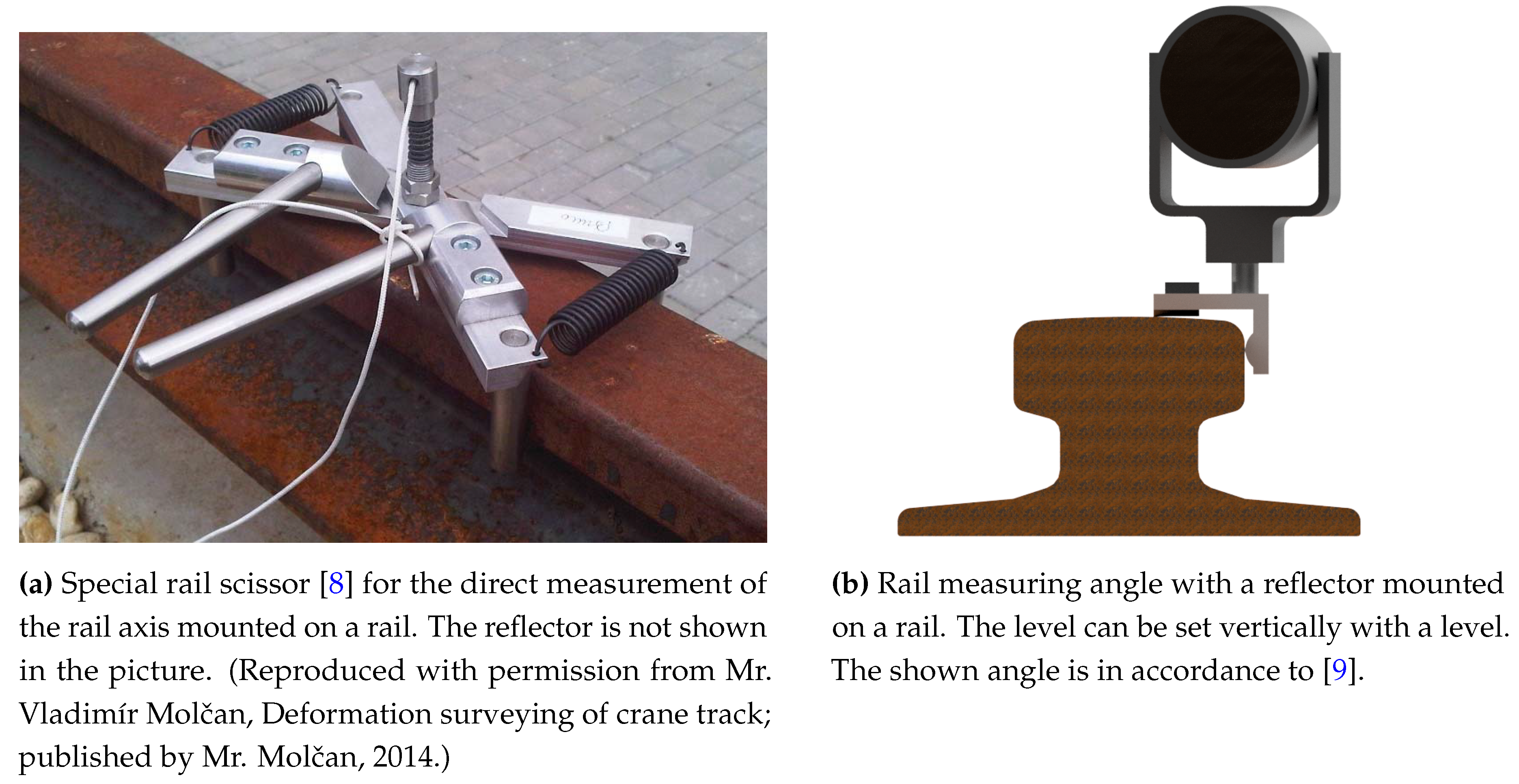
- Molčan, V. Deformation Surveying of Crane Track. Master’s Thesis, Brno University of Technology, Brno, Czech Republic, 2014. [Google Scholar]
- Goecke GmbH & Co. KG. Available online: http://goecke.de/Products/Railway-survey-equipment/Universal-prisms-for-railway-surveying/Magnetic-track-measuring-angle.html (accessed on 21 February 2017).
- Wikipedia. Rail Inspection. Available online: https://en.wikipedia.org/wiki/Rail_inspection (accessed on 26 January 2017).
- JCGM 100:2008. GUM 1995 with Minor Corrections. Evaluation of Measurement Data—Guide to the Expression of Uncertainty in Measurement (GUM); ISO: Geneva, Switzerland, 2008. [Google Scholar]
- DIN. DIN 18710-1 Engineering Survey—Part 1: General Requirements; DIN: Berlin, Germany, 2011. [Google Scholar]
- Fontana, R.; Gambino, M.; Grecoa, M.; Pampaloni, E.; Pezzati, L.; Scopigno, R. High-resolution 3D digital models of artworks. Proc. SPIE 2003, 5146, 34–43. [Google Scholar]
- Strübing, T.; Neumann, I. Positions- und Orientierungsschätzung von LIDAR-Sensoren auf Multisensorplattformen. ZfV 2013, 3, 210–221. [Google Scholar]
- Schaffrin, B.; Wieser, A. On weighted total least-squares adjustment for linear regression. J. Geod. 2008, 7, 415–421. [Google Scholar] [CrossRef]
- Hartmann, J.; Paffenholz, J.-A.; Strübing, T.; Neumann, I. Determination of position and orientation of lidar-sensors of multi-sensor platforms. J. Surv. Eng. 2017, 4, 04017012. [Google Scholar] [CrossRef]
- Leica Geosystems AG. Available online: http://metrology.leica-geosystems.com/en/Leica-T-Scan_1836.htm?changelang=true (accessed on 11 April 2017).


| Target Value | Coordinate | Reference | Accuracy | Sensors |
|---|---|---|---|---|
| position of the rails | X, Y | absolute | submillimeter | lasertracker, optional PLS |
| height of the rails | X, Z | |||
| position and height of adjacent rails | X, Y, Z | |||
| longitudinal inclination of the rail head | X, Z | absolute | <0.06° | lasertracker, inclinometer |
| lateral inclination of the rail head | Y, Z | <0.01° | ||
| practical and theoretical rail axes | X, Y, Z | absolute | submillimeter | lasertracker, PLS |
| breaking out in the rail head | X, Y, Z | absolute, relative | centimeter (X), submillimeter (Y, Z) | lasertracker or odometer, PLS, camera |
| wheel slip marks | ||||
| burr on the rail head | ||||
| long and transverse cracks in the rail head | ||||
| rail height | X, Z | absolute, relative | centimeter (X), submillimeter (Z) | lasertracker or odometer, PLS |
| position of rail fastenings | X | absolute | millimeter | lasertracker or odometer, PLS, camera |
| condition of rail fastenings | ||||
| position of the rail joint | lasertracker or odometer, PLS, camera, IMU | |||
| type of a rail joint |
| Influencing Value | Uncertainty | Type | |
|---|---|---|---|
| Y component of the position of the lasertracker | A | ||
| z | zenith / elevation angle | B | |
| slope distance | B | ||
| t | azimuth | B | |
| Y component offset target point to gauge line | A | ||
| centering error rotating device | A | ||
| CCR error center | B | ||
| CCR error spherical shape | B | ||
| Z component offset CCR-top of rail | A | ||
| in | inclination from inclinometer | B | |
| Influencing Value | Uncertainty | Type | |
|---|---|---|---|
| edge burr | B | ||
| edge rail | |||
© 2017 by the authors. Licensee MDPI, Basel, Switzerland. This article is an open access article distributed under the terms and conditions of the Creative Commons Attribution (CC BY) license (http://creativecommons.org/licenses/by/4.0/).
Share and Cite
Dennig, D.; Bureick, J.; Link, J.; Diener, D.; Hesse, C.; Neumann, I. Comprehensive and Highly Accurate Measurements of Crane Runways, Profiles and Fastenings. Sensors 2017, 17, 1118. https://doi.org/10.3390/s17051118
Dennig D, Bureick J, Link J, Diener D, Hesse C, Neumann I. Comprehensive and Highly Accurate Measurements of Crane Runways, Profiles and Fastenings. Sensors. 2017; 17(5):1118. https://doi.org/10.3390/s17051118
Chicago/Turabian StyleDennig, Dirk, Johannes Bureick, Johannes Link, Dmitri Diener, Christian Hesse, and Ingo Neumann. 2017. "Comprehensive and Highly Accurate Measurements of Crane Runways, Profiles and Fastenings" Sensors 17, no. 5: 1118. https://doi.org/10.3390/s17051118
APA StyleDennig, D., Bureick, J., Link, J., Diener, D., Hesse, C., & Neumann, I. (2017). Comprehensive and Highly Accurate Measurements of Crane Runways, Profiles and Fastenings. Sensors, 17(5), 1118. https://doi.org/10.3390/s17051118