Robust In-Flight Sensor Fault Diagnostics for Aircraft Engine Based on Sliding Mode Observers


Abstract
:1. Introduction
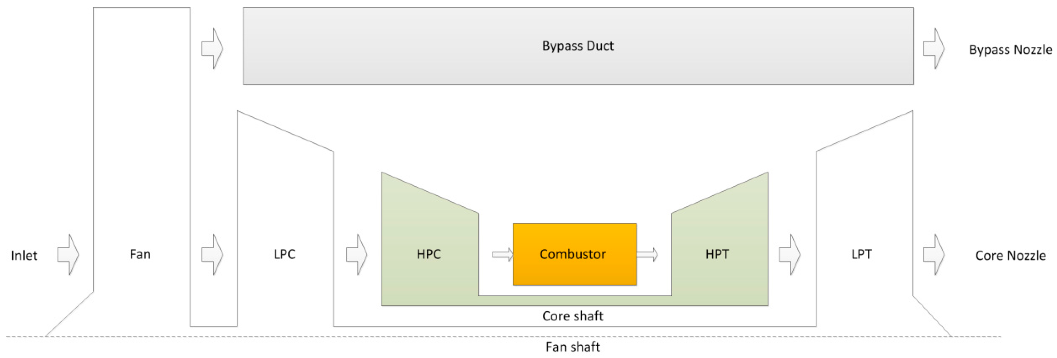
2. Aircraft Engine Description
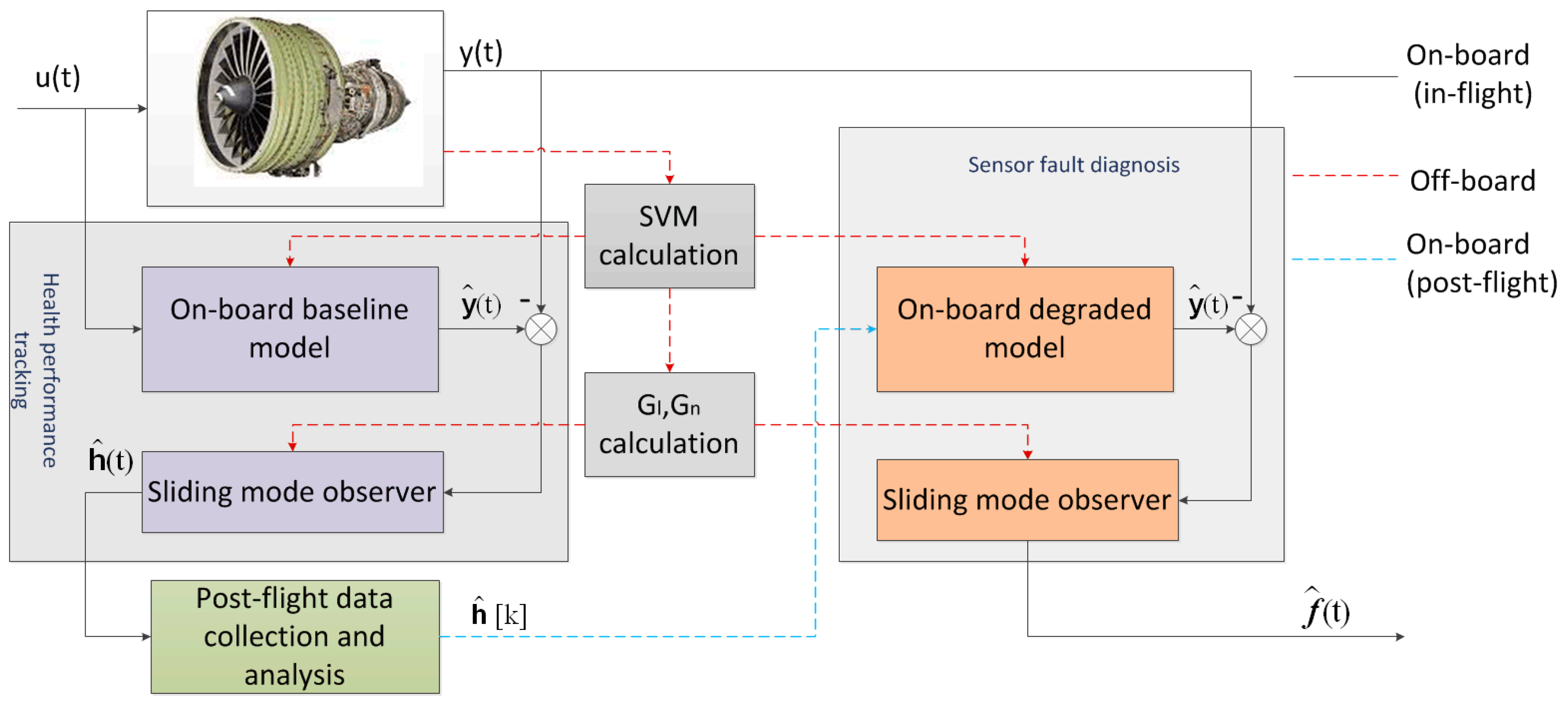
3. Sensor Fault Diagnostic
- The first Markov parameter (the product of and ) must have full column rank;
- Any invariant zeroes (if there exists) of are Hurwitz.
4. Degraded Performance Tracking and Post-Flight Model Update
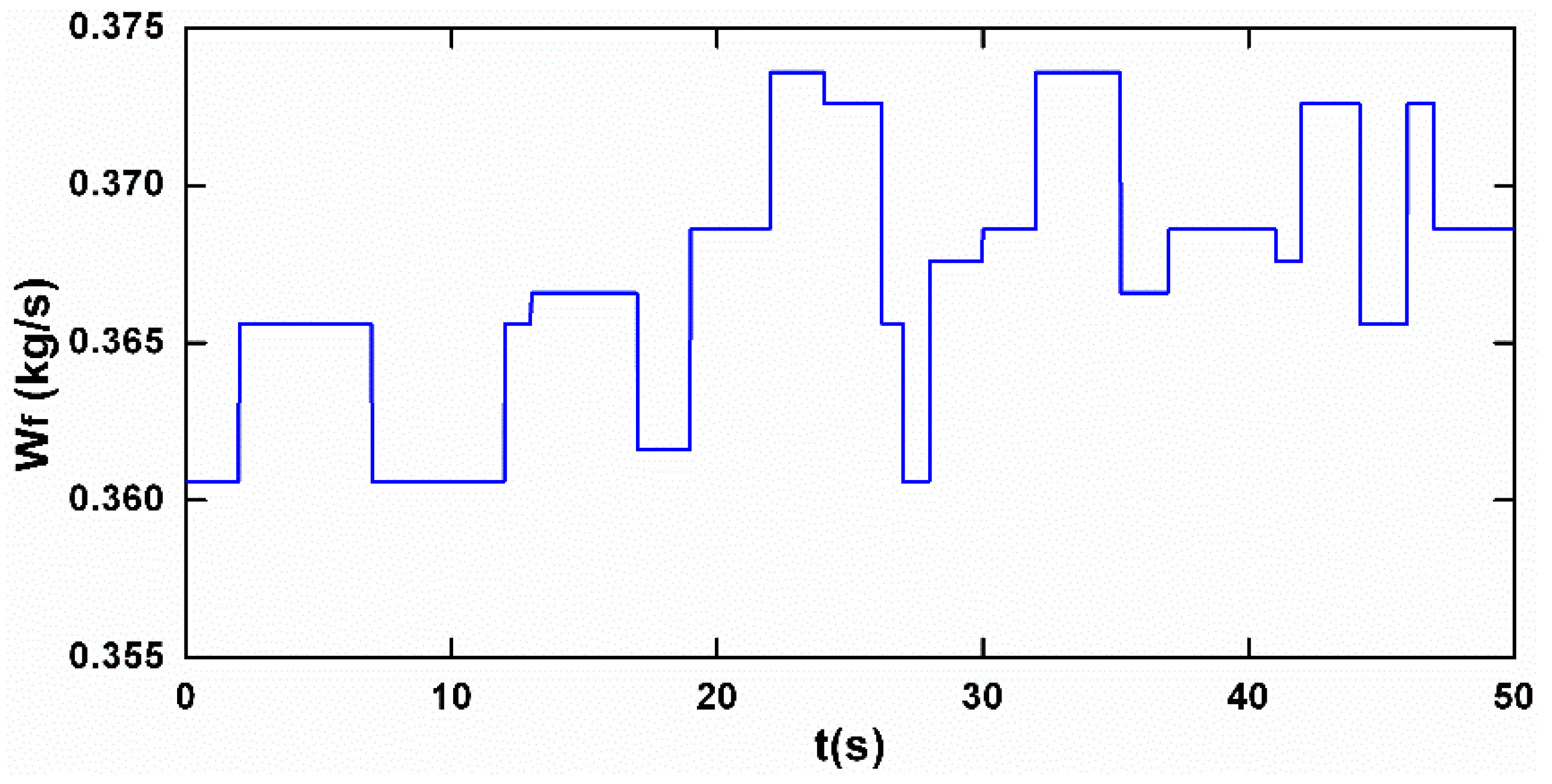
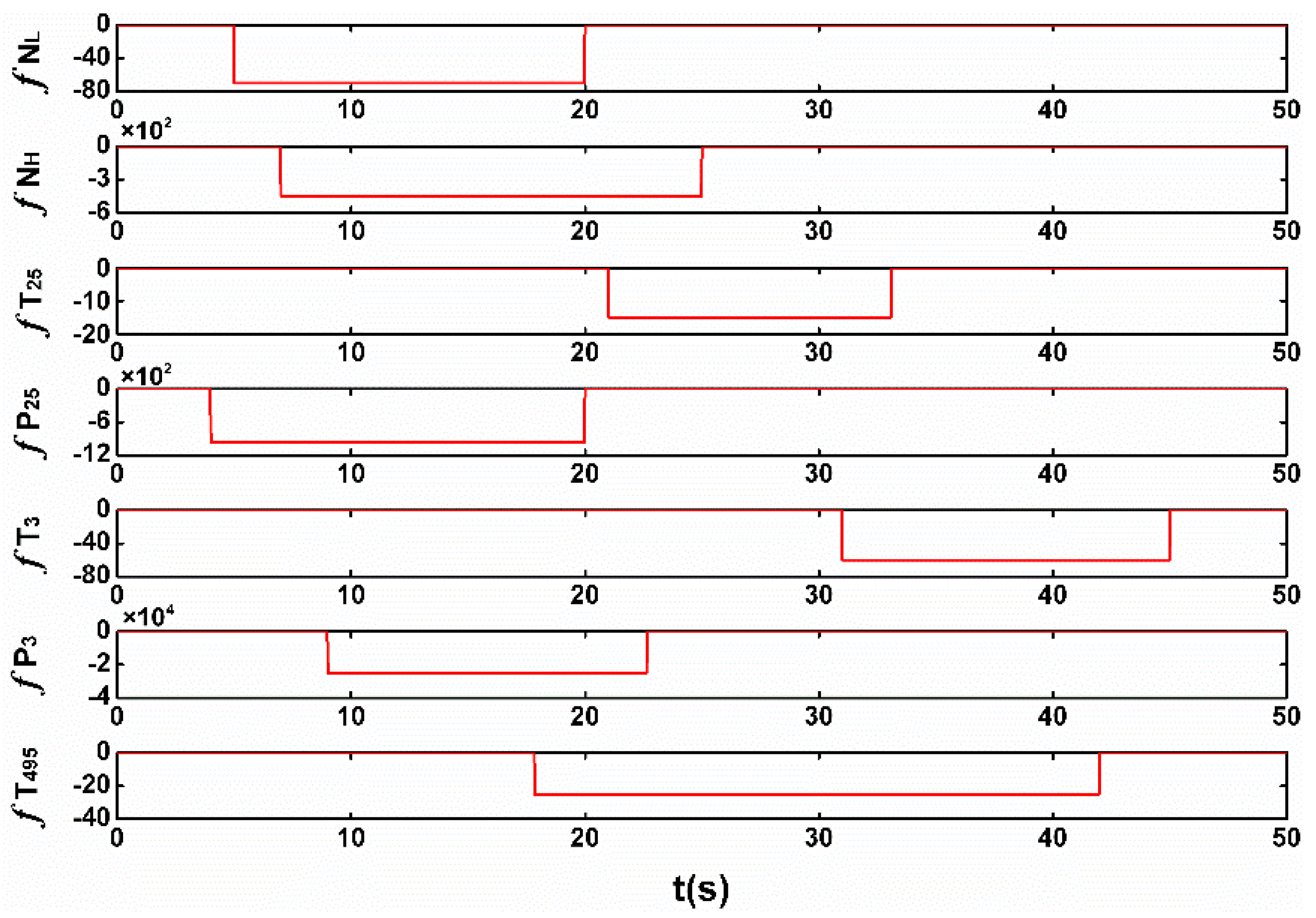
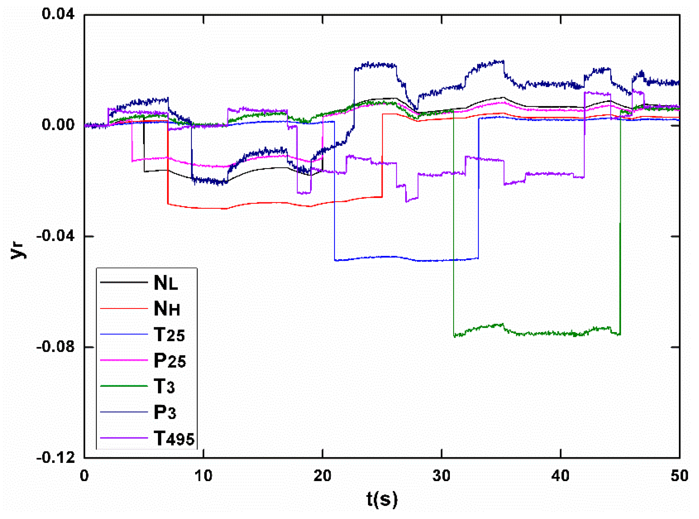
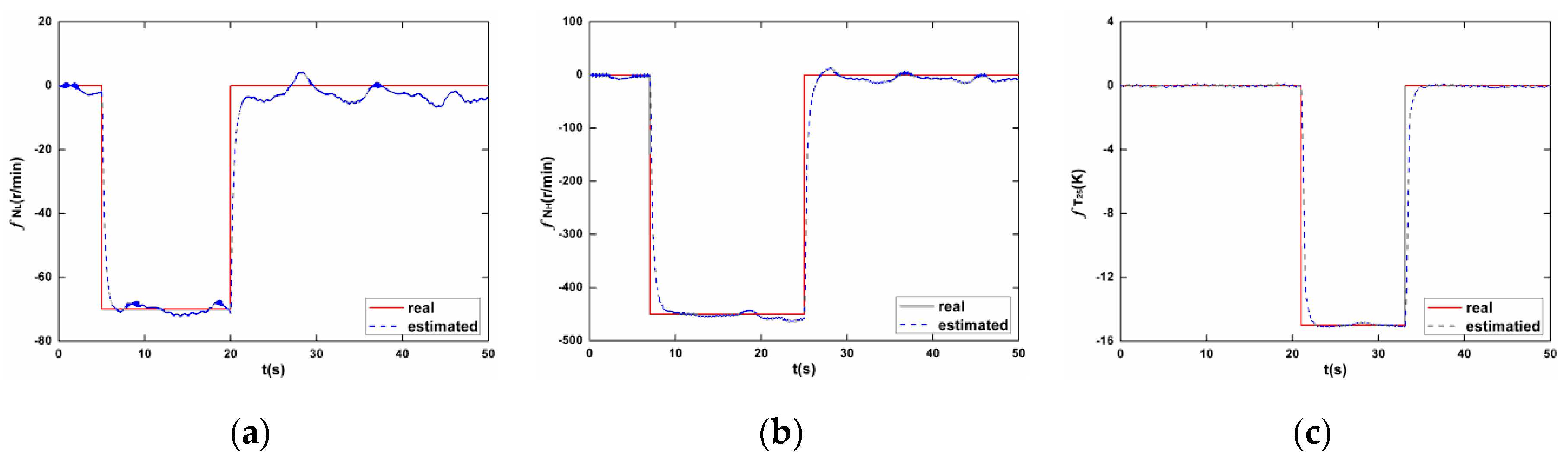
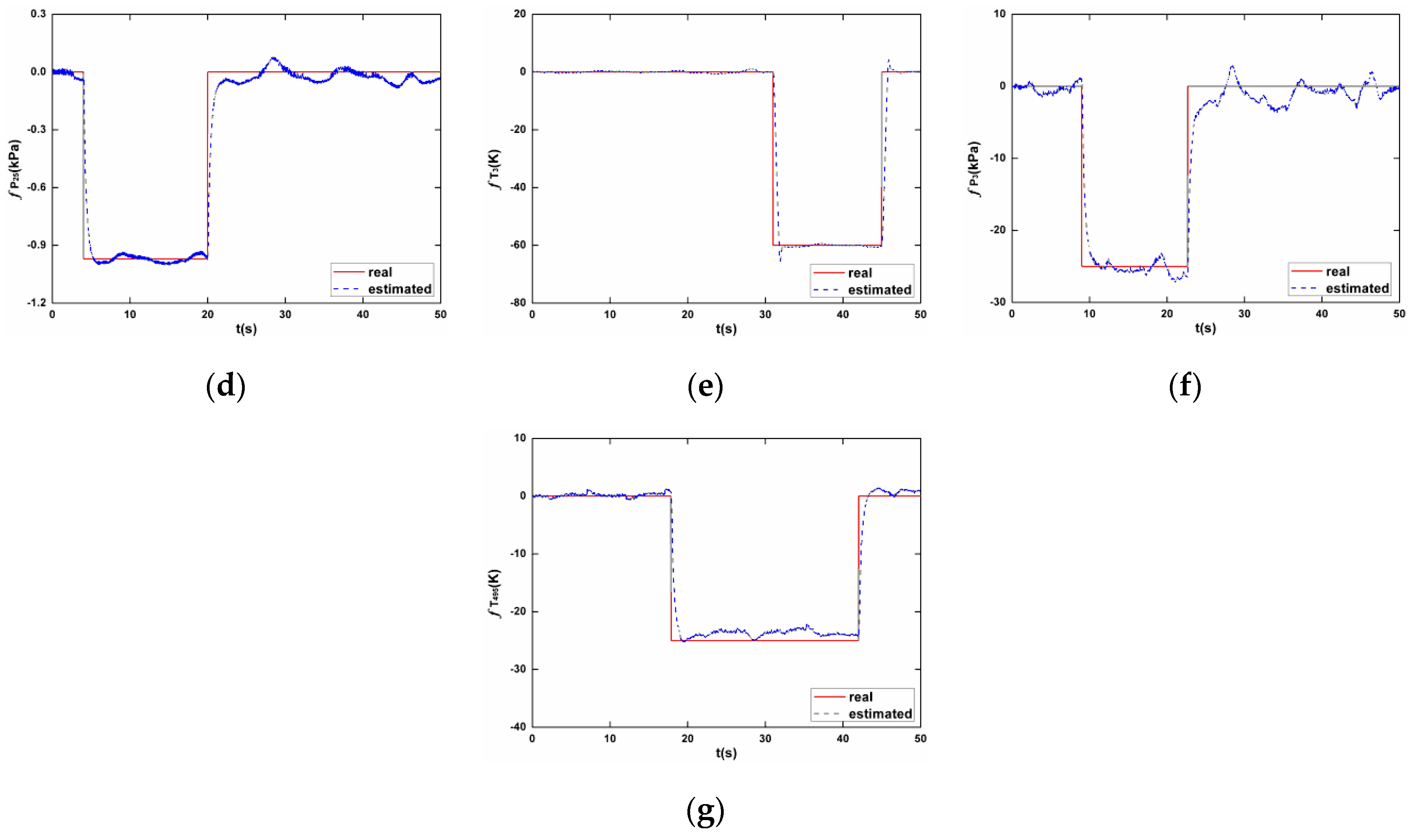
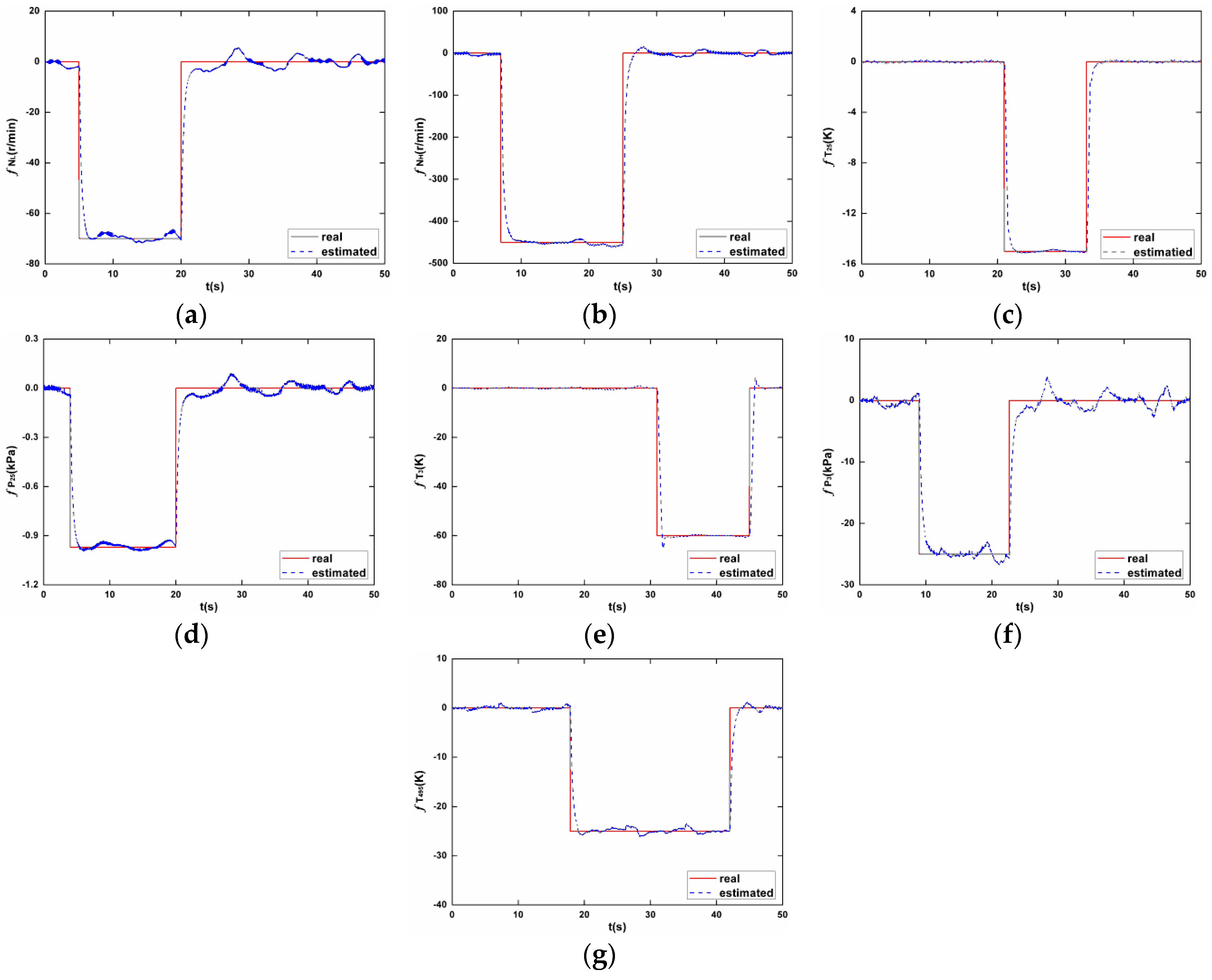
5. Simulation and Performance Evaluation
6. Conclusions
Acknowledgments
Author Contributions
Conflicts of Interest
References
- Merrill, W.C.; Delaat, J.C.; Bruton, W.M. Advanced detection, isolation, and accommodation of sensor failures—Real-time evaluation. J. Guid. Control Dynam. 1988, 11, 517–526. [Google Scholar] [CrossRef]
- Kobayashi, T.; Simon, D.L. Evaluation of an enhanced bank of Kalman filters for in-flight aircraft engine sensor fault diagnostics. J. Eng. Gas Turbines Power 2005, 127, 497–504. [Google Scholar] [CrossRef]
- Simon, D.L. An Integrated Architecture for on-Board Aircraft Engine Performance Trend Monitoring and Gas Path Fault Diagnostics; Technical Report; NASA Glenn Research Center: Cleveland, OH, USA, 2010.
- Armstrong, J.B.; Simon, D.L. Implementation of an integrated on-board aircraft engine diagnostic architecture. In Proceedings of the 47th Joint Propulsion Conference and Exhibit, San Diego, CA, USA, 31 July–3 August 2011. [Google Scholar]
- Kobayashi, T.; Simon, D.L. Hybrid Kalman Filter: A New Approach for Aircraft Engine In-flight Diagnostics; Technical Report; NASA Glenn Research Center: Cleveland, OH, USA, 2006.
- Tan, C.P.; Edwards, C. A robust sensor fault reconstruction scheme using sliding mode observers applied to a nonlinear aero-engine model. In Proceedings of the American Control Conference, IEEE, Anchorage, AK, USA, 8–10 May 2002. [Google Scholar]
- Alwi, H.; Edwards, C. Development and application of sliding mode LPV fault reconstruction schemes for the ADDSAFE Benchmark. Control Eng. Pract. 2014, 31, 148–170. [Google Scholar] [CrossRef]
- Rahme, S.; Meskin, N. Adaptive sliding mode observer for sensor fault diagnosis of an industrial gas turbine. Control Eng. Pract. 2015, 38, 57–74. [Google Scholar] [CrossRef]
- Chang, X.; Huang, J.; Lu, F.; Sun, H. Gas-path Health Estimation for an Aircraft Engine Based on a Sliding mode observer. Energies 2016, 9, 598. [Google Scholar] [CrossRef]
- Edwards, C.; Spurgeon, S.K. Sliding Mode Control: Theory and Applications; CRC Press: Boca Raton, FL, USA, 1988. [Google Scholar]
- Alwi, H.; Edwards, C. Robust fault reconstruction for linear parameter varying systems using sliding mode observers. Int. J. Robust Nonlinear Control 2013, 24, 1947–1968. [Google Scholar] [CrossRef]
- Moreno, J.A.; Osorio, M. Strict Lyapunov Functions for the Super-Twisting Algorithm. IEEE Trans. Autom. Control 2012, 57, 1035–1040. [Google Scholar] [CrossRef]
- Edwards, C.; Alwi, H.; Tan, C.P. Sliding Modes for Fault Detection and Fault-Tolerant Control. In Sliding Modes after the First Decade of the 21st Century; Springer: Berlin, Germany, 2012; pp. 293–323. [Google Scholar]
- Lu, F.; Huang, J.; Lv, Y. Gas Path Health Monitoring for a Turbofan Engine Based on a Nonlinear Filtering Approach. Energies 2013, 6, 492–513. [Google Scholar] [CrossRef]
- Zhou, W.X. Research on Object-Oriented Modeling and Simulation for Aeroengine and Control System. Ph.D. Thesis, Nanjing University of Aeronautics and Astronautics, Nanjing, China, 2006. (In Chinese). [Google Scholar]
- Lu, F.; Huang, J. Engine Component Performance Prognostics based on Decision Fusion. Acta Aeronaut. Astronaut. Sin. 2009, 30, 1795–1800. [Google Scholar]


| Notation | Description |
|---|---|
| H | Height |
| Ma | Mach number |
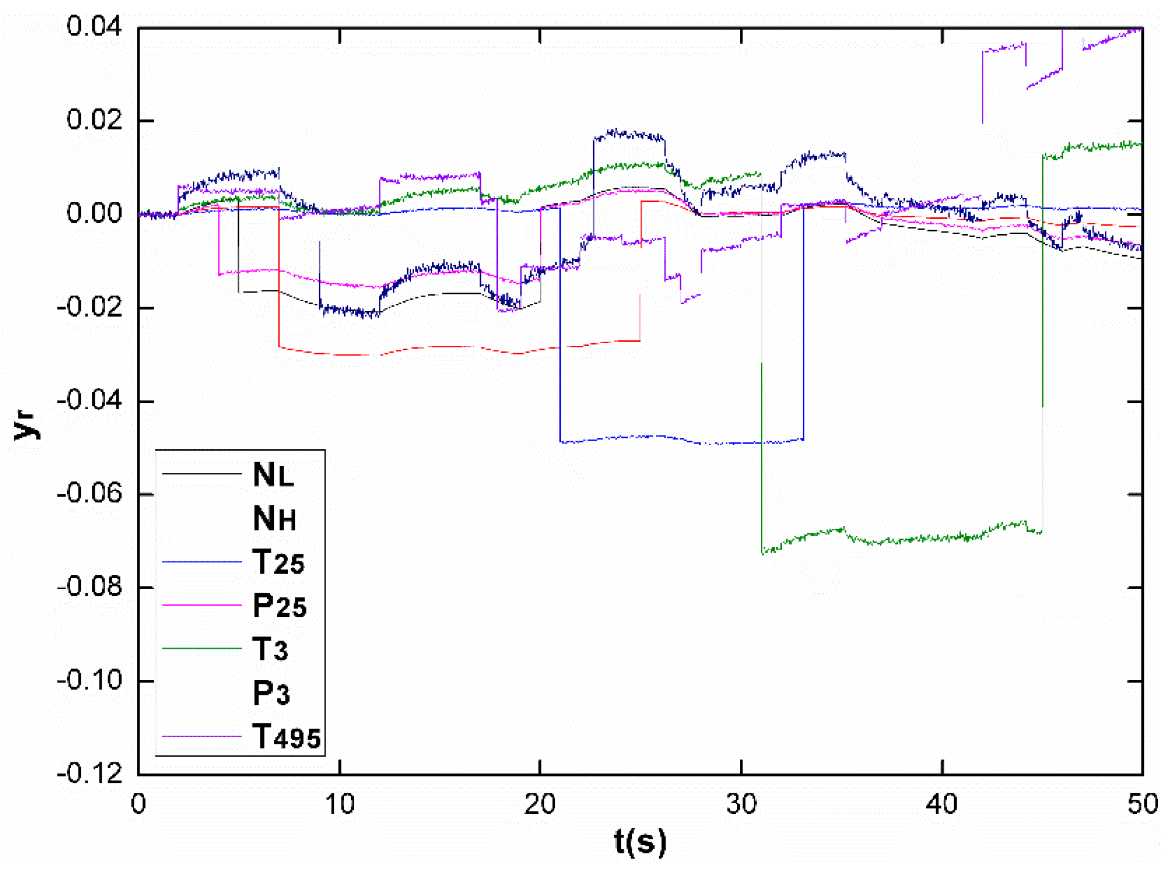
| NL | Low pressure rotor speed |
| NH | High pressure rotor speed |
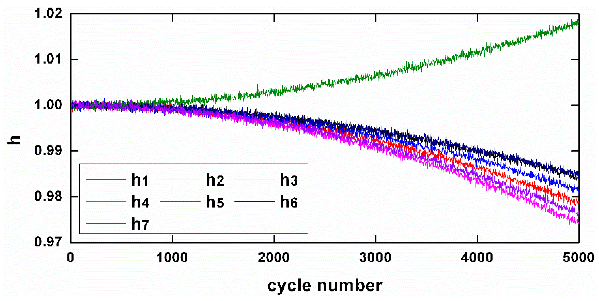
| h | Health parameter vector |
| h1 | LPC efficiency |
| h2 | HPC efficiency |
| h3 | HPT efficiency |
| h4 | LPT efficiency |
| h5 | LPC flow capacity |
| h6 | HPC flow capacity |
| h7 | HPT flow capacity |
| h8 | LPT flow capacity |
| Wf | Fuel flow rate |
| P25 | HPC inlet pressure |
| T25 | HPC inlet temperature |
| P3 | Combustor inlet pressure |
| T3 | Combustor inlet temperature |
| T495 | Exhaust gas temperature |
| Measurement | Nominal Value | Fault Magnitude |
|---|---|---|
| 3484 RPM | −2% | |
| 15,044 RPM | −3% | |
| 298 K | −5% | |
| 64,990 Pa | −1.5% | |
| 747 K | −8% | |
| 1,242,145 Pa | −2% | |
| 936 K | −2.5% |
| Non-Degrading Case | Degrading Case | |
|---|---|---|
| 0.197 | 0.208 | |
| 0.294 | 0.298 | |
| 0.515 | 0.516 | |
| 0.143 | 0.146 | |
| 0.895 | 0.895 | |
| 0.219 | 0.236 | |
| 0.241 | 0.252 |
© 2017 by the authors. Licensee MDPI, Basel, Switzerland. This article is an open access article distributed under the terms and conditions of the Creative Commons Attribution (CC BY) license (http://creativecommons.org/licenses/by/4.0/).
Share and Cite
Chang, X.; Huang, J.; Lu, F. Robust In-Flight Sensor Fault Diagnostics for Aircraft Engine Based on Sliding Mode Observers. Sensors 2017, 17, 835. https://doi.org/10.3390/s17040835
Chang X, Huang J, Lu F. Robust In-Flight Sensor Fault Diagnostics for Aircraft Engine Based on Sliding Mode Observers. Sensors. 2017; 17(4):835. https://doi.org/10.3390/s17040835
Chicago/Turabian StyleChang, Xiaodong, Jinquan Huang, and Feng Lu. 2017. "Robust In-Flight Sensor Fault Diagnostics for Aircraft Engine Based on Sliding Mode Observers" Sensors 17, no. 4: 835. https://doi.org/10.3390/s17040835
APA StyleChang, X., Huang, J., & Lu, F. (2017). Robust In-Flight Sensor Fault Diagnostics for Aircraft Engine Based on Sliding Mode Observers. Sensors, 17(4), 835. https://doi.org/10.3390/s17040835