Hazards in Motion: Development of Mobile Geofences for Use in Logging Safety


Abstract
:1. Introduction
2. Materials and Methods
3. Results
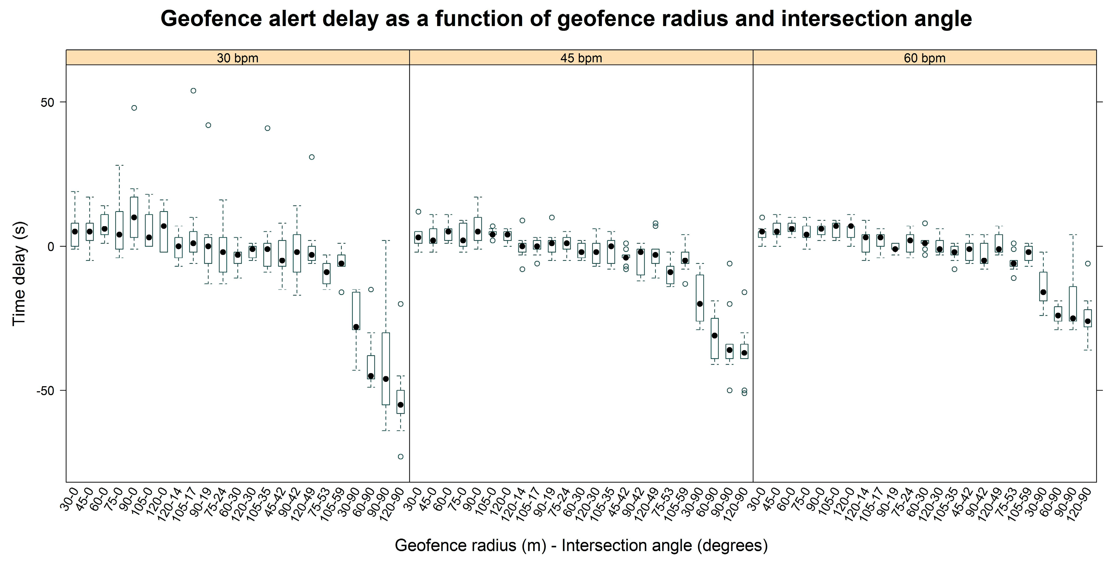
3.1. Field Results
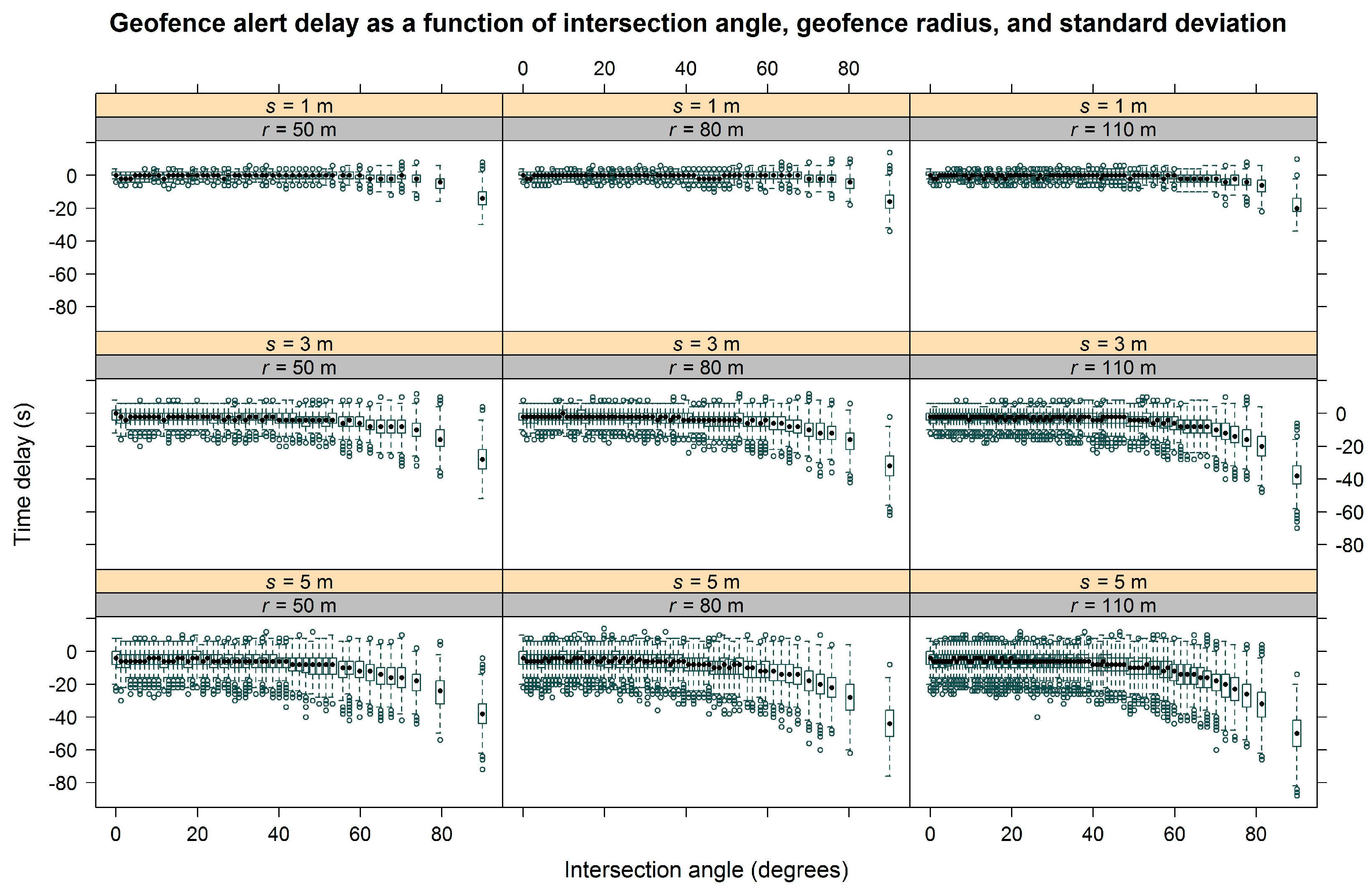
3.2. Simulation Results
4. Discussion
5. Conclusions
Acknowledgments
Author Contributions
Conflicts of Interest
References
- Sygnatur, E.F. Logging is perilous work. Compens. Work. Cond. 1998, 3, 3–9. [Google Scholar]
- Fosbroke, D.E.; Kisner, S.M.; Myers, J.R. Working lifetime risk of occupational fatal injury. Am. J. Ind. Med. 1997, 31, 459–467. [Google Scholar] [CrossRef]
- Sullman, M.J.M.; Kirk, P.M.; Parker, R.J.; Gaskin, J.E. New Zealand logging industry accident reporting scheme: Focus for a human factors research programme. J. Saf. Res. 1999, 30, 123–131. [Google Scholar] [CrossRef]
- Wang, J.; Bell, J.L.; Grushecky, S.T. Logging injuries for a 10-year period in Jilin Province of the People’s Republic of China. J. Saf. Res. 2003, 34, 273–279. [Google Scholar] [CrossRef]
- Axelsson, S.A. The mechanization of logging operations in Sweden and its effect on occupational safety and health. J. For. Eng. 1998, 9, 25–31. [Google Scholar]
- Bell, J.L. Changes in logging injury rates associated with use of feller-bunchers in West Virginia. J. Saf. Res. 2002, 33, 463–471. [Google Scholar] [CrossRef]
- Egan, A.F. The introduction of a comprehensive logging safety standard in the USA—The first eighteen months. J. For. Eng. 1998, 9, 17–23. [Google Scholar]
- Bordas, R.M.; Davis, G.A.; Hopkins, B.L.; Thomas, R.E.; Rummer, R.B. Documentation of hazards and safety perceptions for mechanized logging operations in East Central Alabama. J. Agric. Saf. Health 2001, 7, 113–123. [Google Scholar] [CrossRef] [PubMed]
- U.S. Bureau of Labor Statistics. Current Population Survey, Census of Fatal Occupational Injuries. 2016. Available online: http://www.bls.gov/iif/oshcfoi1.htm (accessed on 15 January 2017).
- Keefe, R.F.; Eitel, J.U.H. Applications of carriage-mounted agricultural cameras to improve safety in cable logging operations. In Proceedings of the 2013 Annual Meeting of the Council on Forest Engineering, Missoula, MT, USA, 7–10 July 2013. [Google Scholar]
- Wing, M.G.; Eklund, A.; Kellogg, L.D. Consumer-grade global positioning system (GPS) accuracy and reliability. J. For. 2005, 103, 169–173. [Google Scholar]
- Johnson, C.E.; Barton, C.C. Where in the world are my field plots? Using GPS effectively in environmental field studies. Front. Ecol. Environ. 2004, 2, 475–482. [Google Scholar] [CrossRef]
- Bettinger, P.; Fei, S. One year’s experience with a recreation-grade GPS receiver. Math. Comput. For. Nat. Resour. Sci. 2010, 2, 153–160. [Google Scholar]
- Wing, M.G. Consumer-grade global positioning systems (GPS) receiver performance. J. For. 2008, 106, 185–190. [Google Scholar]
- Wing, M.G. Consumer-grade GPS receiver measurement accuracy in varying forest conditions. Res. J. For. 2011, 5, 78–88. [Google Scholar] [CrossRef]
- Andersen, H.E.; Clarkin, T.; Winterberger, K.; Strunk, J. An accuracy assessment of positions obtained using survey- and recreational-grade global positioning system receivers across a range of forest conditions within the Tanana Valley of interior Alaska. West. J. Appl. For. 2009, 24, 128–136. [Google Scholar]
- Reclus, F. Geofencing. In Geopositioning and Mobility; Nait-Sidi-Moh, A., Bakhouya, M., Gaber, J., Wack, M., Eds.; Johny Wiley & Sons, Inc.: Hoboken, NJ, USA, 2013; pp. 127–154. [Google Scholar]
- Namiot, D. GeoFence services. Int. J. Open Inf. Technol. 2013, 1, 30–33. [Google Scholar]
- Reclus, F.; Drouard, K. Geofencing for fleet & freight management. In Proceedings of the 9th International Conference on Intelligent Transport Systems Telecommunications (ITST), Lille, France, 20–22 October 2009; pp. 353–356. [Google Scholar]
- Oliveira, R.R.; Noguez, F.C.; Costa, C.A.; Barbosa, J.L.; Prado, M.P. SWTRACK: An intelligent model for cargo tracking based on off-the-shelf mobile devices. Expert Syst. Appl. 2013, 40, 2023–2031. [Google Scholar] [CrossRef]
- Greenwald, A.; Hampel, G.; Phadke, C.; Poosala, V. An economically viable solution to geofencing for mass-market applications. Bell Labs Tech. J. 2011, 16, 21–38. [Google Scholar] [CrossRef]
- Martin, D.; Alzua, A.; Lamsfus, C. 2011. A contextual geofencing mobile tourism service. In Information and Communication Technologies in Tourism 2011, Proceedings of the International Conference in Innsbruck, Austria, 26–28 January 2011; Law, R., Fuchs, M., Ricci, F., Eds.; Springer: Vienna, Austria, 2011; pp. 191–202. [Google Scholar]
- Song, L.; Eldin, N.N. Adaptive real-time tracking and simulation of heavy construction operations for look-ahead scheduling. Autom. Constr. 2012, 27, 32–39. [Google Scholar] [CrossRef]
- Pestana, G.; Rebelo, I.; Duarte, N.; Cuoronné, S. Addressing stakeholders coordination for airport efficiency and decision-support requirements. J. Aerosp. Oper. 2012, 1, 267–280. [Google Scholar]
- Wawrzyniak, N.; Hyla, T. Application of geofencing technology for the purpose of spatial analyses in inland mobile navigation. In Proceedings of the 2016 Baltic Geodetic Congress (BGC Geomatics), Gdańsk, Poland, 2–4 June 2016; pp. 34–39. [Google Scholar]
- Gill, E.; Fox, B.M.; Kreisel, J. Emerging commercial opportunities based on combined communication-navigation services. Acta Astronaut. 2006, 59, 100–106. [Google Scholar] [CrossRef]
- Monteiro, S.; Vázquez, X.; Long, R. Improving fishery law enforcement in marine protected areas. Aegean Rev. Law Sea Marit. Law 2010, 1, 95–109. [Google Scholar] [CrossRef]
- Licht, D.S.; Millspaugh, J.J.; Kunkel, K.E.; Kochanny, C.O.; Peterson, R.O. Using small populations of wolves for ecosystem restoration and stewardship. Bioscience 2010, 60, 147–153. [Google Scholar] [CrossRef]
- Sheppard, J.K.; McGann, A.; Lanzone, M.; Swaisgood, R.R. An autonomous GPS geofence alert system to curtail avian fatalities at wind farms. Anim. Biotelemetry 2015, 3, 1–8. [Google Scholar] [CrossRef]
- Wall, J.; Wittemyer, G.; Klinkenberg, B.; Douglas-Hamilton, I. Novel opportunities for wildlife conservation and research with real-time monitoring. Ecol. Appl. 2014, 24, 593–601. [Google Scholar] [CrossRef] [PubMed]
- Butler, Z.; Corke, P.; Peterson, R.; Rus, D. From robots to animals: Virtual fences for controlling cattle. Int. J. Robot. Res. 2006, 25, 485–508. [Google Scholar] [CrossRef]
- Anderson, D.M.; Nolen, B.; Fredrickson, E.; Havstad, K.; Hale, C.; Nayak, P. Representing spatially explicit Directional Virtual Fencing (DVF™) data. In Proceedings of the 24th Annual ESRI International User Conference, San Diego, CA, USA, 9–13 August 2004. [Google Scholar]
- Luxhøj, J.T. A socio-technical model for analyzing safety risk of unmanned aircraft systems (UAS): An application to precision agriculture. Proced. Manuf. 2015, 3, 928–935. [Google Scholar] [CrossRef]
- Carbonari, A.; Giretti, A.; Naticchia, B. A proactive system for real-time safety management in construction sites. Autom. Constr. 2011, 20, 686–698. [Google Scholar] [CrossRef]
- Gallo, R.; Grigolato, S.; Cavalli, R.; Mazzetto, F. GNSS-based operational monitoring devices for forest logging operation chains. J. Agric. Eng. 2013, 44, 140–144. [Google Scholar] [CrossRef]
- McDonald, T.P.; Fulton, J.P. Automated time study of skidders using global positioning system data. Comput. Electron. Agric. 2005, 48, 19–37. [Google Scholar] [CrossRef]
- Keefe, R.F.; Eitel, J.U.H.; Smith, A.M.S.; Tinkham, W.T. Applications of multi transmitter GPS-VHF in forest operations. In Proceedings of the 47th International Symposium on Forestry Mechanization and 5th International Forest Engineering Conference, Gerardmer, France, 23–26 September 2014. [Google Scholar]
- Grayson, L.M.; Keefe, R.F.; Tinkham, W.T.; Eitel, J.U.H.; Saralecos, J.D.; Smith, A.M.S.; Zimbelman, E.G. Accuracy of WAAS-enabled GPS-RF warning signals when crossing a terrestrial geofence. Sensors 2016, 16, 1–8. [Google Scholar] [CrossRef] [PubMed]
- Becker, R.M.; Keefe, R.F.; Anderson, N.M. Use of real-time GNSS-RF data to characterize the swing movements of forestry equipment. Forests 2017, 8, 1–15. [Google Scholar] [CrossRef]
- Guo, C.; Guo, W.; Cao, G.; Dong, H. A lane-level LBS system for vehicle network with high-precision BDS/GPS positioning. Comput. Intell. Neurosci. 2015, 2015, 1–13. [Google Scholar] [CrossRef] [PubMed]
- Veal, M.W.; Taylor, S.E.; McDonald, T.P.; McLemore, D.K.; Dunn, M.R. Accuracy of tracking forest machines with GPS. Trans. ASAE 2001, 44, 1903–1911. [Google Scholar]
- Piedallu, C.; Gégout, J.-C. Effects of forest environment and survey protocol on GPS accuracy. Photogramm. Eng. Remote Sens. 2005, 71, 1071–1078. [Google Scholar] [CrossRef]
- Jiang, Z.; Sugita, M.; Kitahara, M.; Takatsuki, S.; Goto, T.; Yoshida, Y. Effects of habitat feature, antenna position, movement, and fix interval on GPS radio collar performance in Mount Fuji, central Japan. Ecol. Res. 2008, 23, 581–588. [Google Scholar] [CrossRef]
- Turner, L.W.; Udal, M.C.; Larson, B.T.; Shearer, S.A. Monitoring cattle behavior and pasture use with GPS and GIS. Can. J. Anim. Sci. 2000, 80, 405–413. [Google Scholar] [CrossRef]
- Cain, J.W., III; Krausman, P.R.; Jansen, B.D.; Morgart, J.R. Influence of topography and GPS fix interval on GPS collar performance. Wildl. Soc. Bull. 2005, 33, 926–934. [Google Scholar] [CrossRef]
- R Core Team. R: A Language and Environment for Statistical Computing; R Foundation for Statistical Computing: Vienna, Austria, 2016; Available online: https://www.R-project.org/ (accessed on 10 February 2017).
- Hijmans, R.J. Geosphere: Spherical Trigonometry. R Package version 1.5-5. 2016. Available online: https://CRAN.R-project.org/package=geosphere (accessed on 10 February 2017).
- Pinheiro, J.; Bates, D.; DebRoy, S.; Sarkar, D.; R Core Team. Nlme: Linear and Nonlinear Mixed Effects Models. R Package version 3.1-130. 2016. Available online: http://CRAN.R-project.org/package=nlme (accessed on 10 February 2017).


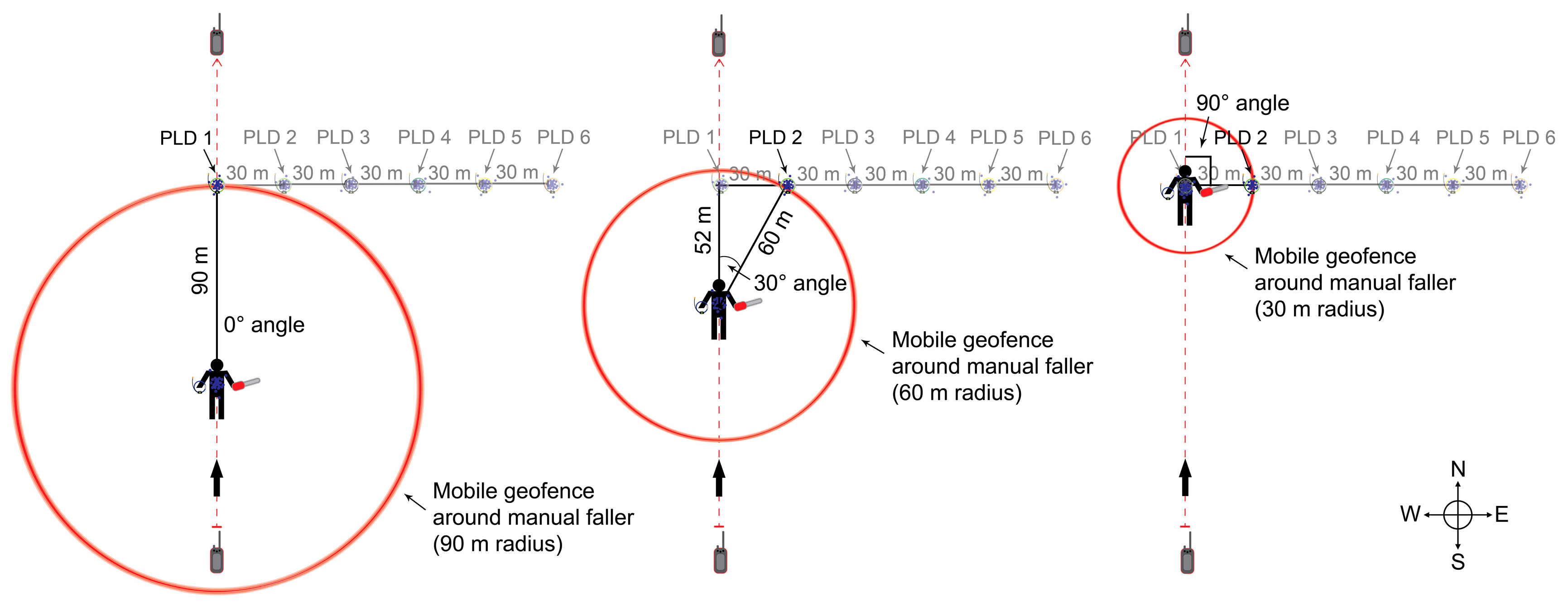
| PLD | Radius (m) | Angle (Degrees) |
|---|---|---|
| 1 | 30 | 0 |
| 2 | 30 | 90 |
| 1 | 45 | 0 |
| 2 | 45 | 42 |
| 1 | 60 | 0 |
| 2 | 60 | 30 |
| 3 | 60 | 90 |
| 1 | 75 | 0 |
| 2 | 75 | 24 |
| 3 | 75 | 53 |
| 1 | 90 | 0 |
| 2 | 90 | 19 |
| 3 | 90 | 42 |
| 4 | 90 | 90 |
| 1 | 105 | 0 |
| 2 | 105 | 17 |
| 3 | 105 | 35 |
| 4 | 105 | 59 |
| 1 | 120 | 0 |
| 2 | 120 | 14 |
| 3 | 120 | 30 |
| 4 | 120 | 49 |
| 5 | 120 | 90 |
| Model | DF 1 | AIC 2 | BIC 3 | Log Lik 4 | Test | L Ratio 5 | p-Value 6 |
|---|---|---|---|---|---|---|---|
| 1 | 210 | 4394.911 | 5325.49 | −1987.456 | - | - | - |
| 2 | 211 | 4162.837 | 5097.848 | −1870.418 | 1 vs. 2 | 234.074 | <0.0001 |
| Model Term | Num DF 1 | Den DF 2 | F-Statistic 3 | p-Value 4 |
|---|---|---|---|---|
| (Intercept) | 1 | 396 | 8.43367 | 0.0039 |
| Rad Ang | 22 | 396 | 76.00023 | <0.0001 |
| Pace | 2 | 16 | 1.24997 | 0.313 |
| TI | 2 | 16 | 1.16111 | 0.3382 |
| RadAng: Pace | 44 | 396 | 0.937 | 0.5896 |
| RadAng: TI | 44 | 396 | 0.83993 | 0.7571 |
| Pace: TI | 4 | 16 | 0.60202 | 0.6667 |
| RadAng:Pace: TI | 88 | 396 | 1.24072 | 0.0874 |
| Parameter | Estimate 1 | Std. Error 2 | t-Statistic 3 | p-Value 4 |
|---|---|---|---|---|
| b0 | 3.86 × 100 | 1.35 × 10⁻² | 286.41 | <2 × 10⁻¹⁶ |
| b1 | −5.79 × 10⁻² | 3.64 × 10⁻⁴ | −159.06 | <2 × 10⁻¹⁶ |
| b2 | 6.92 × 10⁻² | 7.33 × 10⁻⁵ | 944.50 | <2 × 10⁻¹⁶ |
| b3 | −2.00 × 100 | 2.03 × 10⁻³ | −985.52 | <2 × 10⁻¹⁶ |
| b4 | −4.29 × 10⁻³ | 1.27 × 10⁻⁴ | −33.76 | <2 × 10⁻¹⁶ |
© 2017 by the authors. Licensee MDPI, Basel, Switzerland. This article is an open access article distributed under the terms and conditions of the Creative Commons Attribution (CC BY) license (http://creativecommons.org/licenses/by/4.0/).
Share and Cite
Zimbelman, E.G.; Keefe, R.F.; Strand, E.K.; Kolden, C.A.; Wempe, A.M. Hazards in Motion: Development of Mobile Geofences for Use in Logging Safety. Sensors 2017, 17, 822. https://doi.org/10.3390/s17040822
Zimbelman EG, Keefe RF, Strand EK, Kolden CA, Wempe AM. Hazards in Motion: Development of Mobile Geofences for Use in Logging Safety. Sensors. 2017; 17(4):822. https://doi.org/10.3390/s17040822
Chicago/Turabian StyleZimbelman, Eloise G., Robert F. Keefe, Eva K. Strand, Crystal A. Kolden, and Ann M. Wempe. 2017. "Hazards in Motion: Development of Mobile Geofences for Use in Logging Safety" Sensors 17, no. 4: 822. https://doi.org/10.3390/s17040822
APA StyleZimbelman, E. G., Keefe, R. F., Strand, E. K., Kolden, C. A., & Wempe, A. M. (2017). Hazards in Motion: Development of Mobile Geofences for Use in Logging Safety. Sensors, 17(4), 822. https://doi.org/10.3390/s17040822