
An Improved Multi-Sensor Fusion Navigation Algorithm Based on the Factor Graph


Abstract
:1. Introduction
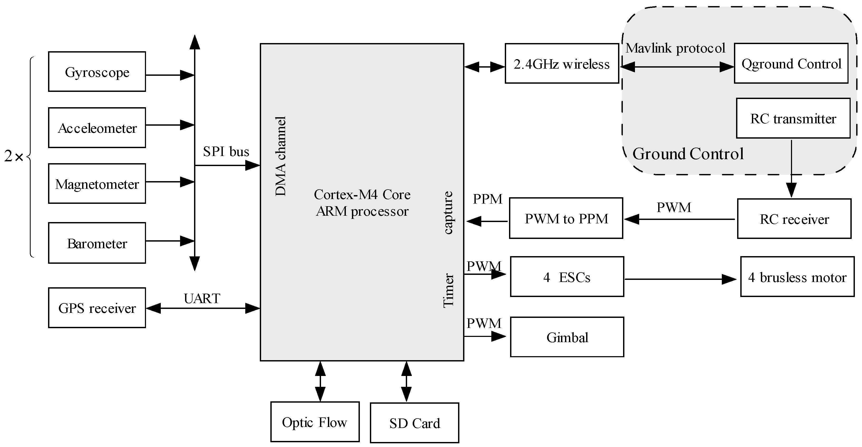
2. System Overview
- MPU-6000 inertial sensor, including a three-axis MEMS gyroscope and a three-axis accelerometer.
- HMC5983 magnetometer enables 1° to 2° compass heading accuracy with temperature compensation.
- MS5611 barometer module, with an altitude resolution of 0.1 m.
- URM37 sonar module provides 0.04 m–5 m non-contact measurement function, the ranging accuracy can reach to 1 cm.
- Ublox LEA 6H GPS receiver, with the position accuracy of 2 m.
- Optical flow sensor processing the pixel resolution of 752 × 480 at 120 (indoor) to 250 Hz (outdoor).
3. System Model for the Navigation System
3.1. State Model of the System
3.2. Measurement Model of the System
3.2.1. GPS Measurement Equation
3.2.2. Barometric Altimeter Measurement Equation
3.2.3. Magnetometer Measurement Equation
3.2.4. Optical Flow Measurement Equation
3.2.5. Sonar Measurement Equation
4. Information Fusion Method Based on the Factor Graph
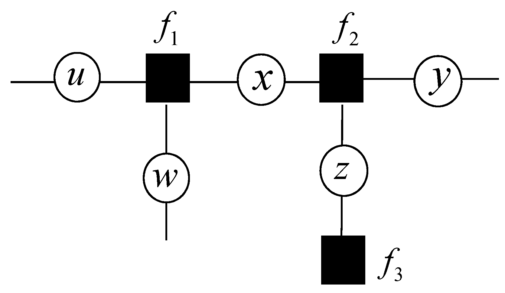
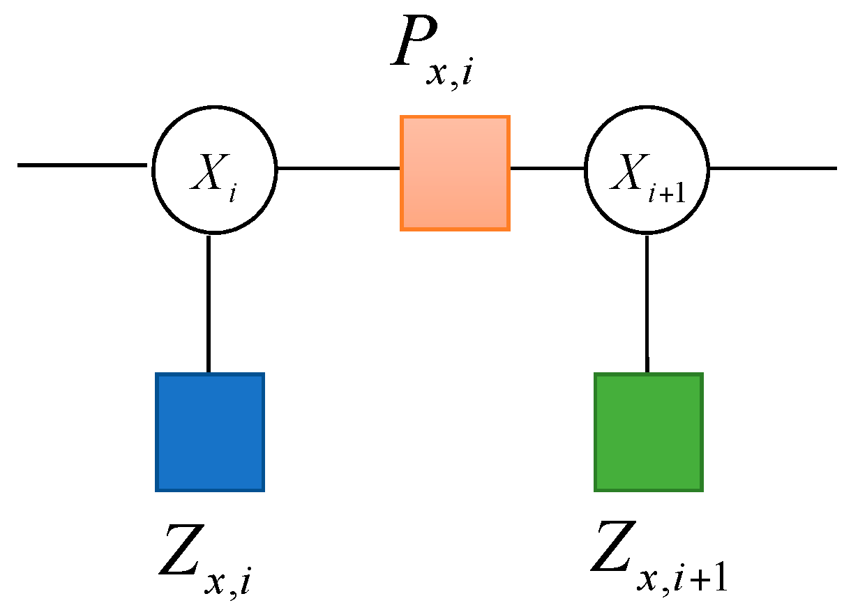
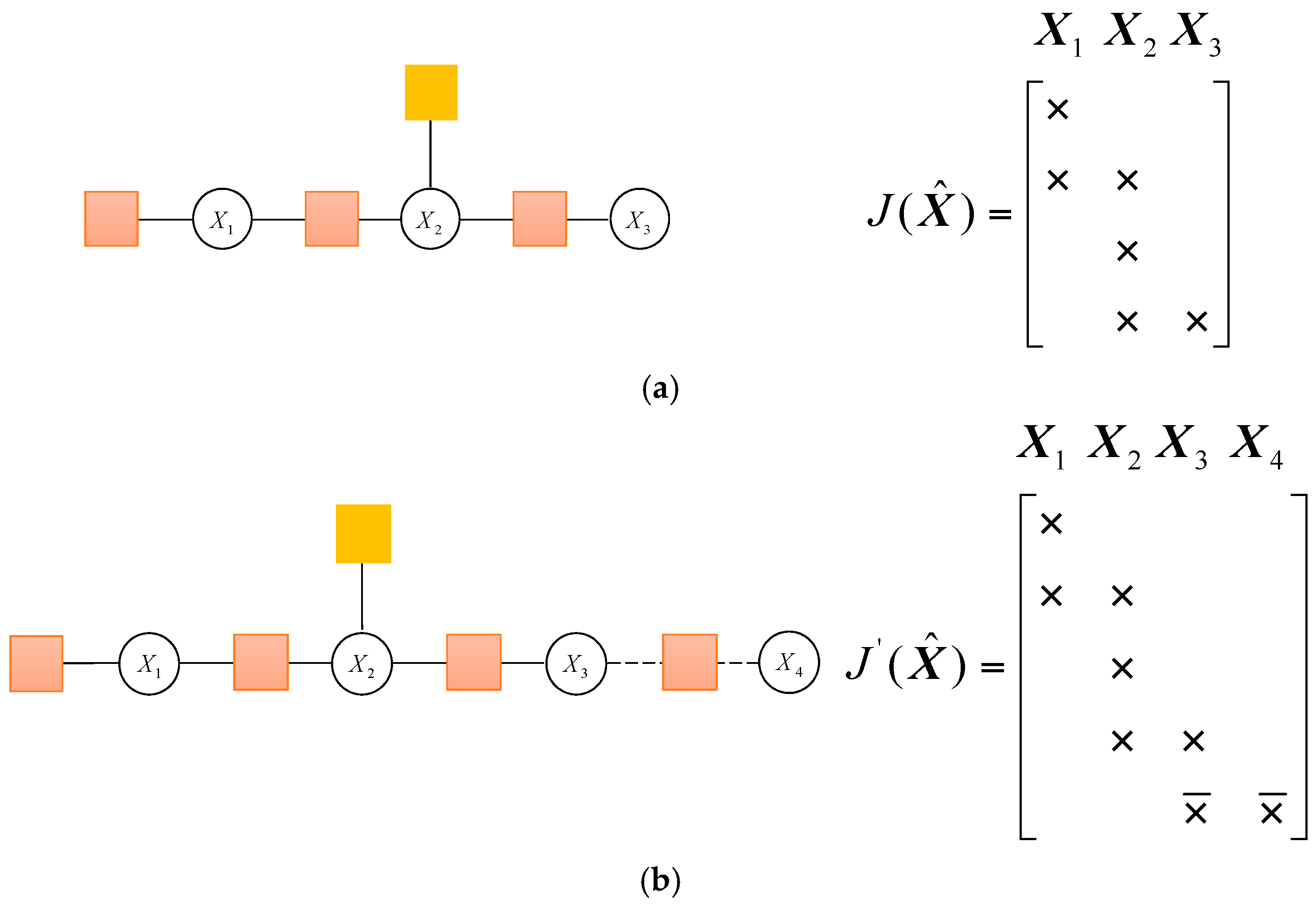
4.1. Factor Graph Formulations
4.2. Fusion Algorithm with the Factor Graph
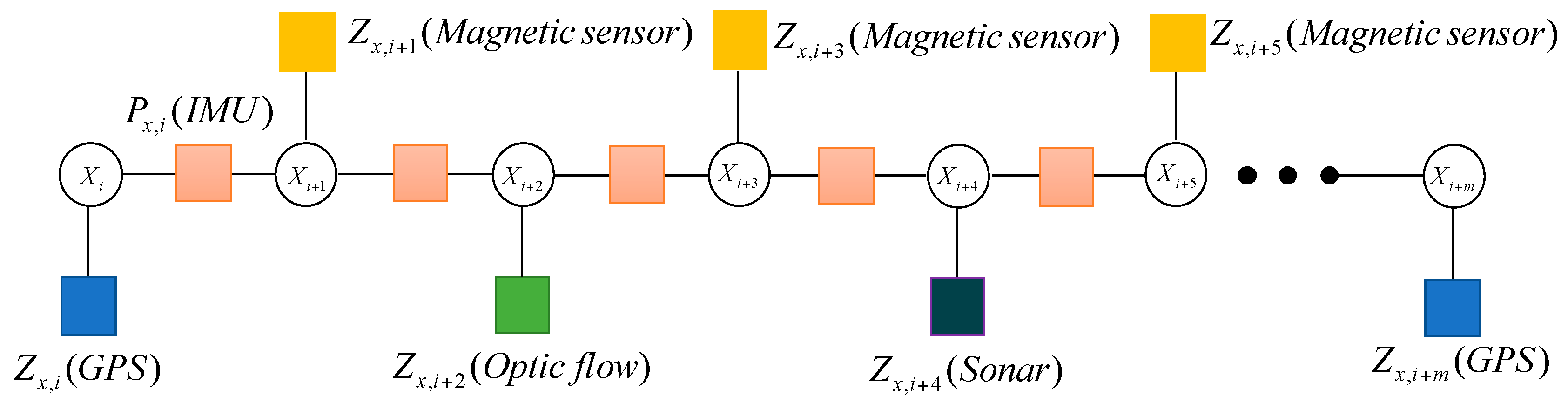
4.3. Factor Graph Modeling
- Step 1:
- Set the initial parameters and define a state-space vector. New factors and new variables are initialized. The probability density function should be set up according to the parameters of the system.
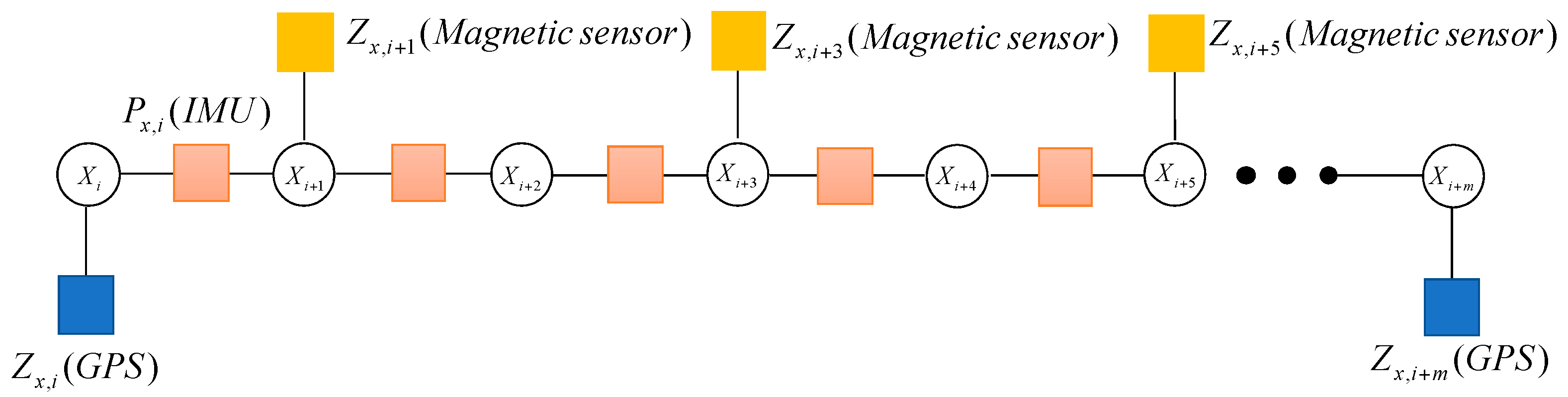
- Step 2:
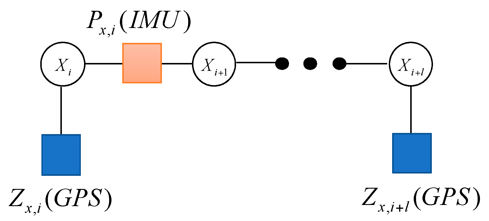
- When the system receives the IMU measurement , at moment, the factor node will be added into the graph. It connects two different variable nodes and in and moments, respectively. The IMU measurement is used to calculate the state transition matrix to predict by state vector propagation.
- Position is calculated by ;
- Velocity is calculated by ;
- Attitude is calculated by .
- Step 3:
- Add to ;
- Step 4:
- When the system receives the measurement (magnetic, GPS, sonar or optic flow, etc.) at moment, the factor node (magnetic, GPS, sonar or optic flow, etc.) will be added into the graph. Add to .
- Step 5:
- The optimization problem encoded by the factor graph is solved by Gauss–Newton iterations. is the set of all measurements, and represents the set of all variables. is an initial estimate of . According to Equation (17), the increment needs to be calculated, which should satisfy Equation (23).where is the Jacobian matrix and is the residual of all measurements.
5. Experiment and Discussion
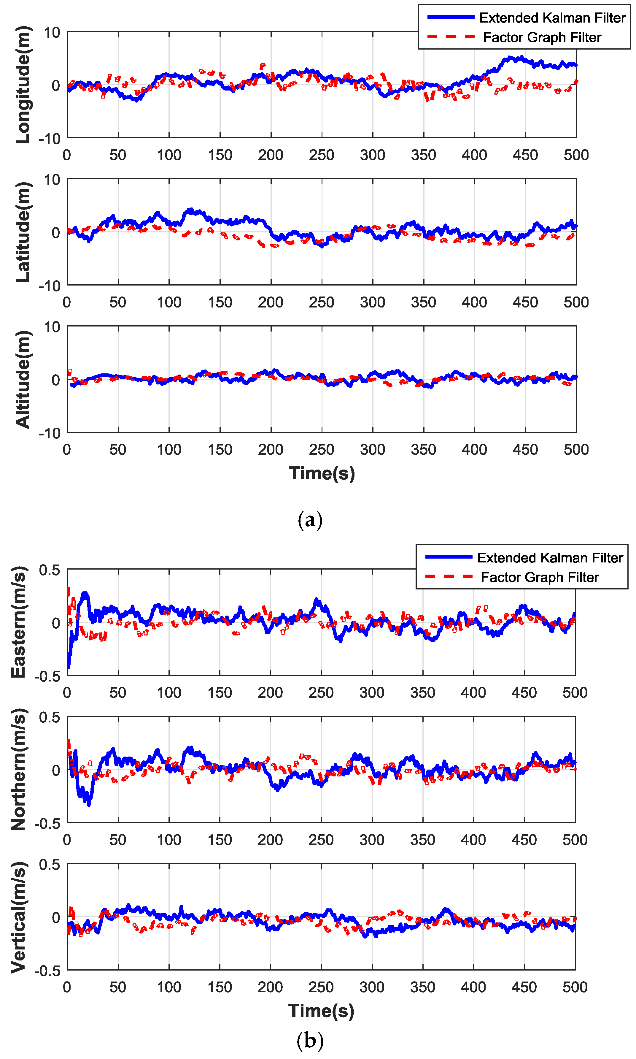
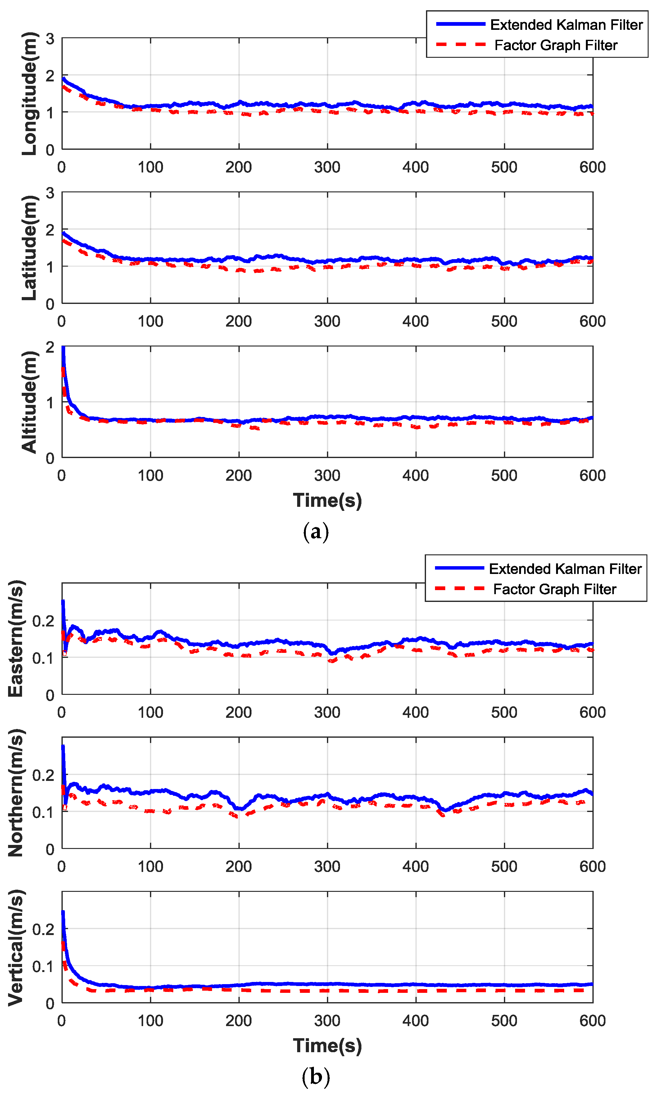
5.1. Simulation and Analysis
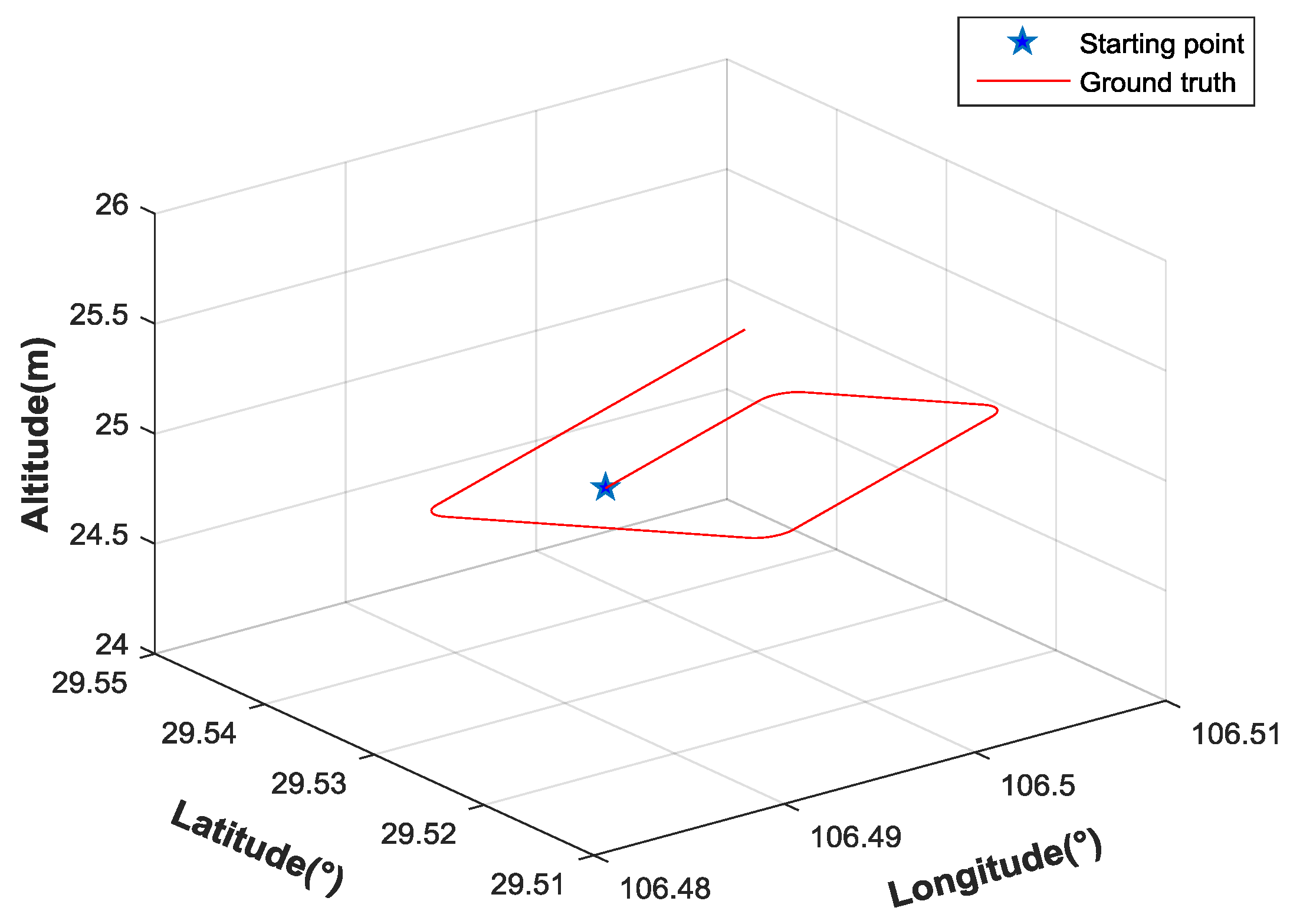
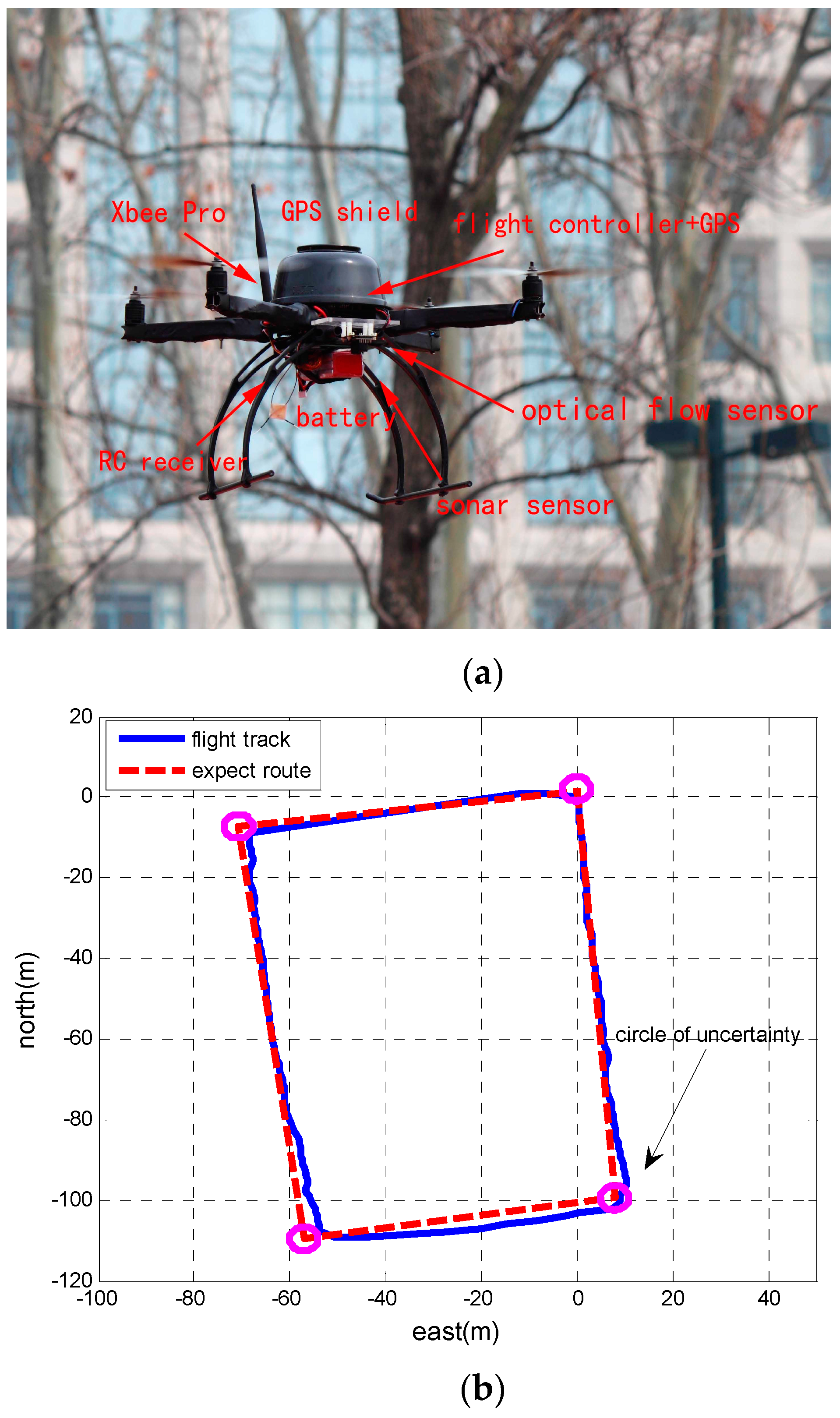
5.2. MUAV Flight Test and Results
6. Conclusions
Acknowledgments
Author Contributions
Conflicts of Interest
References
- Gökçe, F.; Üçoluk, G.; Şahin, E.; Kalkan, S. Vision-Based Detection and Distance Estimation of Micro Unmanned Aerial Vehicles. Sensors 2015, 15, 23805–23846. [Google Scholar] [CrossRef] [PubMed]
- Kim, J.H.; Sukkarieh, S. A baro-altimeter augmented INS/GPS navigation system for an uninhabited aerial vehicle. In Proceedings of the 6th International Conference on Satellite Navigation Technology (SATNAV 03), Melbourne VIC, Australia, 23–25 July 2003.
- Siebert, S.; Teizer, J. Mobile 3D mapping for surveying earthwork projects using an Unmanned Aerial Vehicle (UAV) system. Autom. Constr. 2014, 41, 1–14. [Google Scholar] [CrossRef]
- Baiocchi, V.; Dominici, D.; Milone, M.V.; Mormile, M. Development of a software to plan UAVs stereoscopic flight: An application on post earthquake scenario in L’Aquila city. In Proceedings of the International Conference on Computational Science and Its Applications, Ho Chi Minh City, Vietnam, 24–27 June 2013; Springer: Berlin/Heidelberg, Germany, 2013; pp. 150–165. [Google Scholar]
- D’Oleire-Oltmanns, S.; Marzolff, I.; Peter, K.D.; Ries, J.B. Unmanned aerial vehicle (UAV) for monitoring soil erosion in Morocco. Remote Sens. 2012, 4, 3390–3416. [Google Scholar] [CrossRef]
- Wendel, J.; Meister, O.; Schlaile, C.; Trommer, G.F. An integrated GPS/MEMS-IMU navigation system for an autonomous helicopter. Aerosp. Sci. Technol. 2006, 10, 527–533. [Google Scholar] [CrossRef]
- Chiabrando, F.; Nex, F.; Piatti, D.; Rinaudo, F. UAV and RPV systems for photogrammetric surveys in archaelogical areas: Two tests in the Piedmont region (Italy). J. Archaeol. Sci. 2011, 38, 697–710. [Google Scholar] [CrossRef]
- Li, Y. Optimal multisensor integrated navigation through information space approach. Phys. Commun. 2014, 13, 44–53. [Google Scholar] [CrossRef]
- Noureldin, A.; Osman, A.; El-Sheimy, N. A neuro-wavelet method for multi-sensor system integration for vehicular navigation. Meas. Sci. Technol. 2003, 15, 404. [Google Scholar] [CrossRef]
- Gao, S.; Zhong, Y.; Zhang, X.; Shirinzadeh, B. Multi-sensor optimal data fusion for INS/GPS/SAR integrated navigation system. Aerosp. Sci. Technol. 2009, 13, 232–237. [Google Scholar] [CrossRef]
- Grewal, M.S.; Weill, L.R.; Andrews, A.P. Global Positioning Systems, Inertial Navigation, and Integration; John Wiley & Sons: Hoboken, NJ, USA, 2007. [Google Scholar]
- Smith, D.; Singh, S. Approaches to multisensor data fusion in target tracking: A survey. IEEE Trans. Knowl. Data Eng. 2006, 18, 1696–1710. [Google Scholar] [CrossRef]
- Yager, R.R. On the fusion of imprecise uncertainty measures using belief structures. Inf. Sci. 2011, 181, 3199–3209. [Google Scholar] [CrossRef]
- Sun, X.J.; Gao, Y.; Deng, Z.L.; Wang, J.W. Multi-model information fusion Kalman filtering and white noise deconvolution. Inf. Fusion 2010, 11, 163–173. [Google Scholar] [CrossRef]
- Willner, D.; Chang, C.B.; Dunn, K.P. Kalman filter algorithms for a multi-sensor system. In Proceedings of the 1976 IEEE Conference on 15th Symposium on Adaptive Processes, Clearwater, FL, USA, 1–3 December 1976; pp. 570–574.
- Sun, S.L.; Deng, Z.L. Multi-sensor optimal information fusion Kalman filter. Automatica 2004, 40, 1017–1023. [Google Scholar] [CrossRef]
- Rodríguez-Valenzuela, S.; Holgado-Terriza, J.A.; Gutiérrez-Guerrero, J.M.; Muros-Cobos, J.L. Distributed Service-Based Approach for Sensor Data Fusion in IoT Environments. Sensors 2014, 14, 19200–19228. [Google Scholar] [CrossRef] [PubMed]
- Deng, Z.L.; Qi, R.B. Multi-sensor information fusion suboptimal steady-state Kalman filter. Chin. Sci. Abstr. 2000, 6, 183–184. [Google Scholar]
- Gan, Q.; Harris, C.J. Comparison of two measurement fusion methods for Kalman-filter-based multisensor data fusion. IEEE Trans. Aerosp. Electron. Syst. 2001, 37, 273–279. [Google Scholar] [CrossRef]
- Ali, J.; Fang, J.C. SINS/ANS/GPS integration using federated Kalman filter based on optimized information-sharing coefficients. In Proceedings of the AIAA Guidance, Navigation, and Control Conference, San Francisco, CA, USA, 15–18 August 2005; pp. 1–13.
- Brion, V.; Riff, O.; Descoleaux, M.; Mangiri, J.F.; Le Bihan, D.; Poupon, C.; Poupon, F. The Parallel Kalman Filter: An efficient tool to deal with real-time non central χ noise correction of HARDI data. In Proceedings of the IEEE International Symposium on Biomedical Imaging, Barcelona, Spain, 2–5 May 2012; pp. 34–37.
- Leung, Y.; Ji, N.N.; Ma, J.H. An integrated information fusion approach based on the theory of evidence and group decision-making. Inf. Fusion 2013, 14, 410–422. [Google Scholar] [CrossRef]
- Wen, C.; Wen, C.; Li, Y. An Optimal Sequential Decentralized Filter of Discrete-time Systems with Cross-Correlated Noises. In Proceedings of the 17th World Congress on the International Federation of Automatic Control, Seoul, Korea, 6–11 July 2008; pp. 7560–7565.
- Wen, C.; Cai, Y.; Wen, C.; Xu, X. Optimal sequential Kalman filtering with cross-correlated measurement noises. Aerosp. Sci. Technol. 2013, 26, 153–159. [Google Scholar] [CrossRef]
- Indelman, V.; Williams, S.; Kaess, M.; Dellaert, F. Information fusion in navigation systems via factor graph based incremental smoothing. Robot. Auton. Syst. 2013, 61, 721–738. [Google Scholar] [CrossRef]
- Loeliger, H.A.; Dauwels, J.; Hu, J.; Korl, S.; Ping, L.; Kschischang, F.R. The factor graph approach to model-based signal processing. Proc. IEEE 2007, 95, 1295–1322. [Google Scholar] [CrossRef]
- Mao, Y.; Kschischang, F.R.; Li, B.; Pasupathy, S. A factor graph approach to link loss monitoring in wireless sensor networks. IEEE J. Sel. Areas Commun. 2005, 23, 820–829. [Google Scholar]
- Forster, C.; Carlone, L.; Dellaert, F.; Scaramuzza, D. IMU Preintegration on Manifold for Efficient Visual-Inertial Maximum-a-Posteriori Estimation. Robotics: Science and Systems XI. 2015 (EPFL-CONF-214687). Available online: http://www.roboticsproceedings.org/rss11/p06.pdf (accessed on 20 March 2017).


| Sensor | Error | Value | Frequency |
|---|---|---|---|
| IMU | Gyro constant drift | 10°/h | 50 Hz |
| Gyro first-order Markov process | 10°/h | ||
| Gyro white noise measurement | 10°/h | ||
| Accelerometer first-order Markov process | 1 × 10⁻⁴ g | ||
| GPS | Position error noise | 10 m, 10 m, 20 m | 1 Hz |
| Velocity error noise | 0.1 m/s, 0.1 m/s, 0.1 m/s | ||
| Magnetometer | Heading error noise | 0.2° | 20 Hz |
| Barometer | Height error noise | 5 m | 10 Hz |
| Error Type | Average RMSE in the Position Error (units: m) | Average RMSE in the Velocity Error (units: m/s) | ||||
|---|---|---|---|---|---|---|
| Longitude | Latitude | Height | Eastern | Northern | Vertical | |
| Extend Kalman filter | 1.212 | 1.205 | 0.703 | 0.141 | 0.142 | 0.049 |
| Factor graph filter | 1.043 | 1.035 | 0.628 | 0.121 | 0.115 | 0.034 |
| Type | Parameters Item | Unit |
|---|---|---|
| Machine size | 608 × 608 × 243 | mm |
| Takeoff weight | 950 | g |
| Maximum payload | <580 | g |
| Flight time | 15 | min |
| Error Type | RMSE in the Position Error (units: m) | RMSE in the Velocity Error (units: m/s) | ||||
|---|---|---|---|---|---|---|
| Longitude | Latitude | Height | Eastern | Northern | Vertical | |
| Extend Kalman filter | 1.821 | 1.451 | 0.652 | 0.088 | 0.086 | 0.061 |
| Factor graph filter | 1.288 | 1.143 | 0.519 | 0.065 | 0.061 | 0.049 |
© 2017 by the authors. Licensee MDPI, Basel, Switzerland. This article is an open access article distributed under the terms and conditions of the Creative Commons Attribution (CC BY) license ( http://creativecommons.org/licenses/by/4.0/).
Share and Cite
Zeng, Q.; Chen, W.; Liu, J.; Wang, H. An Improved Multi-Sensor Fusion Navigation Algorithm Based on the Factor Graph. Sensors 2017, 17, 641. https://doi.org/10.3390/s17030641
Zeng Q, Chen W, Liu J, Wang H. An Improved Multi-Sensor Fusion Navigation Algorithm Based on the Factor Graph. Sensors. 2017; 17(3):641. https://doi.org/10.3390/s17030641
Chicago/Turabian StyleZeng, Qinghua, Weina Chen, Jianye Liu, and Huizhe Wang. 2017. "An Improved Multi-Sensor Fusion Navigation Algorithm Based on the Factor Graph" Sensors 17, no. 3: 641. https://doi.org/10.3390/s17030641
APA StyleZeng, Q., Chen, W., Liu, J., & Wang, H. (2017). An Improved Multi-Sensor Fusion Navigation Algorithm Based on the Factor Graph. Sensors, 17(3), 641. https://doi.org/10.3390/s17030641