
Parameter Selection and Performance Comparison of Particle Swarm Optimization in Sensor Networks Localization


Abstract
:1. Introduction
- Ease of implementation on hardware or software.
- High-quality solutions because of its ability to escape from local optima.
- Quick convergence.
- It surveys the popular particle swarm optimization variants and particle swarm optimization-based localization algorithms for wireless sensor networks.
- It presents parameter selection of nine particle swarm optimization variants and six types of swarm topologies by extensive simulations.
- It comprehensively compares the performance of these algorithms.
2. Statements of Localization Problem and PSO
2.1. Localization Problem for Static WSNs
2.2. Particle Swarm Optimization
- Ring topology: Each particle is affected by its k immediate neighbors.
- Star/Wheel topology: Only one particle is in the center of the swarm, and this particle is influenced by all other particles. However, each of the other particles can only access the information of the central particle.
- Pyramid topology: The swarm of particles are divided into several levels, and there are particles in level l (), which form a mesh.
- Von Neumann topology: All particles are connected as a toroidal, and each particle has four neighbors, which are above, below, left, and right particles.
- Random topology: Each particle chooses neighbors randomly at each iteration. We utilize the second algorithm proposed in [24] to generate the random topology.
2.3. Evaluation Criteria of PSO-Based Localization Algorithms
- Localization error. The localization error of unknown node is defined as . The mean and standard deviation of localization error are denoted by and , respectively.
- Number of iterations. This is the number of iterations of PSO to achieve the best fitness. The mean and standard deviation of the number of iterations are denoted by and , respectively.
3. A Survey of PSO-Based Localization Algorithms
3.1. Basic Procedure of PSO-Based Localization Algorithms
| Algorithm 1 PSO-Based Localization Algorithm |
|
3.2. PSO-Based Localization Algorithms
- H-Best PSO (HPSO). Global- and local-best PSO algorithms have their own advantages and disadvantages. Combining these two algorithms, HPSO [9,14] divides the particles into several groups, and particle i is updated based on , , and , per the following equation:Here, is the same as of (10), and is a random number uniformly distributed in . HPSO provides fast convergence and swarm diversity, but it utilizes more parameters than WPSO.
- PSO with particle permutation (PPSO). In order to speed up the convergence, PPSO [37] sorts all particles such that , if , and replaces the positions of particles to M with positions close to . The rule of replacement is:where is a random number uniformly distributed in (−0.5,0.5).
- Extremum disturbed and simple PSO (EPSO). Sometimes, PSO easily fall into local extrema. EPSO [38] uses two preset thresholds and to randomly churn and to overcome this shortcoming. The operators of extremal perturbation are:Let and be evolutionary stagnation iterations of and , respectively. In (14), if (), () is 1; Otherwise, () is a random number uniformly distributed in [0,1]. For particle i, the update function of EPSO iswhere is used to control the movement direction of particle i to make the algorithm convergence fast, which is defined as
- Dynamic PSO (DPSO). Each particle in DPSO [19] pays full attention to the historical information of all neighboring particles, instead of only focusing on the particle which gets the optimum position in the neighborhood. For particle i, the update function of DPSO iswhere K is the number of neighboring particles of the ith particle. is the previous position of the ith particle. Note that , , and are just weights without physical meaning.
- Binary PSO (BPSO). BPSO [39] is used in binary discrete search space, which applies a sigmoid transformation to the speed attribute in update function, so its update function of particle i iswhere is defined asis a random number.
- PSO with particle migration (MPSO) [40]. MPSO enhances the diversity of particles and avoids premature convergence. MPSO randomly partitions particles into several sub-swarms, each of which evolves based on TPSO, and some particles migrate from one sub-swarm to another during evolution.
3.3. Comparison between PSO and Other Optimization Algorithms
4. Parameter Selections of PSO-Based Localization Algorithms
4.1. Simulation Setup
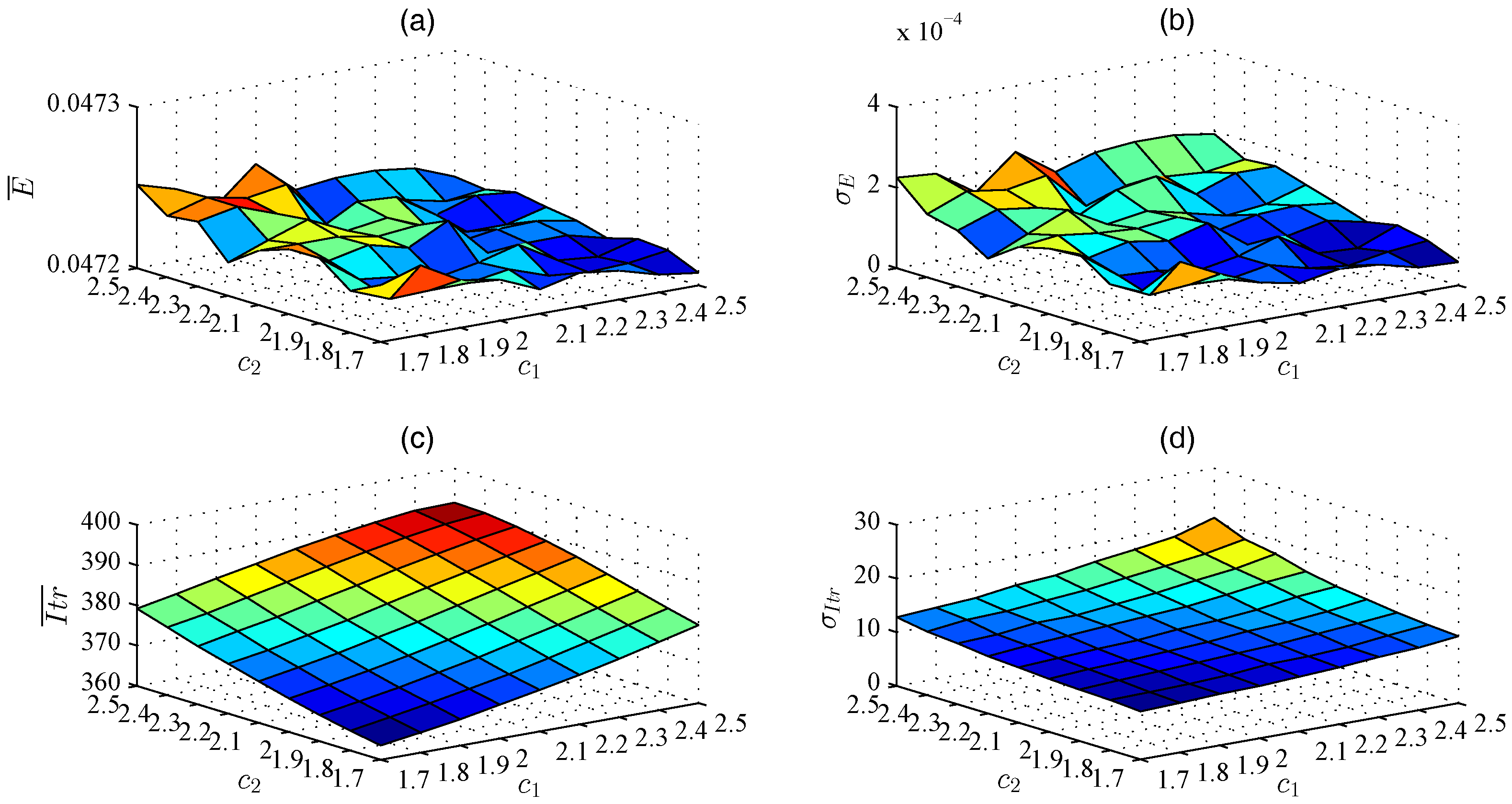
- Using and to find out the best , , , and ω.
- Using the best , , and ω to choose M.
- Using the best , , , ω and M to choose .
- Using the best , , , ω, M and to compare fitness functions.
4.2. Best Parameters of PSO-Based Localization Algorithms
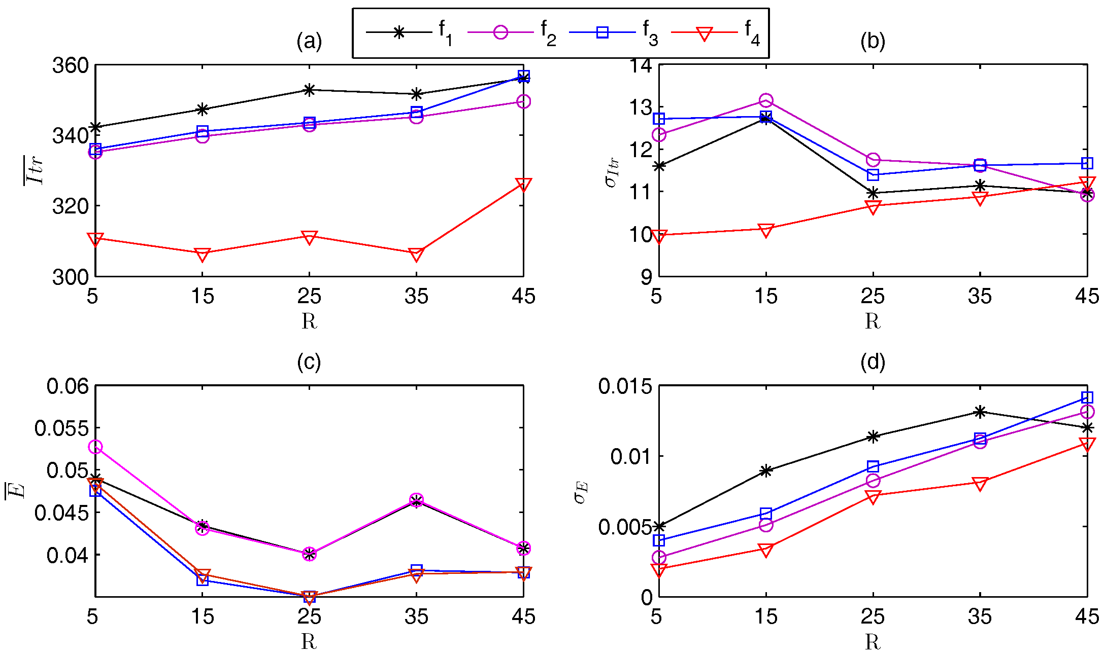
4.3. Performance Comparison of Fitness Function
5. Performance Comparisons of PSO-Based Localization Algorithms
5.1. Simulations Setup
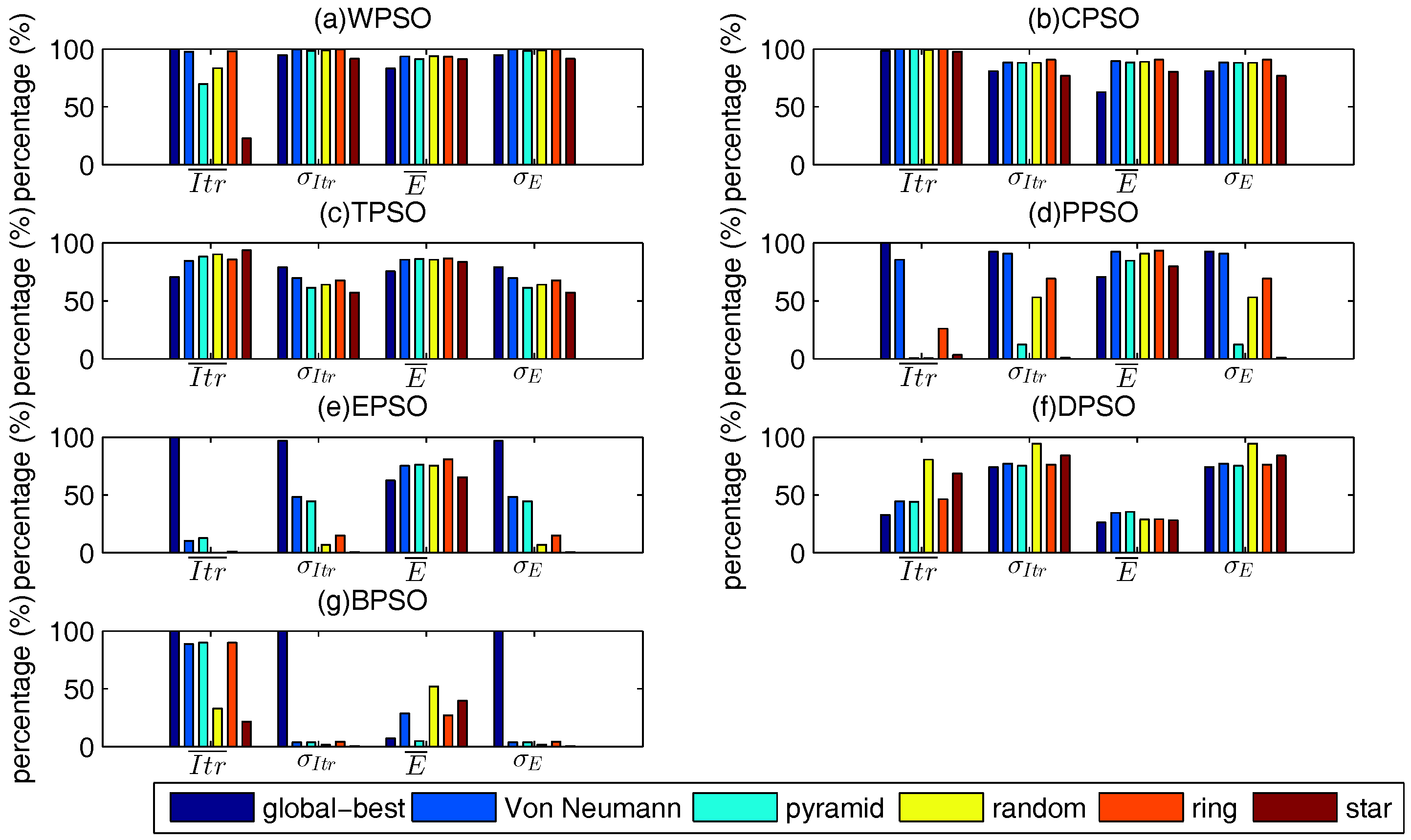
5.2. Comparisons of Different Swarm Topologies in Same PSO
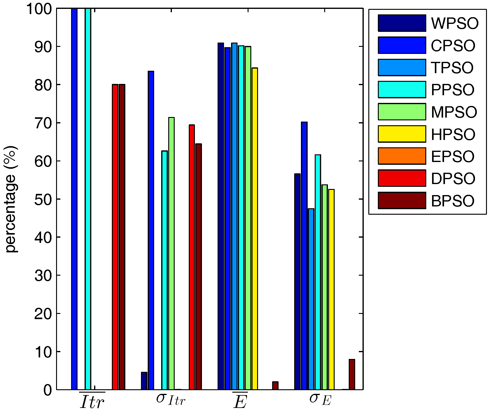
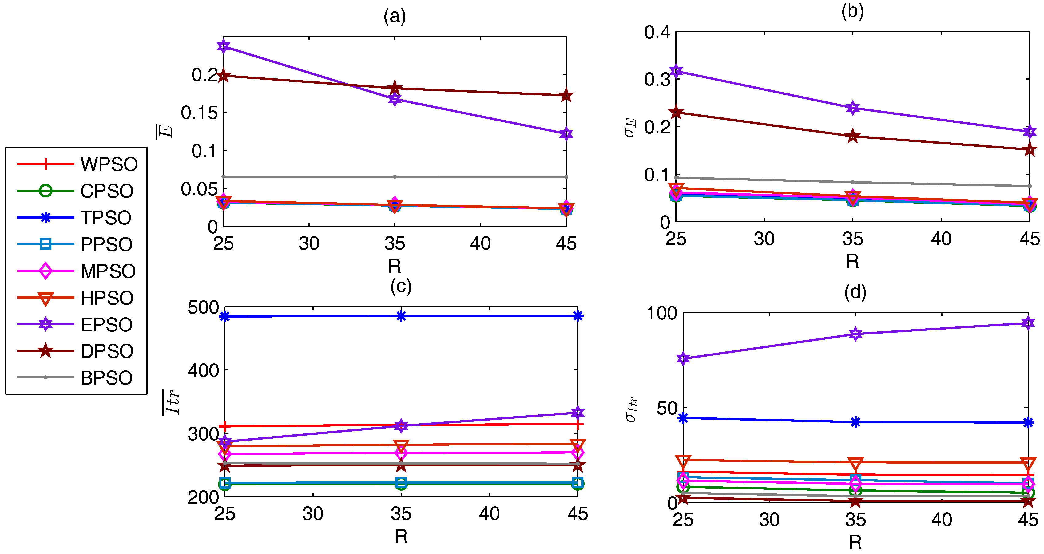
5.3. Comparison of PSO-Based Localization Algorithms
5.3.1. General Analysis
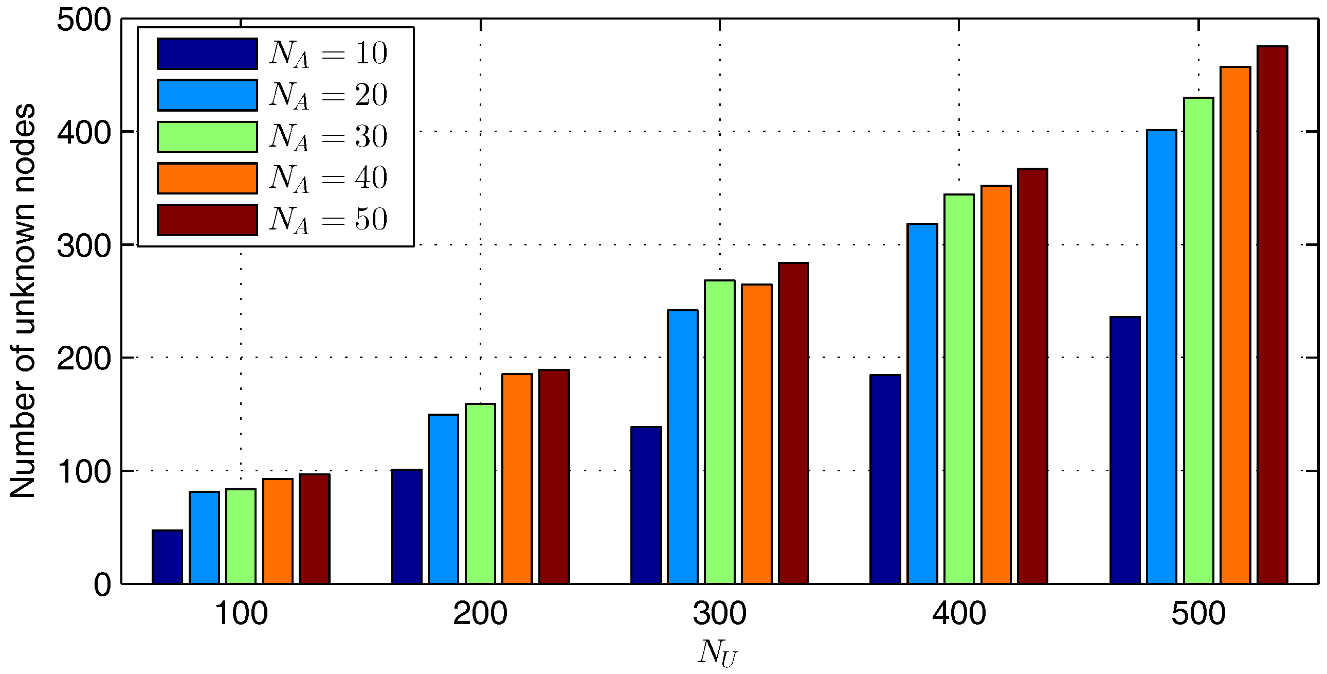
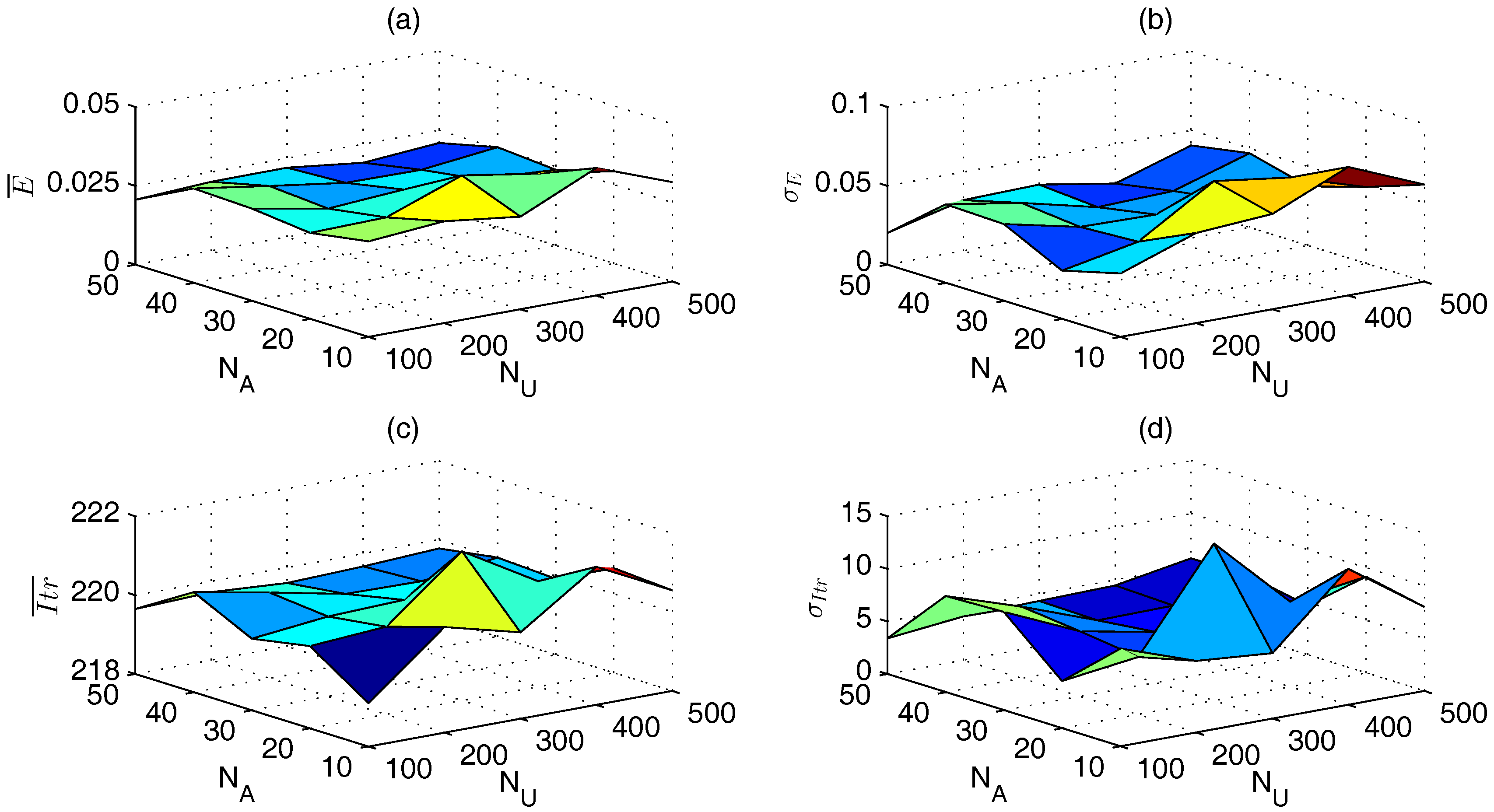
5.3.2. Impacts of Network Parameters on Performance
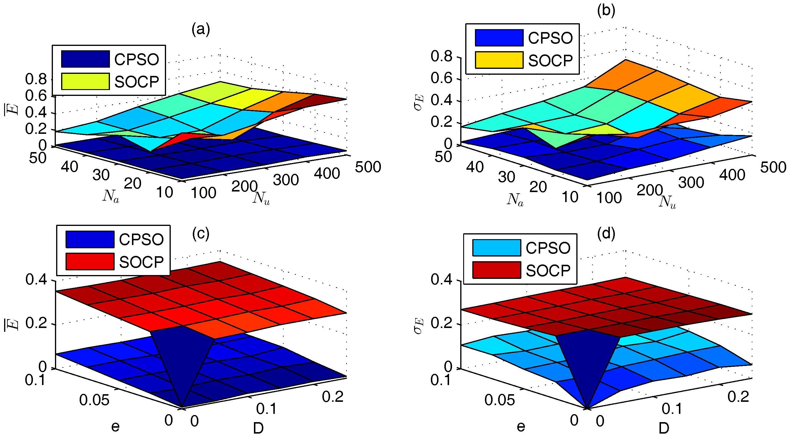
5.4. Comparison between CPSO and SOCP
6. Conclusions
Acknowledgments
Author Contributions
Conflicts of Interest
References
- Yick, J.; Mukherjee, B.; Ghosal, D. Wireless sensor network survey. Comput. Netw. 2008, 52, 2292–2330. [Google Scholar] [CrossRef]
- Cheng, L.; Wu, C.; Zhang, Y.; Wu, H.; Li, M.; Maple, C. A survey of localization in wireless sensor network. Int. J. Distrib. Sens. Netw. 2012, 2012, 962523. [Google Scholar] [CrossRef]
- Han, G.; Xu, H.; Duong, T.Q.; Jiang, J.; Hara, T. Localization algorithms of wireless sensor networks: A survey. Telecommun. Syst. 2011, 48, 1–18. [Google Scholar]
- Naddafzadeh-Shirazi, G.; Shenouda, M.B.; Lampe, L. Second order cone programming for sensor network localization with anchor position uncertainty. IEEE Trans. Wirel. Commun. 2014, 13, 749–763. [Google Scholar] [CrossRef]
- Beko, M. Energy-based localization in wireless sensor networks using second-order cone programming relaxation. Wirel. Pers. Commun. 2014, 77, 1847–1857. [Google Scholar] [CrossRef]
- Erseghe, T. A distributed and maximum-likelihood sensor network localization algorithm based upon a nonconvex problem formulation. IEEE Trans. Signal Inf. Process. Netw. 2015, 1, 247–258. [Google Scholar] [CrossRef]
- Ghari, P.M.; Shahbazian, R.; Ghorashi, S.A. Wireless sensor network localization in harsh environments using SDP relaxation. IEEE Commun. Lett. 2016, 20, 137–140. [Google Scholar] [CrossRef]
- Kulkarni, R.V.; Förster, A.; Venayagamoorthy, G.K. Computational intelligence in wireless sensor networks: A survey. IEEE Commun. Surv. Tutor. 2011, 13, 68–96. [Google Scholar] [CrossRef]
- Kumar, A.; Khoslay, A.; Sainiz, J.S.; Singh, S. Computational intelligence based algorithm for node localization in wireless sensor networks. In Proceedings of the 2012 6th IEEE International Conference Intelligent Systems (IS), Sofia, Bulgaria, 6–8 September 2012; pp. 431–438.
- Cheng, J.; Xia, L. An effective Cuckoo search algorithm for node localization in wireless sensor network. Sensors 2016, 16, 1390. [Google Scholar] [CrossRef] [PubMed]
- Chuang, P.J.; Jiang, Y.J. Effective neural network-based node localisation scheme for wireless sensor networks. IET Wirel. Sens. Syst. 2014, 4, 97–103. [Google Scholar] [CrossRef]
- Kulkarni, R.V.; Venayagamoorthy, G.K.; Cheng, M.X. Bio-inspired node localization in wireless sensor networks. In Proceedings of the IEEE International Conference on Systems, Man and Cybernetics (SMC 2009), San Antonio, TX, USA, 11–14 October 2009; pp. 205–210.
- Goyal, S.; Patterh, M.S. Modified bat algorithm for localization of wireless sensor network. Wirel. Pers. Commun. 2016, 86, 657–670. [Google Scholar] [CrossRef]
- Kumar, A.; Khoslay, A.; Sainiz, J.S.; Singh, S. Meta-heuristic range based node localization algorithm for wireless sensor networks. In Proceedings of the 2012 International Conference on Localization and GNSS (ICL-GNSS), Starnberg, Germany, 25–27 June 2012; pp. 1–7.
- Li, Z.; Liu, X.; Duan, X. Comparative research on particle swarm optimization and genetic algorithm. Comput. Inf. Sci. 2010, 3, 120–127. [Google Scholar]
- Jordehi, A.R.; Jasni, J. Parameter selection in particle swarm optimization: A survey. J. Exp. Theor. Artif. Intell. 2013, 25, 527–542. [Google Scholar] [CrossRef]
- Kulkarni, R.V.; Venayagamoorthy, G.K. Particle swarm optimization in wireless sensor networks: A brief survey. IEEE Trans. Syst. Man Cybern. C 2011, 41, 262–267. [Google Scholar] [CrossRef]
- Gharghan, S.K.; Nordin, R.; Ismail, M.; Ali, J.A. Accurate wireless sensor localization technique based on hybrid PSO-ANN algorithm for indoor and outdoor track cycling. IEEE Sens. J. 2016, 16, 529–541. [Google Scholar] [CrossRef]
- Cao, C.; Ni, Q.; Yin, C. Comparison of particle swarm optimization algorithms in wireless sensor network node localization. In Proceedings of the 2014 IEEE International Conference on Systems, Man and Cybernetics (SMC), San Diego, CA, USA, 5–8 October 2014; pp. 252–257.
- Xu, L.; Zhang, H.; Shi, W. Mobile anchor assisted node localization in sensor networks based on particle swarm optimization. In Proceedings of the 2010 6th International Conference on Wireless Communications Networking and Mobile Computing (WiCOM), Chengdu, China, 23–25 September 2010; pp. 1–5.
- Han, W.; Yang, P.; Ren, H.; Sun, J. Comparison study of several kinds of inertia weights for PSO. In Proceedings of the 2010 IEEE International Conference on Progress in Informatics and Computing (PIC), Shanghai, China, 10–12 December 2010; pp. 280–284.
- Valle, Y.D.; Venayagamoorthy, G.K.; Mohagheghi, S.; Hernandez, J.C.; Harley, R.G. Particle swarm optimization: Basic concepts, variants and applications in power systems. IEEE Trans. Evol. Comput. 2008, 12, 171–195. [Google Scholar] [CrossRef]
- Medina, A.J.R.; Pulido, G.T.; Ramírez-Torres, J.G. A comparative study of neighborhood topologies for particle swarm optimizers. In Proceeding of the International Joint Conference Computational Intelligence, Funchal, Madeira, Portugal, 5–7 October, 2009; pp. 152–159.
- Clerc, M. Back to Random Topology. Available online: http://clerc.maurice.free.fr/pso/random_topology.pdf (accessed on 28 February 2017).
- Gopakumar, A.; Jacob, L. Localization in wireless sensor networks using particle swarm optimization. In Proceeding of the IET International Conference on Wireless, Mobile and Multimedia Networks, Beijing, China, 11–12 January 2008; pp. 227–230.
- Gao, W.; Kamath, G.; Veeramachaneni, K.; Osadciw, L. A particle swarm optimization based multilateration algorithm for UWB sensor network. In Proceedings of the Canadian Conference on Electrical and Computer Engineering (CCECE ’09), Budapest, Hungary, 3–6 May 2009; pp. 950–953.
- Okamoto, E.; Horiba, M.; Nakashima, K.; Shinohara, T.; Matsumura, K. Particle swarm optimization-based low-complexity three-dimensional UWB localization scheme. In Proceedings of the 2014 Sixth International Conf on Ubiquitous and Future Networks (ICUFN), Shanghai, China, 8–11 July 2014; pp. 120–124.
- Chuang, P.J.; Wu, C.P. Employing PSO to enhance RSS range-based node localization for wireless sensor networks. J. Inf. Sci. Eng. 2011, 27, 1597–1611. [Google Scholar]
- Liu, Z.; Liu, Z. Node self-localization algorithm for wireless sensor networks based on modified particle swarm optimization. In Proceedings of the 2015 27th Chinese Control and Decision Conference (CCDC), Qingdao, China, 23–25 May 2015; pp. 5968–5971.
- Mansoor-ul-haque, F.A.K.; Iftikhar, M. Optimized energy-efficient iterative distributed localization for wireless sensor networks. In Proceedings of the 2013 IEEE International Conference on Systems, Man, and Cybernetics (SMC), Manchester, UK, 13–16 October 2013; pp. 1407–1412.
- Wei, N.; Guo, Q.; Shu, M.; Lv, J.; Yang, M. Three-dimensional localization algorithm of wireless sensor networks base on particle swarm optimization. J. China Univ. Posts Telecommun. 2012, 19, 7–12. [Google Scholar] [CrossRef]
- Dong, E.; Chai, Y.; Liu, X. A novel three-dimensional localization algorithm for wireless sensor networks based on particle swarm optimization. In Proceedings of the 2011 18th International Conference on Telecommunications (ICT), Ayia Napa, Cyprus, 8–11 May 2011; pp. 55–60.
- Zhang, Y.; Liang, J.; Jiang, S.; Chen, W. A localization method for underwater wireless sensor networks based on mobility prediction and particle swarm optimization algorithms. Sensors 2016, 16, 212. [Google Scholar] [CrossRef] [PubMed]
- Zhang, X.; Wang, T.; Fang, J. A node localization approach using particle swarm optimization in wireless sensor networks. In Proceedings of the 2014 International Conference on Identification, Information and Knowledge in the Internet of Things (IIKI), Beijing, China, 17–18 October 2014; pp. 84–87.
- Kulkarni, R.V.; Venayagamoorthy, G.K. Bio-inspired algorithms for autonomous deployment and localization of sensor nodes. IEEE Trans. Syst., Man, Cybern. C 2010, 40, 663–675. [Google Scholar] [CrossRef]
- Clerc, M.; Kennedy, J. The particle swarm-explosion, stability, and convergence in a multidimensional complex space. IEEE Trans. Evol. Comput. 2002, 6, 58–73. [Google Scholar] [CrossRef]
- Monica, S.; Ferrari, G. Swarm intelligent approaches to auto-localization of nodes in static UWB networks. Appl. Soft Comput. 2014, 25, 426–434. [Google Scholar] [CrossRef]
- Zhang, Q.; Cheng, M. A node localization algorithm for wireless sensor network based on improved particle swarm optimization. Lect. Note Elect. Eng. 2014, 237, 135–144. [Google Scholar]
- Zain, I.F.M.; Shin, S.Y. Distributed localization for wireless sensor networks using binary particle swarm optimization (BPSO). In Proceedings of the 2014 IEEE 79th Vehicular Technology Conference (VTC Spring), Seoul, Korea, 18–21 May 2014; pp. 1–5.
- Ma, G.; Zhou, W.; Chang, X. A novel particle swarm optimization algorithm based on particle migration. Appl. Math. Comput. 2012, 218, 6620–6626. [Google Scholar]
- Guo, H.; Low, K.S.; Nguyen, H.A. Optimizing the localization of a wireless sensor network in real time based on a low-cost microcontroller. IEEE Trans. Ind. Electron. 2011, 58, 741–749. [Google Scholar] [CrossRef]
- Namin, P.H.; Tinati, M.A. Node localization using particle swarm optimization. In Proceedings of the 2011 Seventh International Conference on Intelligent Sensors, Sensor Networks and Information Processing (ISSNIP), Adelaide, Australia, 6–9 December 2011; pp. 288–293.
- Liu, Q.; Wei, W.; Yuan, H.; Zha, Z.; Li, Y. Topology selection for particle swarm optimization. Inf. Sci. 2016, 363, 154–173. [Google Scholar] [CrossRef]
- Bao, H.; Zhang, B.; Li, C.; Yao, Z. Mobile anchor assisted particle swarm optimization (PSO) based localization algorithms for wireless sensor networks. Wirel. Commun. Mob. Comput. 2012, 12, 1313–1325. [Google Scholar] [CrossRef]
- CVX Research. CVX: Matlab Software for Disciplined Convex Programming. Available online: http://cvxr.com/cvx/ (accessed on 28 February 2017).


| Algorithm | References | Comparative | Advantages of PSO |
|---|---|---|---|
| WPSO | [12,35] | bacterial foraging algorithm | faster |
| WPSO | [25] | simulated annealing | more accurate |
| WPSO | [41] | Gauss–Newton algorithm | more accurate |
| WPSO | [26,31] | least square | more accurate |
| WPSO | [42] | simulated annealing, semi-definite programming | faster, more accurate |
| WPSO | [28] | artificial neural network | more accurate |
| WPSO | [32] | least square | faster, more accurate |
| HPSO | [9,14] | biogeography-based optimization | faster |
| PPSO | [37] | two-stage maximum-likelihood, plane intersection | faster, more accurate |
| Type | Values |
|---|---|
| network | R = 5:10:45, e = 0.05:0.05:0.2, = 3:20 |
| General | = 0.1R:0.1R:2R, M = 5:5:100, = 500 |
| WPSO, EPSO | = 1.4:−0.1:0.9, = 0.4:−0.1:0, = 1.7:0.1:2.5, = 1.7:0.1:2.5 |
| CPSO | = 2.05:0.05:2.5, = 2.05:0.05:2.5 |
| MPSO, TPSO | = 1.4:−0.1:0.9, = 0.4:−0.1:0, = = 3:−0.25:0.25, = = −0.25:−0.25:0.25 |
| HPSO | ω = 0.7, = = = 1.494 |
| PPSO | ω = 1, = = 2.0 |
| BPSO | ω = 1.0:−0.1:0, = 1.7:0.1:2.5, = 1.7:0.1:2.5 |
| DPSO | = 1.0:0.1:0.1, = 2.5:−0.1:1.5, = 0:0.1:1.0 |
| Variant | Topology | M | |||
|---|---|---|---|---|---|
| WPSO | global-best | [1.7–1.8,1.7–1.8,—] | [0.9,0] | 30 | |
| pyramid | [1.7,1.7–1.8,—],[1.8,1.7,—] | [0.9,0] | 21 | ||
| random | [1.7,1.7–1.8,—] | [0.9,0] | 30 | ||
| Von Neumann | [1.7,1.7–1.8,—],[1.8,1.7] | [0.9,0] | 25 | ||
| ring | [1.7,1.7–1.8,—],[1.8,1.7,—] | [0.9,0] | 25 | ||
| star | [1.7,1.7–1.8,—],[1.8,1.7,—] | [0.9,0] | 25 | ||
| CPSO | global-best | [2.4,2.5,—],[2.45,2.45–2.5,—] | — | 10 | — |
| pyramid | [2.45,2.5,—],[2.5,2.45–2.5,—] | — | 21 | — | |
| random | [2.5,2.5,—] | — | 10 | — | |
| Von Neumann | [2.45,2.45–2.5,—],[2.5,2.4–2.5,—] | — | 10 | — | |
| ring | [2.45,2.5,—],[2.5,2.4–2.5,—] | — | 10 | — | |
| star | [2.4,2.5,—],[2.45,2.45–2.5,—] | — | 10 | — | |
| TPSO | global-best | [0.5,0.25,—],[0.75–1,0.25–0.5,—] | [0.9,0] | 25 | |
| pyramid | [0.5–1,0.25,—],[0.75,0.25–0.5,—] | [0.9,0] | 21 | ||
| random | [0.5,0.25,—],[0.75–1,0.25–0.5,—] | [0.9,0] | 30 | ||
| Von Neumann | [0.5–1.25,0.25,—] | [0.9,0] | 25 | ||
| ring | [0.75–1.25,0.25–0.5,—] | [0.9,0] | 25 | ||
| star | [0.5–1,0.25–0.25,—] | [0.9,0] | 15 | ||
| PPSO | all | [2.0,2.0,—] | ω = 1.0 | 20-40 | |
| EPSO | global-best | [2.5,1.7,—] | [1.4,0.4] | 45 | |
| pyramid | [2.5,1.8,—] | [1.4,0.4] | 21 | ||
| random | [2.4,2.5,—] | [0.9,0] | 20 | ||
| Von Neumann | [2.4,2.5,—] | [0.9,0] | 30 | ||
| ring | [2.4,2.5,—] | [0.9,0] | 25 | ||
| star | [2.4,2.5,—] | [0.9,0] | 20 | ||
| DPSO | global-best | [0.7/0.8,2.1,0.4/0.5] | — | 75 | |
| pyramid | [0.7/0.8/0.9,2.3,0.4] | — | 21 | ||
| random | [0.9,2.3,0.4] | — | 30 | ||
| Von Neumann | [0.7/0.8/0.9,2.3,0.4] | — | 35 | ||
| ring | [0.7/0.8/0.9,2.3,0.4] | — | 35 | ||
| star | [0.7/0.8,2.1,0.4/0.5] | — | 45 | ||
| BPSO | global-best | [2.1/2.2,1.7,—] | ω = 1.4/1.5 | 75 | |
| pyramid | [2.3/2.4,1.7,—] | ω = 1.4 | 21 | ||
| random | [1.9,2.0,—] | ω = 1.3/1.4/1.5 | 75 | ||
| Von Neumann | [2.0–2.3,1.7,—] | ω = 1.5 | 80 | ||
| ring | [2.1/2.2,1.7,—] | ω = 1.4/1.5 | 35 | ||
| star | [2.5,1.9,—] | ω = 1.3 | 80 | ||
| MPSO | global-best | [1/1.25,0.25/0.5,—],[1.5,0.25,—] | [0.9,0] | 45 | |
| HPSO | global-best | [1.494,1.494,1.494] | ω = 0.7 | 45 |
| Criteria | WPSO | CPSO | TPSO | PPSO | MPSO | HPSO | EPSO | DPSO | BPSO |
|---|---|---|---|---|---|---|---|---|---|
| 311.6–314.9 | 219.1–221.8 | 482.4–485.8 | 220.8–225.6 | 267.8–270.6 | 279.6–285.5 | 304.6–316.6 | 252.2–254.7 | 251.1–252.7 | |
| 13.91–19.96 | 3.39–14.92 | 40.64–50.77 | 7.86–20.34 | 9.06–14.57 | 17.94–27.31 | 83.20–90.10 | 0.78–16.83 | 3.38–19.27 | |
| 0.02–0.04 | 0.02–0.04 | 0.02–0.044 | 0.03–0.05 | 0.02–0.05 | 0.02–0.04 | 0.14–0.27 | 0.17–0.23 | 0.06–0.08 | |
| 0.02–0.09 | 0.02–0.08 | 0.02–0.09 | 0.02–0.08 | 0.03–0.10 | 0.02–0.10 | 0.14–0.41 | 0.10–0.29 | 0.06–0.13 |
| Criteria | WPSO | CPSO | TPSO | PPSO | MPSO | HPSO | EPSO | DPSO | BPSO |
|---|---|---|---|---|---|---|---|---|---|
| 359.7–366.1 | 269.2–270.6 | 485.0–486.7 | 271.0–273.2 | 316.6–320.9 | 327.3–335.5 | 308.6–311.4 | 269.3–269.7 | 262.2–262.6 | |
| 13.3–17.65 | 4.62–7.82 | 39.99–43.6 | 9.36–13.62 | 8.68–12.79 | 18.65–22.84 | 85.49–86.80 | 0.89–2.79 | 3.47–5.34 | |
| 0.01–0.04 | 0.01–0.04 | 0.01–0.04 | 0.01–0.04 | 0.01–0.04 | 0.01–0.04 | 0.16–0.19 | 0.17–0.19 | 0.16–0.17 | |
| 0.03–0.07 | 0.03–0.07 | 0.03–0.07 | 0.03–0.07 | 0.03–0.08 | 0.04–0.08 | 0.22–0.26 | 0.17–0.21 | 0.17–0.19 |
© 2017 by the authors. Licensee MDPI, Basel, Switzerland. This article is an open access article distributed under the terms and conditions of the Creative Commons Attribution (CC BY) license ( http://creativecommons.org/licenses/by/4.0/).
Share and Cite
Cui, H.; Shu, M.; Song, M.; Wang, Y. Parameter Selection and Performance Comparison of Particle Swarm Optimization in Sensor Networks Localization. Sensors 2017, 17, 487. https://doi.org/10.3390/s17030487
Cui H, Shu M, Song M, Wang Y. Parameter Selection and Performance Comparison of Particle Swarm Optimization in Sensor Networks Localization. Sensors. 2017; 17(3):487. https://doi.org/10.3390/s17030487
Chicago/Turabian StyleCui, Huanqing, Minglei Shu, Min Song, and Yinglong Wang. 2017. "Parameter Selection and Performance Comparison of Particle Swarm Optimization in Sensor Networks Localization" Sensors 17, no. 3: 487. https://doi.org/10.3390/s17030487
APA StyleCui, H., Shu, M., Song, M., & Wang, Y. (2017). Parameter Selection and Performance Comparison of Particle Swarm Optimization in Sensor Networks Localization. Sensors, 17(3), 487. https://doi.org/10.3390/s17030487