
A High Performance Piezoelectric Sensor for Dynamic Force Monitoring of Landslide


Abstract
:1. Introduction
2. Design of the Sensor
2.1. Technical Indexes
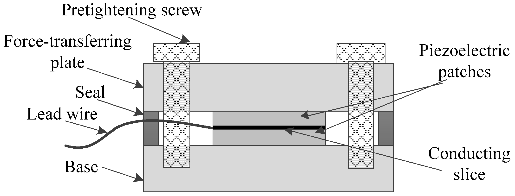
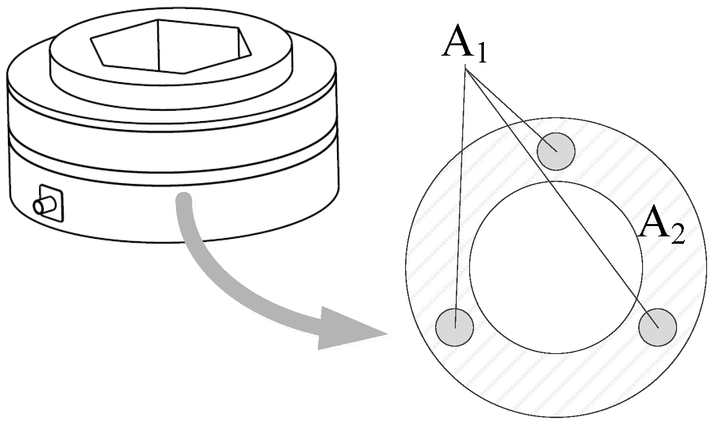
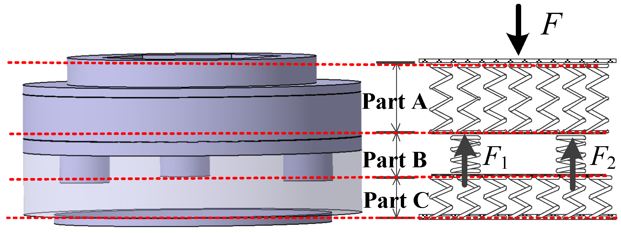
2.2. Key Techniques
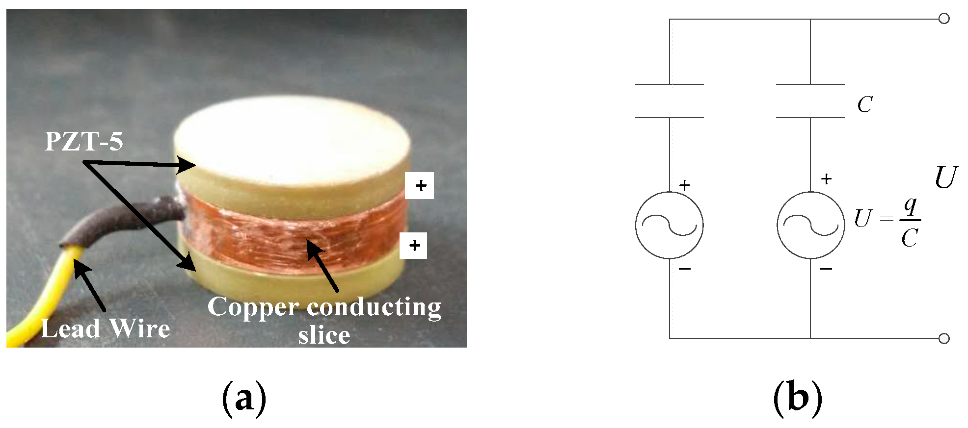
2.2.1. Theoretical Mechanism of Piezoelectric Sensors
2.2.2. Technique 1
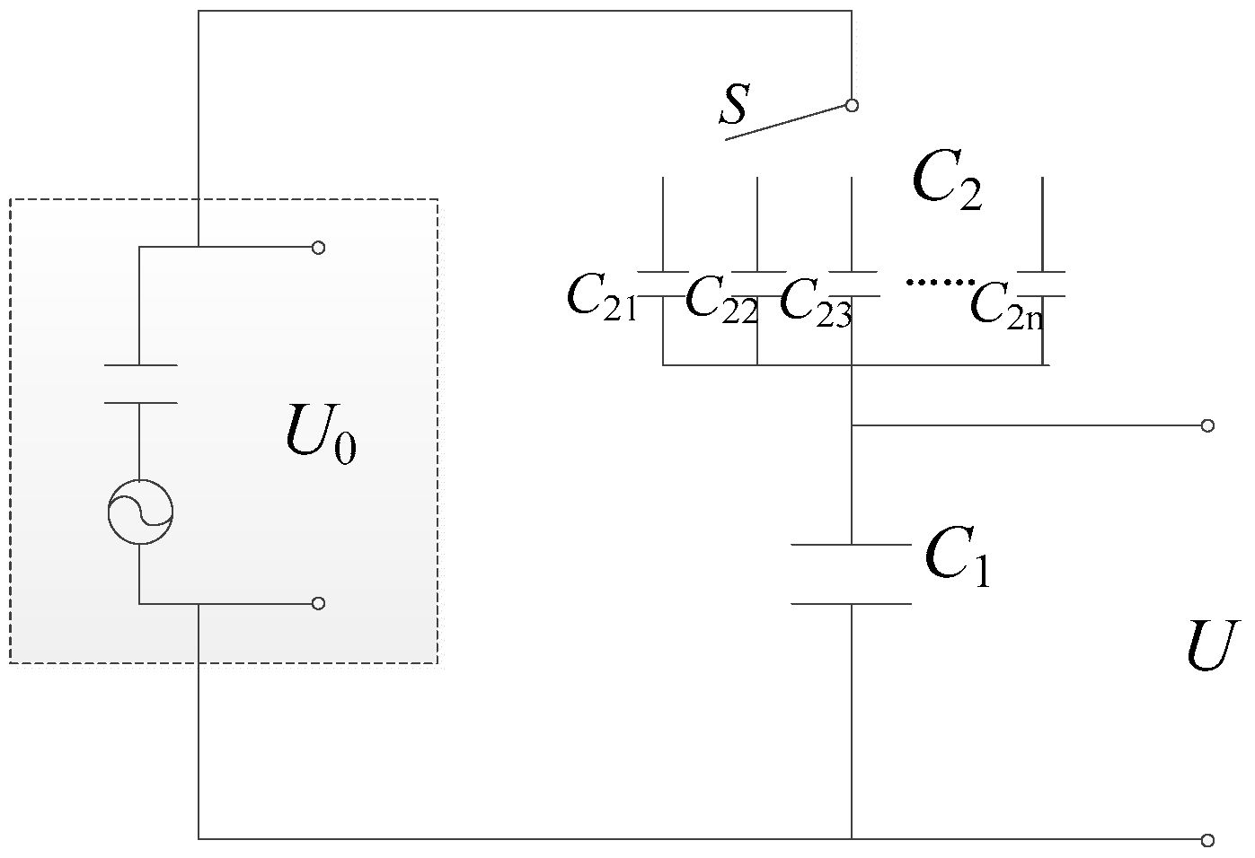
2.2.3. Technique 2
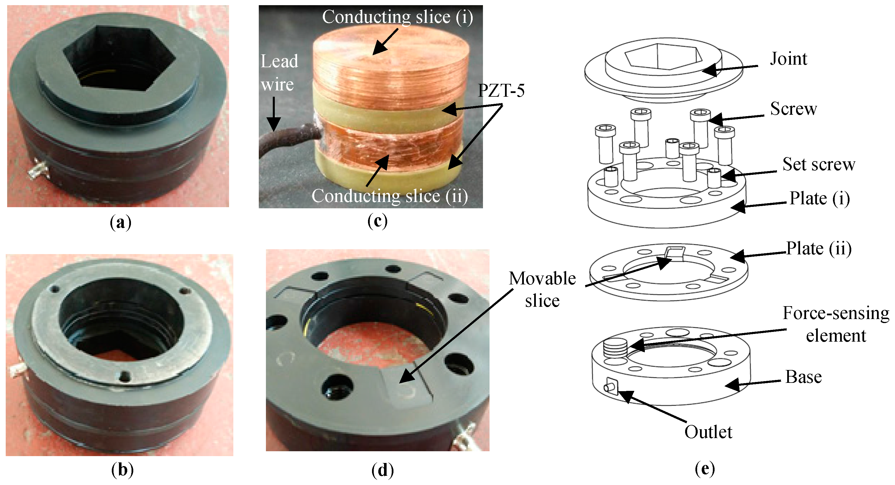
3. Assembly of the Sensor
4. Calibration Experiments
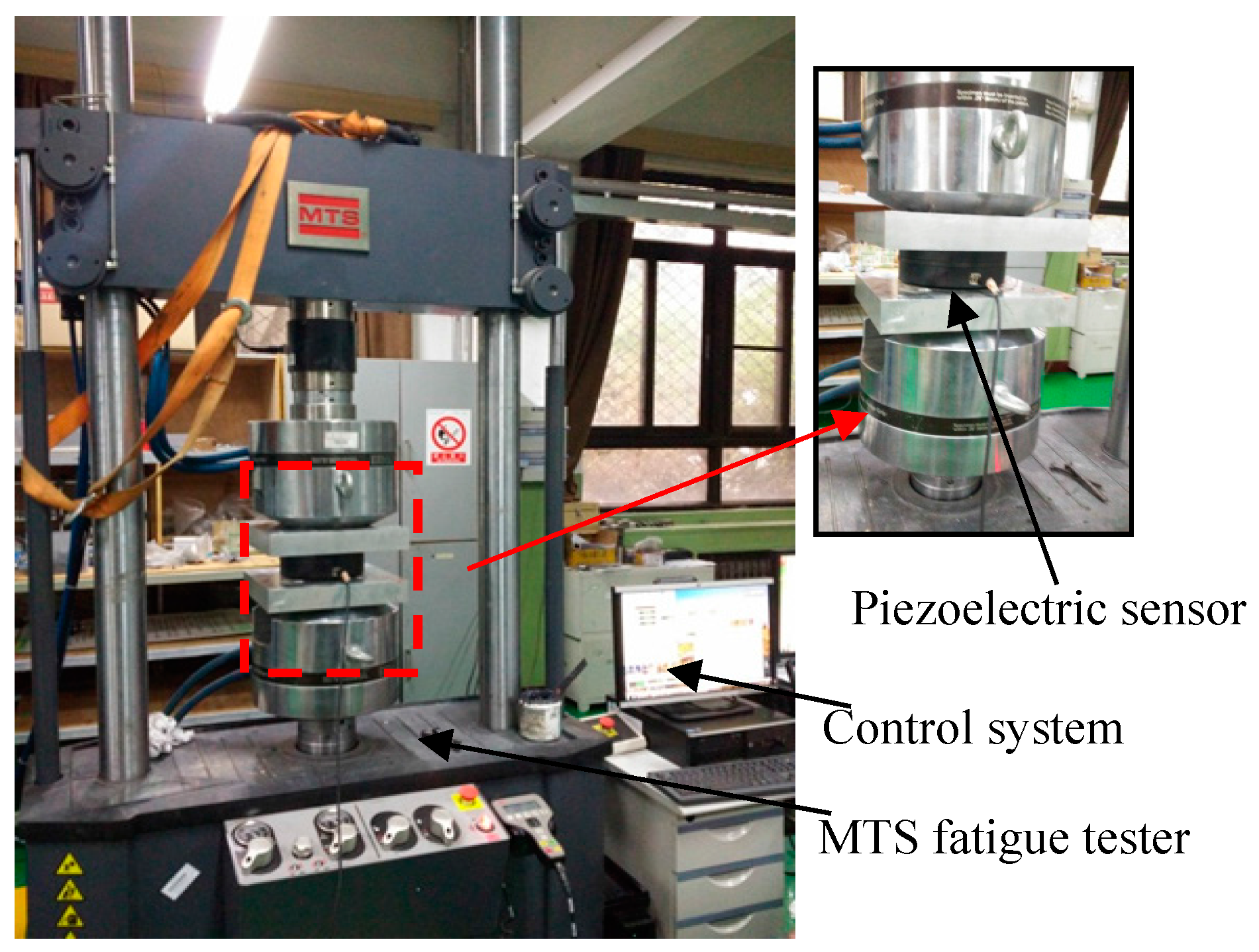
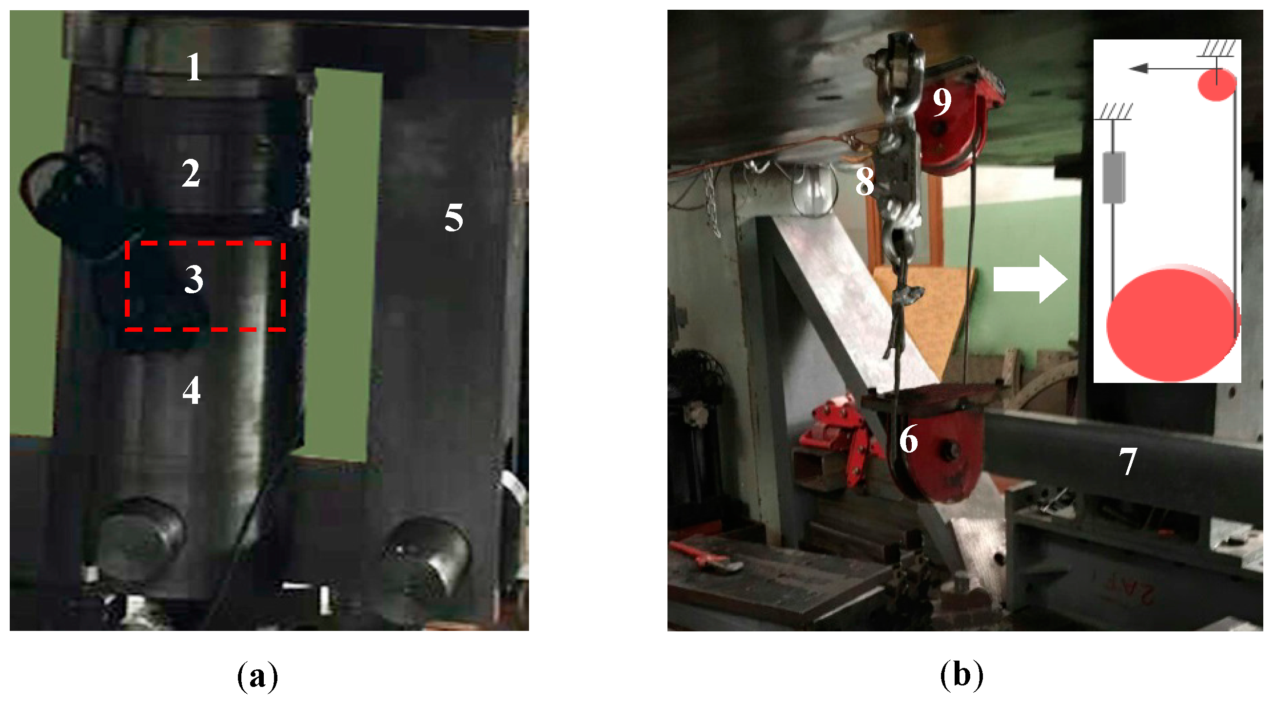
4.1. Experimental Setup
4.2. Experimental Scheme
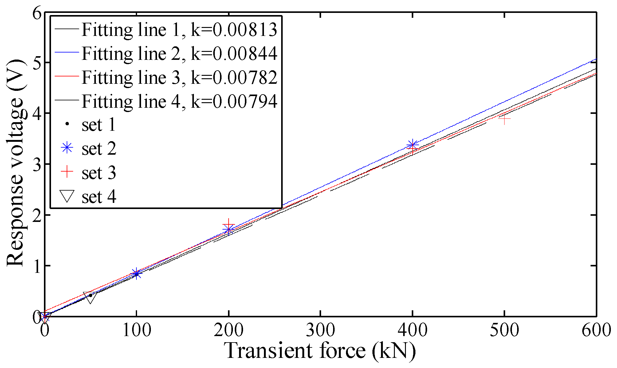
4.3. Experimental Results
5. Correction of Low-Frequency Measuring Signals
5.1. Low-Frequency Correction Principle
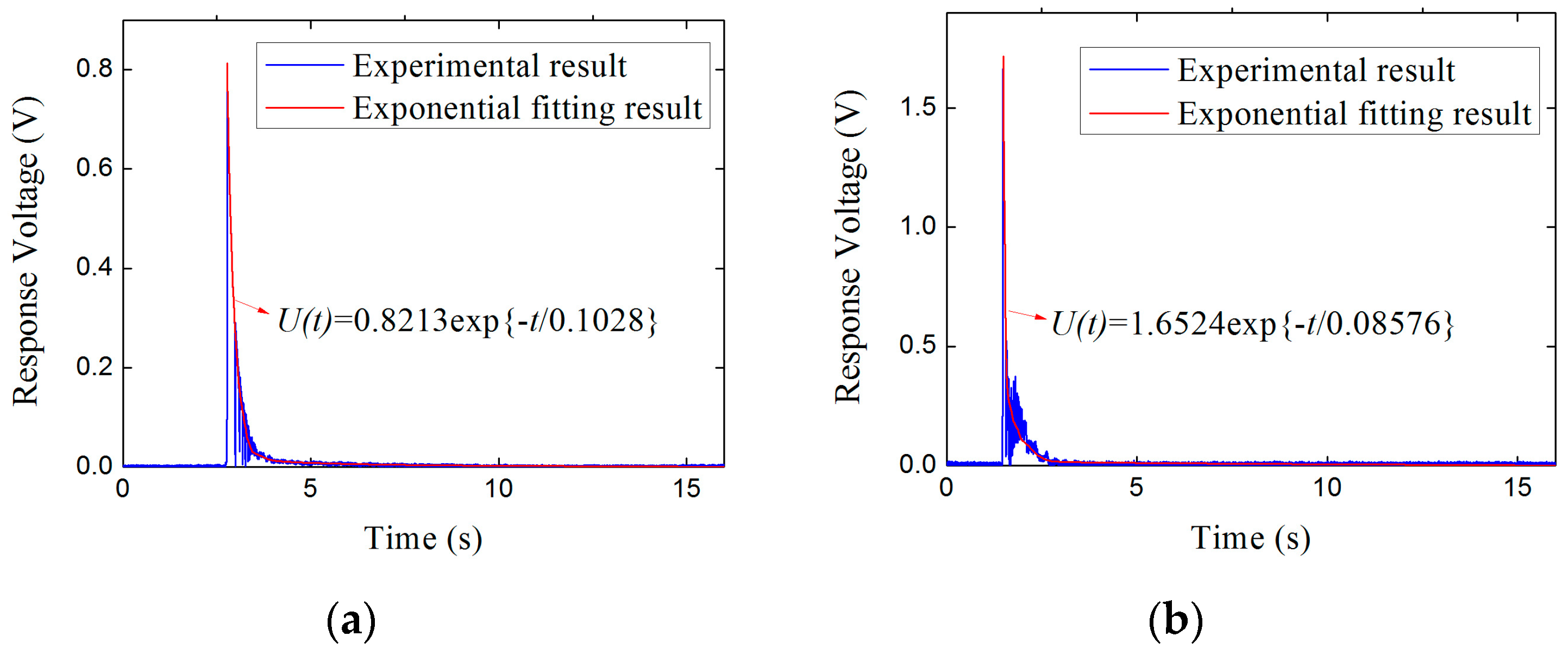
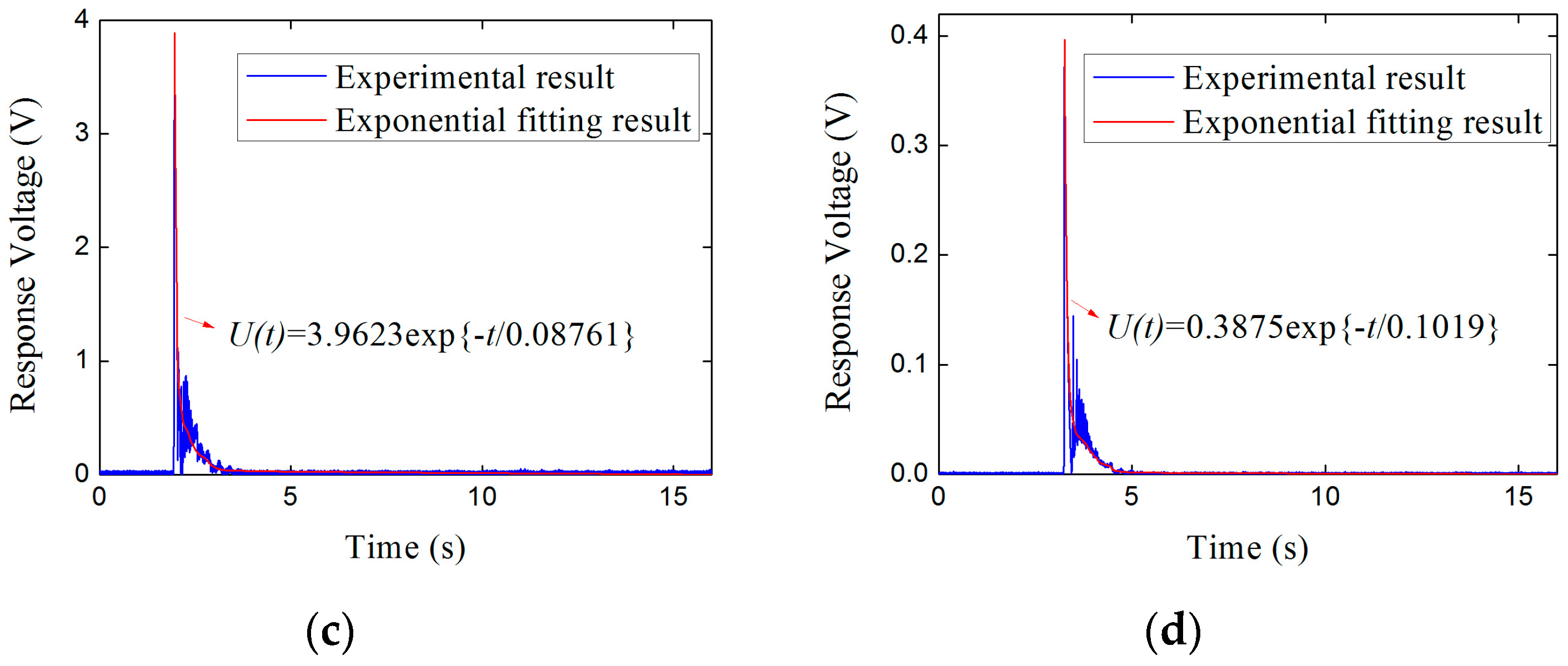
5.2. Parameter Identification of the Correction Function
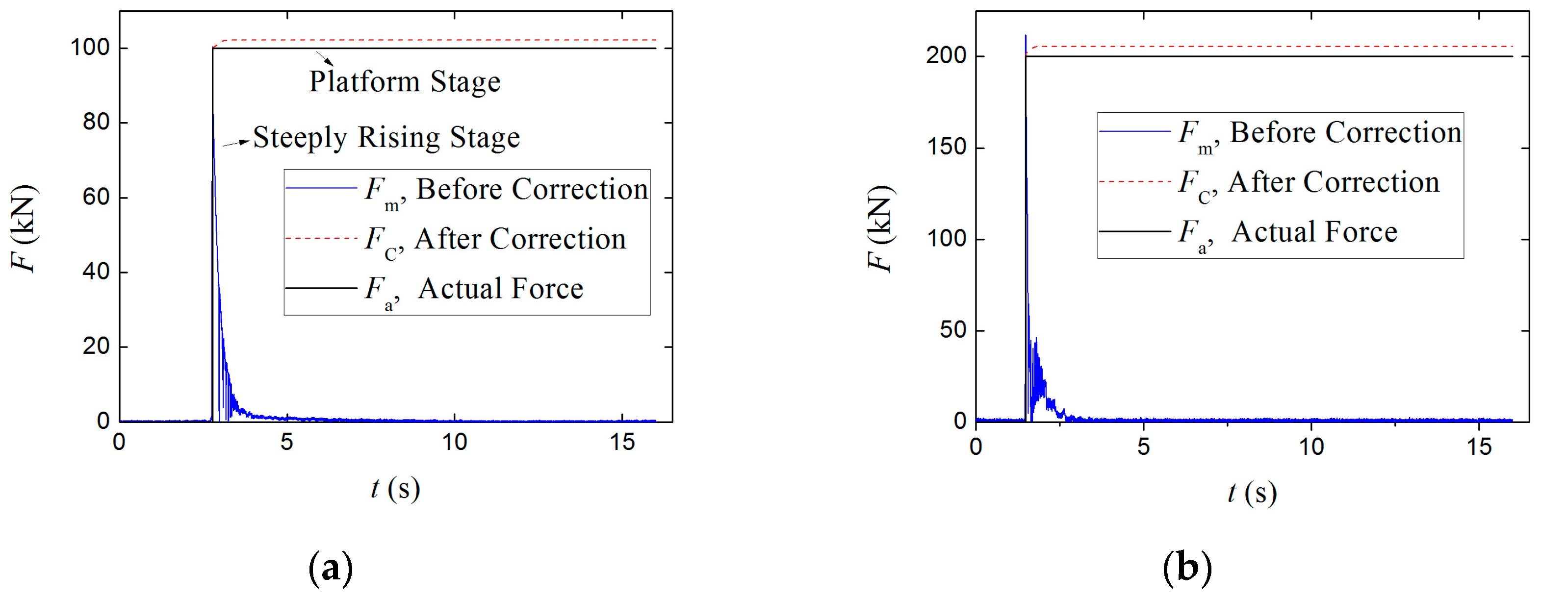
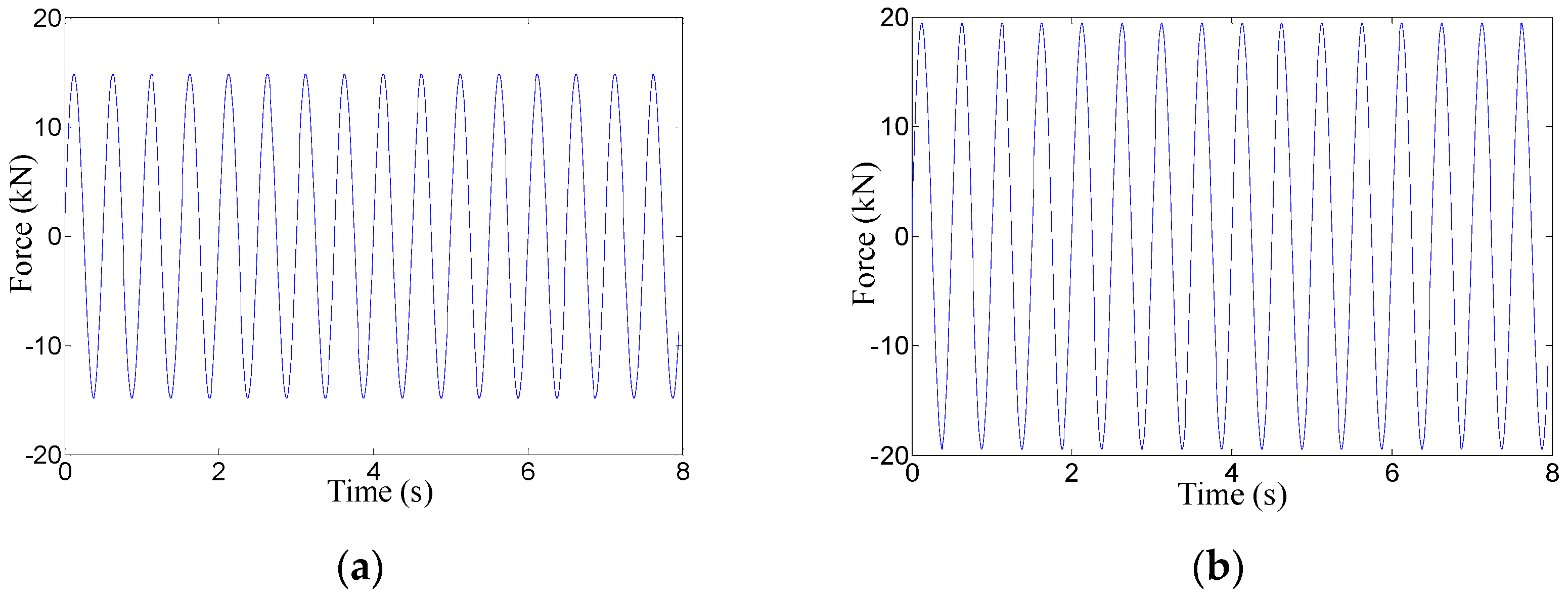
5.3. Experimental Verification of the Low-Frequency Correction Method
6. Conclusions
- (1)
- Two techniques of SSPDM and CCVDM are employed in the design of the sensor to satisfy the two prearranged static and dynamic indexes proposed based on the severe stress conditions in slope engineering. The SSPDM can greatly improve the compressive capacity (up to 1500 kN). The CCVDM can quantitatively decrease the high direct response voltage, by which the response signal of the sensor for the amplitude dynamic load of 500 kN can be collected.
- (2)
- The calibration experiments are conducted using the static and transient loading mechanism, which is independently developed employing the lever principle and can match the high loading requirements in practical engineering. Based on the experimental results, the sensitivity coefficient is obtained. The experimental results also reveal that the sensor has compressive capacity up to 1500 kN, stable sensitivities under different static preload levels and wide-range dynamic measuring linearity from 0 to 500 kN.
- (3)
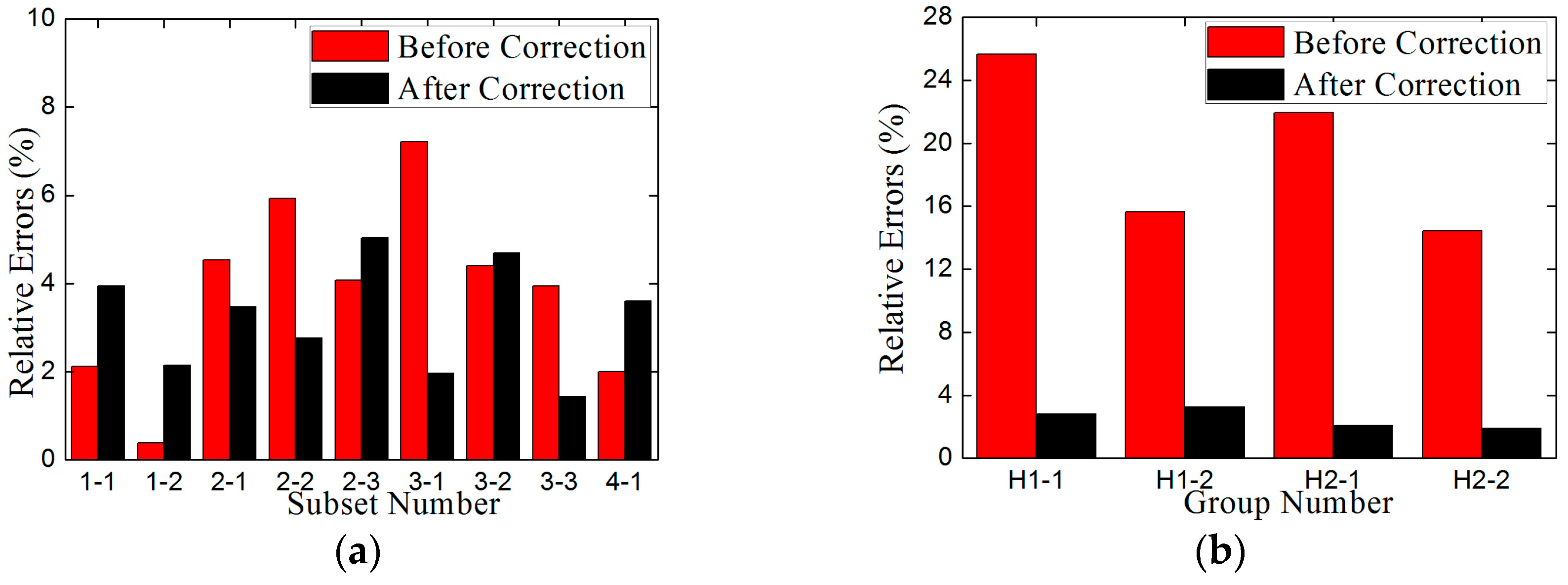
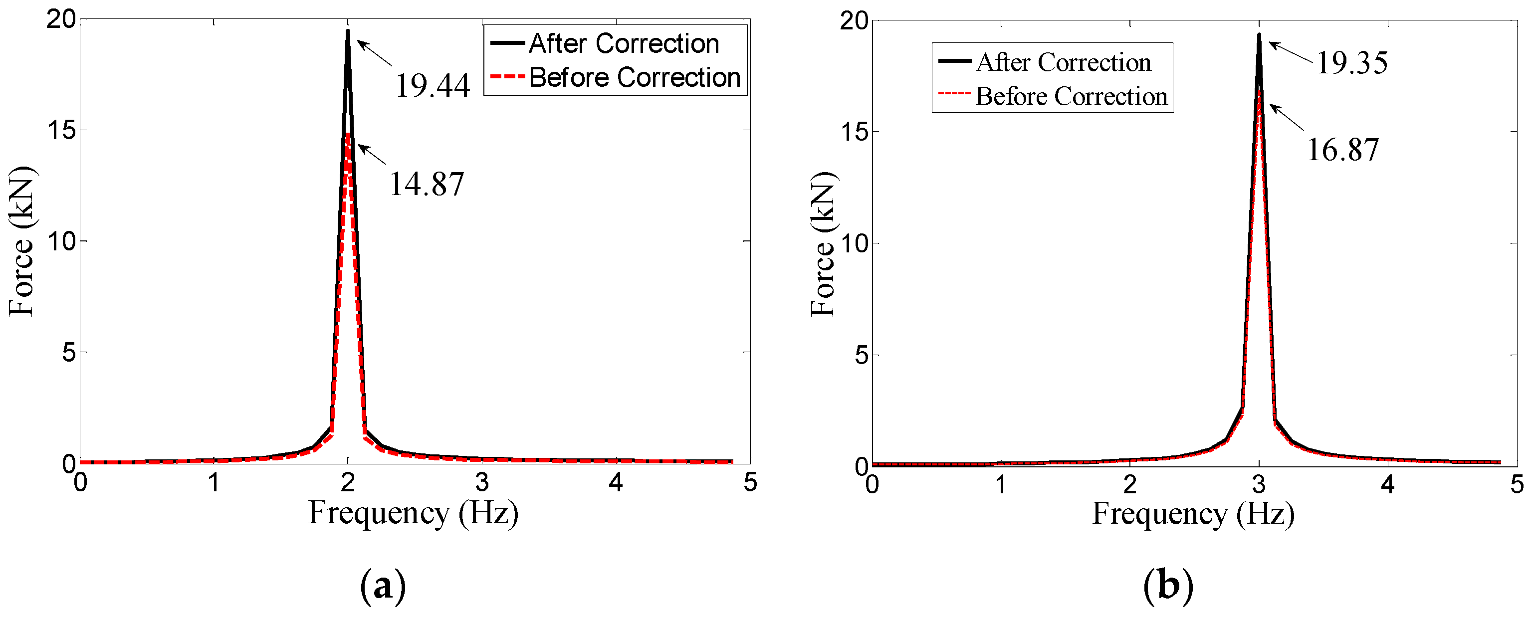
- The low-frequency correction method for the piezoelectric sensor is proposed and experimentally verified by imposing the step force and low-frequency harmonic force with different amplitudes on the sensor. The results reveal that the relative errors after correction are much lower than those before correction. Thus, low-frequency measuring reliability of the piezoelectric sensor is effectively improved.
Author Contributions
Conflicts of Interest
References
- Romeo, R.W.; Floris, M.; Veneri, F. Area-scale landslide hazard and risk assessment. Environ. Geol. 2006, 51, 1–13. [Google Scholar] [CrossRef]
- Kamai, T. Monitoring the process of ground failure in repeated landslides and associated stability assessments. Environ. Geol. 1998, 50, 71–84. [Google Scholar] [CrossRef]
- Xu, L.K.; Li, S.H.; Liu, X.Y.; Feng, C. Application of real-time telemetry technology to landslide in Tianchi Fengjie of Three Gorges reservoir region. Chin. J. Rock. Mech. Eng. 2007, 26, 4477–4483. [Google Scholar]
- Zan, L.; Latini, G.; Piscina, E.; Polloni, G.; Baldelli, P. Landslides early warning monitoring system. Geoscience and Remote Sensing Symposium. In Proceedings of the IEEE International Geoscience and Remote Sensing Symposium, Toronto, ON, Canada, 24–28 June 2002.
- Reeves, B.A.; Stickley, G.F.; Noon, D.A.; Longstaff, I.D. Developments in monitoring mine slope stability using radar interferometry. Geoscience and Remote Sensing Symposium. In Proceedings of the IEEE 2000 International Geoscience and Remote Sensing Symposium. Taking the Pulse of the Planet: The Role of Remote Sensing in Managing the Environment, Honolulu, HI, USA, 24–28 July 2000.
- Puglisi, G.; Bonaccorso, A.; Mattia, M.; Aloisi, M.; Bonforte, A.; Campisi, O.; Cantarero, M.; Falzone, G.; Puglisi, B.; Rossi, M. New integrated geodetic monitoring system at Stromboli volcano (Italy). Eng. Geol. 2005, 79, 13–31. [Google Scholar] [CrossRef]
- Zhang, Y.; Li, H.; Sheng, Q.; Wu, K.; Chen, G. Real time remote monitoring and pre-warning system for Highway landslide in mountain area. J. Environ. Sci.-China 2011, 23, S100–S105. [Google Scholar] [CrossRef]
- Wu, K.; Sheng, Q.; Zhang, Y.H.; Li, Z.Y.; Li, H.X.; Yue, Z.P. Development of real-time remote monitoring and forecasting system for geological disasters at subgrade slopes of mountainous highways and its application. Rock. Soil. Mech. 2010, 31, 3683–3687. [Google Scholar]
- Perski, Z.; Hanssen, R.; Wojcik, A.; Wojciechowski, T. InSAR analyses of terrain deformation near the Wieliczka Salt Mine, Poland. Eng. Geol. 2009, 106, 58–67. [Google Scholar] [CrossRef]
- Jia, G.; Tian, Y.; Liu, Y.; Zhang, Y. A static and dynamic factors-coupled forecasting model of regional rainfall-induced landslides: A case study of Shenzhen. Sci. China Technol. Sci. 2008, 51, 164–175. [Google Scholar] [CrossRef]
- Xiang, Y.; Wang, L.; Wang, Z.J.; Yuan, H.; Guan, Y.J. Key techniques for evaluation of safety monitoring sensors in water conservancy and hydropower engineering. Water. Sci. Eng. 2012, 5, 440–449. [Google Scholar]
- Cochrane, C.; Koncar, V.; Lewandowski, M.; Dufour, C. Design and development of a flexible strain sensor for textile structures based on a conductive polymer composite. Sensors 2007, 7, 473–492. [Google Scholar] [CrossRef]
- Kuhinek, D.; Zoric, I. Enhanced Vibrating Wire Strain Sensor. In Proceedings of the 2007 IEEE Instrumentation and Measurement Technology Conference, Warsaw, Poland, 1–3 May 2007.
- Bourquin, F.; Joly, M. A magnet-based vibrating wire sensor: design and simulation. Smart. Mater. Struct. 2004, 14, 247. [Google Scholar] [CrossRef]
- Wang, Q.; Jiang, J.; Sun, Y.; Qi, Y.; Zhang, J.; Yin, F.; Li, Z. Research and development on high performance anchor cable dynamometric system based on vibrating-wire sensor technology. Chin. J. Rock. Mech. Eng. 2012, 31, 3981–3987. [Google Scholar]
- Agioutantis, Z.; Kaklis, K.; Mavrigiannakis, S.; Verigakis, M.; Vallianatos, F.; Saltas, V. Potential of acoustic emissions from three point bending tests as rock failure precursors. Int. J. Min. Sci. Technol. 2016, 26, 155–160. [Google Scholar] [CrossRef]
- Karayannis, C.G.; Chalioris, C.E.; Angeli, G.M.; Papadopoulos, N.A.; Favvata, M.J.; Providakis, C.P. Experimental damage evaluation of reinforced concrete steel bars using piezoelectric sensors. Constr. Build. Mater. 2016, 105, 227–244. [Google Scholar] [CrossRef]
- Yan, W.; Chen, W. Electro-mechanical response of functionally graded beams with imperfectly integrated surface piezoelectric layers. Sci. China Phys. Mech. 2006, 49, 513–525. [Google Scholar] [CrossRef]
- Yang, C.; Lu, Z. An interval effective independence method for optimal sensor placement based on non-probabilistic approach. Sci. China Technol. Sci. 2016, 60, 186–198. [Google Scholar] [CrossRef]
- Yang, C.; Hou, X.; Wang, L.; Zhang, X. Applications of different criteria in structural damage identification based on natural frequency and static displacement. Sci. China Technol. Sci. 2016, 59, 1746–1758. [Google Scholar] [CrossRef]
- Gu, H.; Moslehy, Y.; Sanders, D.; Song, G.; Mo, Y.L. Multi-functional smart aggregate-based structural health monitoring of circular reinforced concrete columns subjected to seismic excitations. Smart. Mater. Struct. 2010, 19, 065026. [Google Scholar] [CrossRef]
- Chalioris, C.E.; Papadopoulos, N.A.; Angeli, G.M.; Karayannis, C.G.; Liolios, A.A.; Providakis, C.P. Damage evaluation in shear-critical reinforced concrete beam using piezoelectric transducers as smart aggregates. Open. Eng. 2015, 1, 373–384. [Google Scholar] [CrossRef]
- Voutetaki, M.E.; Papadopoulos, N.A.; Angeli, G.M.; Providakis, C.P. Investigation of a new experimental method for damage assessment of RC beams failing in shear using piezoelectric transducers. Eng. Struct. 2016, 114, 226–240. [Google Scholar] [CrossRef]
- He, M.C. Real-time remote monitoring and forecasting system for geological disasters of landslides and its engineering application. Chin. J. Rock. Mech. Eng. 2009, 28, 1081–1090. [Google Scholar]
- He, M.C.; Tao, Z.G.; Zhang, B. Application of remote monitoring technology in landslides in the Luoshan mining area. Int. J. Min. Sci. Technol. 2009, 19, 609–614. [Google Scholar] [CrossRef]
- He, M.; Gong, W.; Wang, J.; Qi, P.; Tao, Z.; Du, S.; Peng, Y. Development of a novel energy-absorbing bolt with extraordinarily large elongation and constant resistance. Int. J. Rock. Mech. Min. Sci. 2014, 67, 29–42. [Google Scholar] [CrossRef]
- Tao, Z.G.; Li, H.P.; Sun, G.L. Development of monitoring and early warning system for landslides based on constant resistance and large deformation anchor cable and its application. Rock. Soil. Mech. 2015, 36, 3032–3040. [Google Scholar]
- Yang, X.; Hou, D.; Tao, Z.; Peng, Y.; Shi, H. Stability and remote real-time monitoring of the slope slide body in the Luoshan mining area. Int. J. Min. Sci. Technol. 2015, 25, 761–765. [Google Scholar] [CrossRef]
- Zhu, Y.P.; Kong, D.R.; Wang, F. Sensors Principles and Applications; National Defense Industry Press: Beijing, China, 2005; pp. 77–100. [Google Scholar]
- Chen, J.P.; Cheng, W.; Li, M. Low-frequency compensation method of piezoelectric force sensor and experimental verification. J. Vib. Meas. Diag. 2016, 36, 325–328. [Google Scholar]
- Chen, J.P.; Cheng, W. Low-frequency compensation of piezoelectric micro-vibration test platform. Tech. Vjesn. 2016, 23, 1251–1258. [Google Scholar]


| Parameter Name | Value | Units |
|---|---|---|
| Electrode surface area | 3.14 × 10⁻⁴ | m2 |
| Thickness | 0.003 | m |
| Density | 7.5 × 10³ | kg/m3 |
| Elastic modulus | 117 | GPa |
| Compressive strength | 76 | MPa |
| Piezoelectric constant | 4.15 × 10⁻⁷ | C/N |
| Relative dielectric constant | 2100 | - |
| Vacuum dielectric constant | 8.85 × 10⁻¹² | F/m |
| Parameter Name | Value | Units | |
|---|---|---|---|
| Vibration wire sensor | Outer diameter | 0.066 | m |
| Inner diameter | 0.111 | m | |
| Height | 0.1 | m | |
| Cable lockset | Diameter | 0.172 | m |
| Height | 0.06 | m | |
| Anchor cables | Outer diameter | 0.092 | m |
| Diameter (single cable) | 0.01524 | m | |
| Cable quantity | 6 | - | |
| Parameter Name | Value | Units | |
|---|---|---|---|
| Piezoelectric sensor | Outer diameter | 0.19 | m |
| Inner diameter | 0.11 | m | |
| Height | 0.073 | m | |
| Base | Thickness | 0.035 | m |
| Depth of cylindrical groove | 0.0155 | m | |
| Plate (i) | Thickness | 0.025 | m |
| Plate (ii) | Thickness | 0.008 | m |
| Basal area | 0.016 | m2 | |
| Moving slice | Thickness | 0.006 | m |
| Force-sensing element | Height | 0.016 | m |
| Copper conducting slice | Thickness | 0.005 | m |
| Elastic module | 100 | Gpa | |
| Steel (main body) | Elastic module | 210 | Gpa |
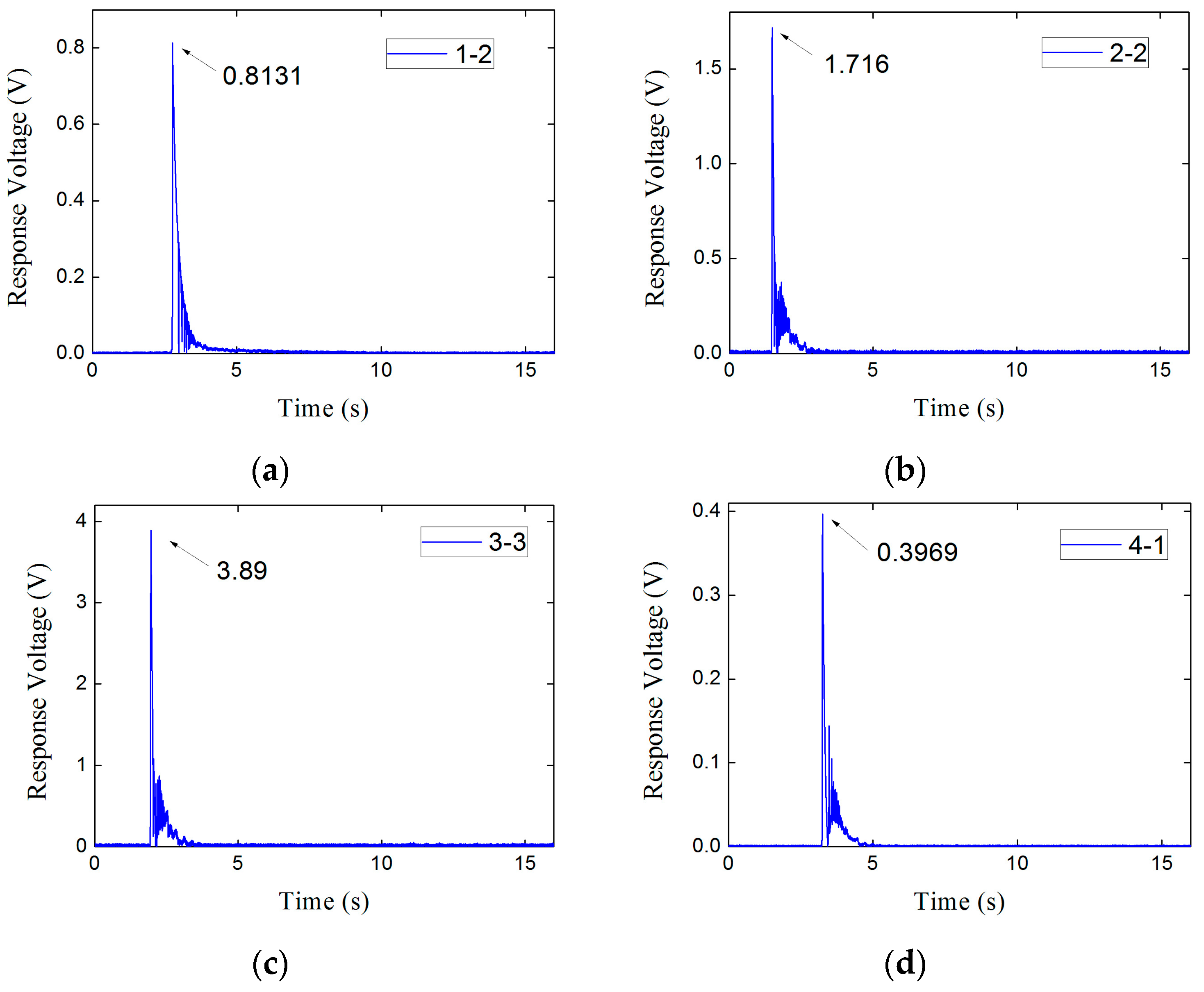
| Set | Static Preload/kN | Subset | Amplitude of Transient Step-Load/kN | Peak Response Voltage/V |
|---|---|---|---|---|
| 1 | 300 | 1-1 | 50 | 0.4163 |
| 1-2 | 100 | 0.8131 | ||
| 2 | 600 | 2-1 | 100 | 0.8467 |
| 2-2 | 200 | 1.716 | ||
| 2-3 | 400 | 3.372 | ||
| 3 | 1000 | 3-1 | 200 | 1.737 |
| 3-2 | 400 | 3.097 | ||
| 3-3 | 500 | 3.890 | ||
| 4 | 1500 | 4-1 | 50 | 0.3969 |
| Set | Subset | Amplitude of Fa/kN | Fm (Before Correction) | Fc (After Correction) | ||
|---|---|---|---|---|---|---|
| Amplitude/kN | Error | Amplitude/kN | Error | |||
| 1 | 1-1 | 50 | 51.06 | 2.12% | 51.97 | 3.94% |
| 1-2 | 100 | 100.38 | 0.38% | 102.15 | 2.15% | |
| 2 | 2-1 | 100 | 104.53 | 4.53% | 103.47 | 3.47% |
| 2-2 | 200 | 211.85 | 5.93% | 205.52 | 2.76% | |
| 2-3 | 400 | 416.3 | 4.08% | 379.88 | 5.03% | |
| 3 | 3-1 | 200 | 214.44 | 7.22% | 203.92 | 1.96% |
| 3-2 | 400 | 382.35 | 4.41% | 381.24 | 4.69% | |
| 3-3 | 500 | 480.25 | 3.95% | 492.82 | 1.44% | |
| 4 | 4-1 | 50 | 49 | 2% | 48.2 | 3.61% |
| No. | Static Pre-load/kN | Fa (Harmonic Force) | Fm (Before Correction) | Fc (After Correction) | |||
|---|---|---|---|---|---|---|---|
| Amplitude/kN | Frequency/Hz | Amplitude/kN | Error | Amplitude/kN | Error | ||
| H1-1 | 100 | 20 | 2 | 14.87 | 25.65% | 19.44 | 2.8% |
| H1-2 | 100 | 20 | 3 | 16.87 | 15.65% | 19.35 | 3.25% |
| H2-1 | 100 | 40 | 2 | 31.23 | 21.93% | 40.83 | 2.08% |
| H2-2 | 100 | 40 | 3 | 34.23 | 14.43% | 39.25 | 1.9% |
© 2017 by the authors. Licensee MDPI, Basel, Switzerland. This article is an open access article distributed under the terms and conditions of the Creative Commons Attribution (CC BY) license ( http://creativecommons.org/licenses/by/4.0/).
Share and Cite
Li, M.; Cheng, W.; Chen, J.; Xie, R.; Li, X. A High Performance Piezoelectric Sensor for Dynamic Force Monitoring of Landslide. Sensors 2017, 17, 394. https://doi.org/10.3390/s17020394
Li M, Cheng W, Chen J, Xie R, Li X. A High Performance Piezoelectric Sensor for Dynamic Force Monitoring of Landslide. Sensors. 2017; 17(2):394. https://doi.org/10.3390/s17020394
Chicago/Turabian StyleLi, Ming, Wei Cheng, Jiangpan Chen, Ruili Xie, and Xiongfei Li. 2017. "A High Performance Piezoelectric Sensor for Dynamic Force Monitoring of Landslide" Sensors 17, no. 2: 394. https://doi.org/10.3390/s17020394
APA StyleLi, M., Cheng, W., Chen, J., Xie, R., & Li, X. (2017). A High Performance Piezoelectric Sensor for Dynamic Force Monitoring of Landslide. Sensors, 17(2), 394. https://doi.org/10.3390/s17020394