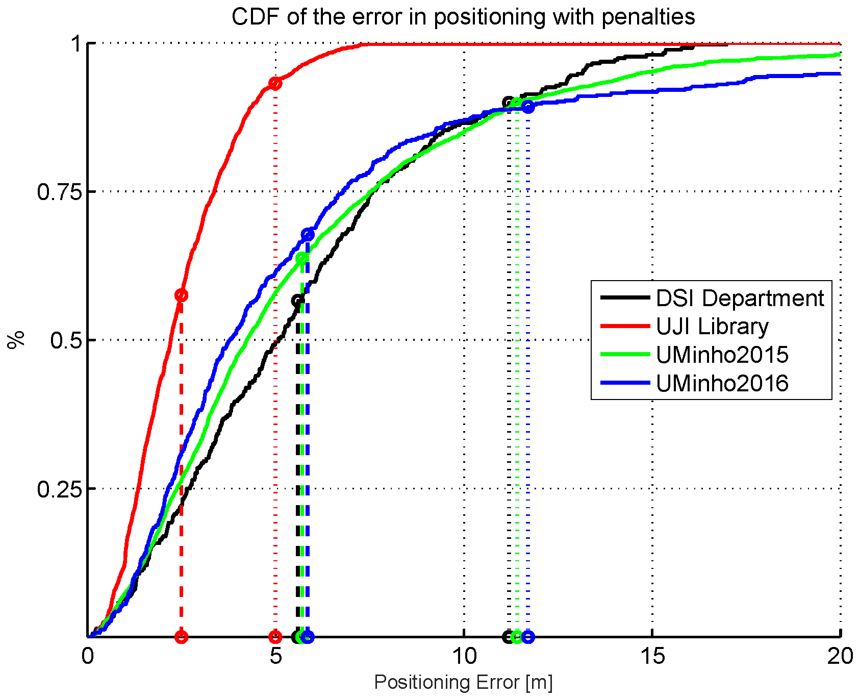
Figure 1.
Cumulative distribution of the positioning error (CDF) for four different cases. Simple Wi-Fi fingerprinting system based on kNN at the DSI department (University of Minho, Portugal); Simple Wi-Fi fingerprinting system based on kNN at a small area of the university library building (Universiat Jaume I, Spain); UMinho system at the 2015 IPIN competition; UMinho system at the 2016 IPIN competition. The errors and penalties in floor detection are not considered in any of the results shown. Dashed vertical lines indicate the average error, whereas dotted vertical lines indicate twice the average error.
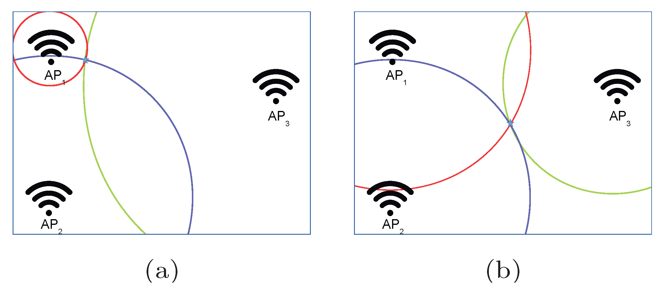
Figure 2.
Illustrative examples of the areas where a fingerprint can be placed in the optimistic world. (a) Fingerprint placed near to . (b) Fingerprint equidistant to all APs.
Figure 2.
Illustrative examples of the areas where a fingerprint can be placed in the optimistic world. (a) Fingerprint placed near to . (b) Fingerprint equidistant to all APs.
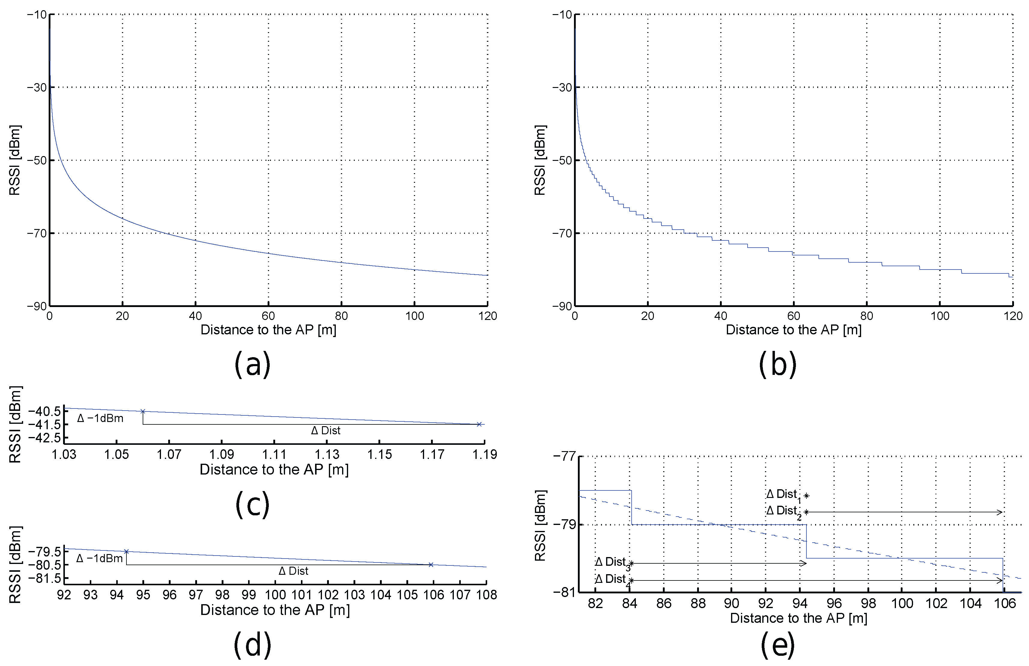
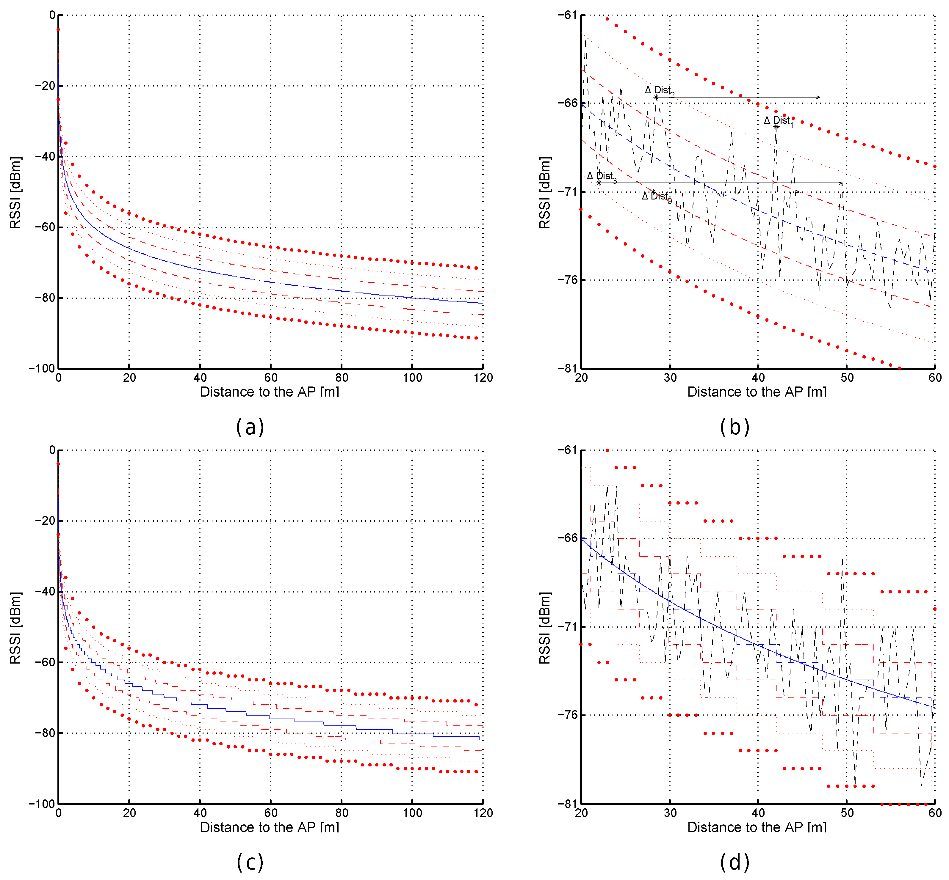
Figure 3.
Received signal strength intensities (RSSI) against distance for optimistic (a) and quantized (b) worlds. (c,d) Excerpts of (a). (e) Excerpt of (b).
Figure 3.
Received signal strength intensities (RSSI) against distance for optimistic (a) and quantized (b) worlds. (c,d) Excerpts of (a). (e) Excerpt of (b).
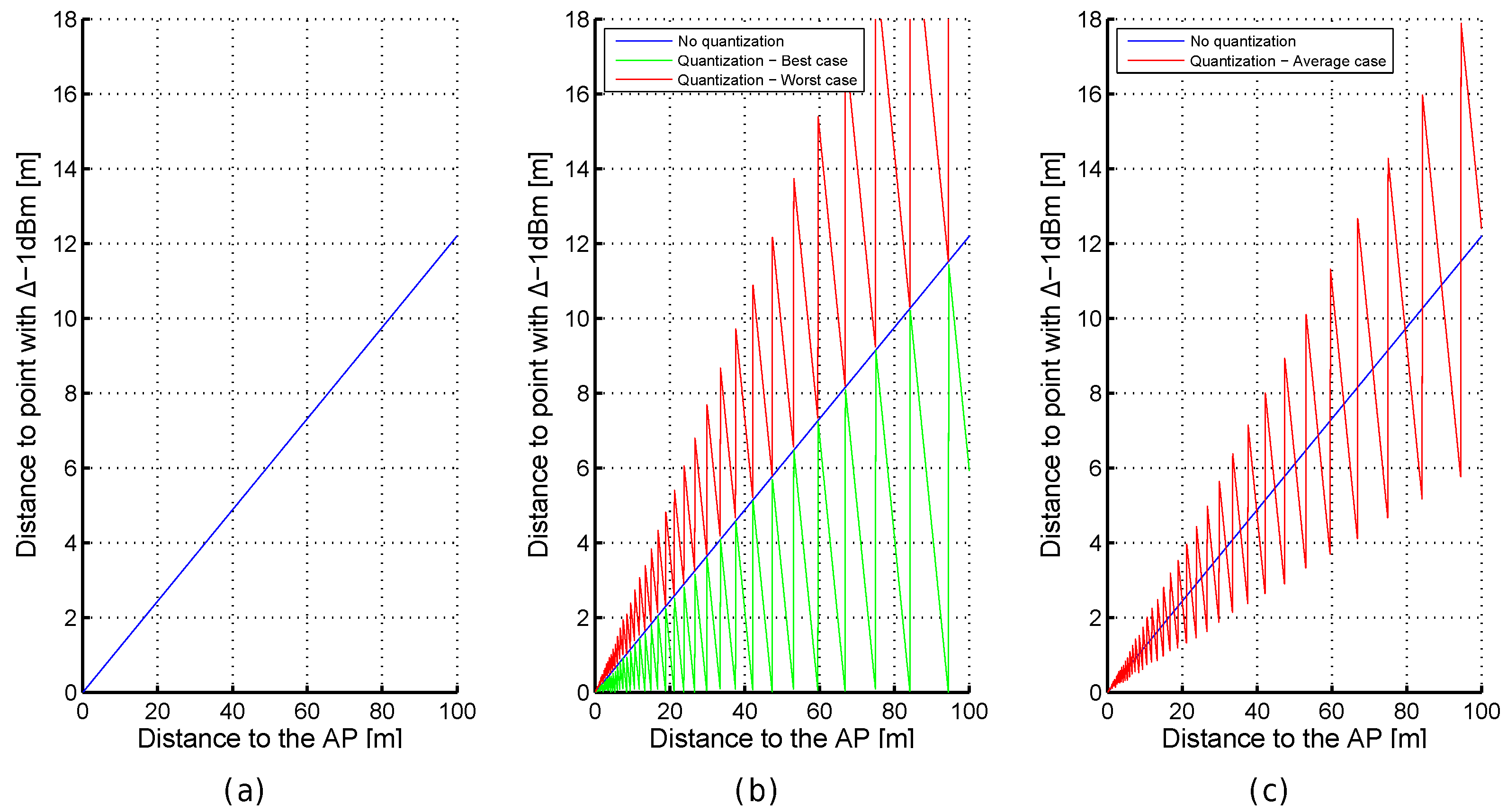
Figure 4.
Importance of dBm in the. optimistic (a) and quantized (b,c) worlds
Figure 4.
Importance of dBm in the. optimistic (a) and quantized (b,c) worlds
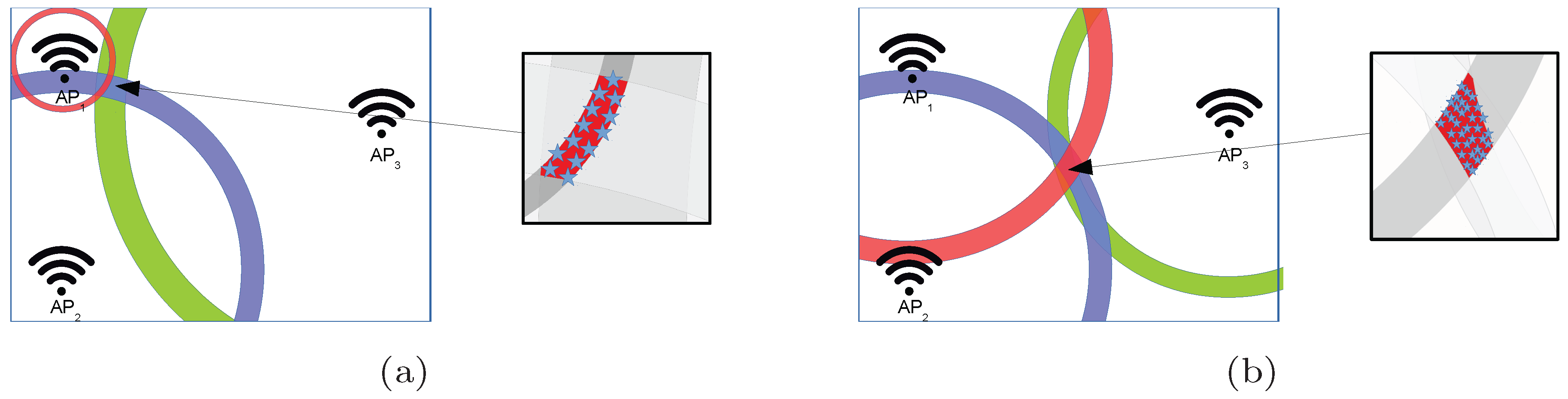
Figure 5.
Illustrative examples of the areas where a fingerprint can be placed in the quantized world. (a) Fingerprint placed near . (b) Fingerprint equidistant to all APs.
Figure 5.
Illustrative examples of the areas where a fingerprint can be placed in the quantized world. (a) Fingerprint placed near . (b) Fingerprint equidistant to all APs.
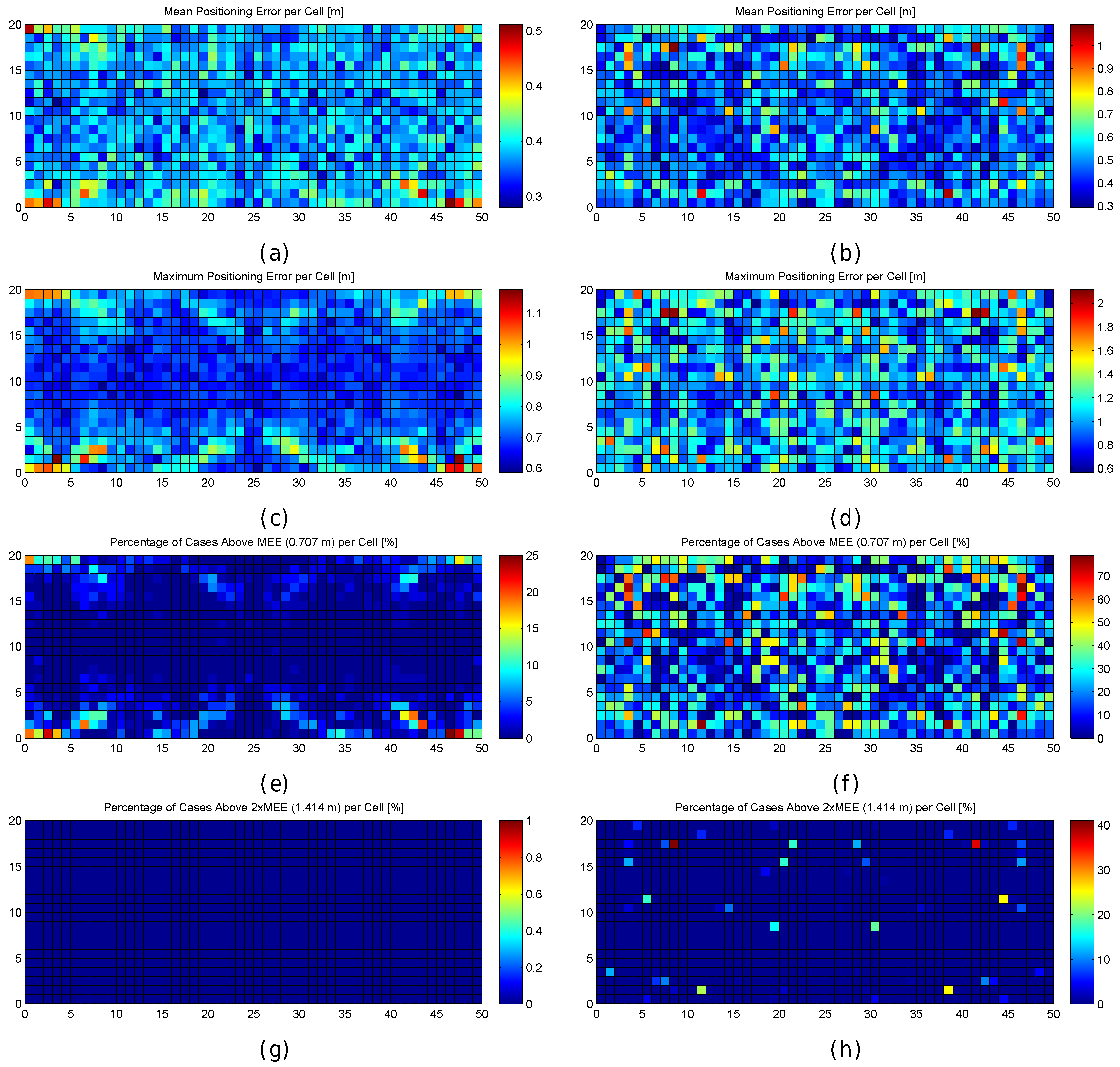
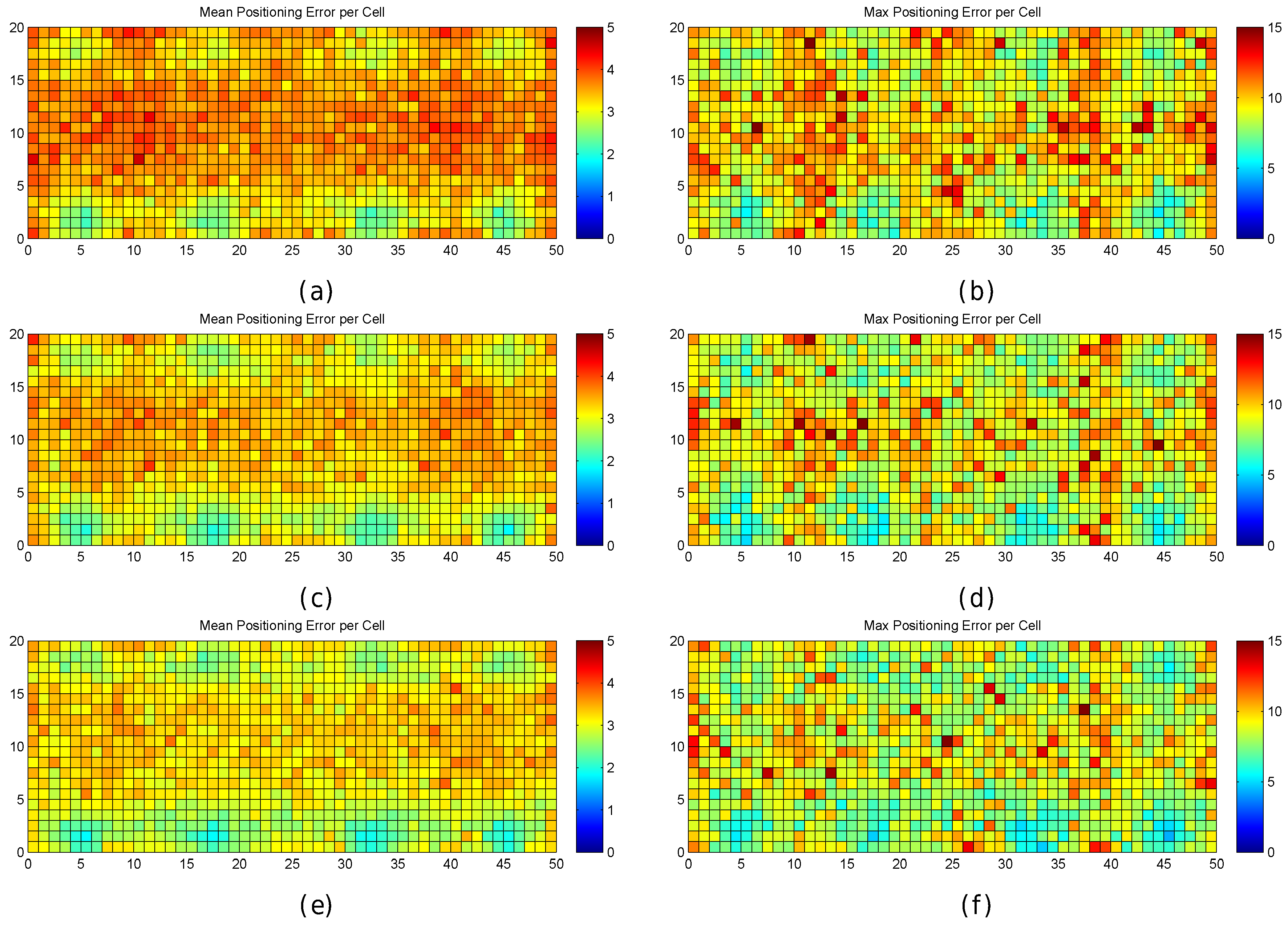
Figure 6.
Graphical results for analysing the impact of quantization. (a,b) mean positioning error per cell in the optimistic and quantized worlds respectively; (c,d) maximum positioning error per cell in the optimistic and quantized worlds respectively; (e,f) percentage of cases where the error was higher than MEE per cell in the optimistic and quantized worlds respectively; (g,h) percentage of cases where the error was higher than twice the MEE per cell in the optimistic and quantized worlds respectively.
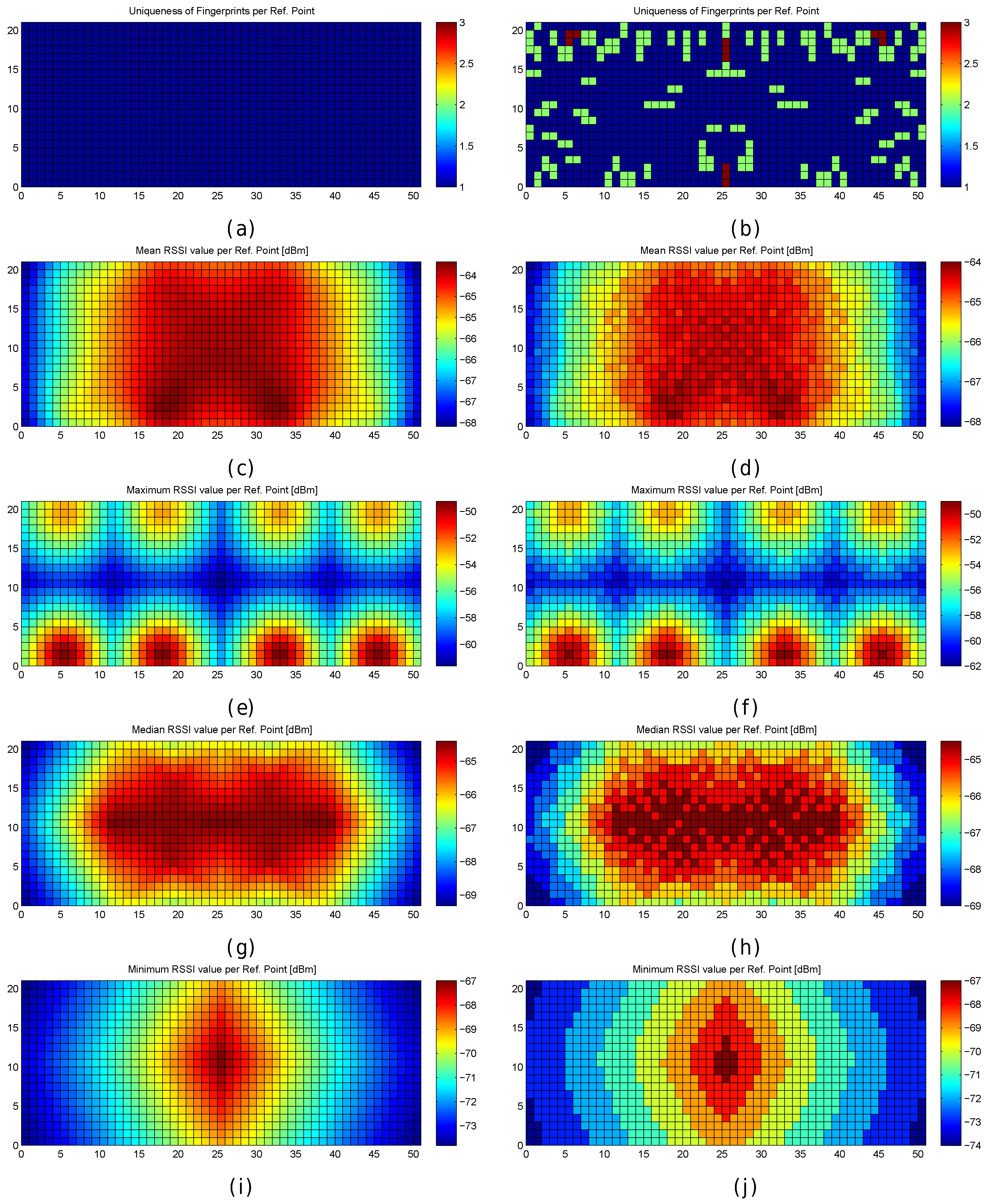
Figure 7.
RSSI and fingerprint statistics in the optimistic world (left images) and quantized world (right images). (a,b) uniqueness of reference fingerprints; (c,d) mean RSSI value of reference fingerprints; (e,f) maximum RSSI value of reference fingerprints; (g,h) median RSSI value of reference fingerprints; (i,j) minimum RSSI value of reference fingerprints.
Figure 8.
Received signal strength intensities (RSSI) against distance for the realistic noisy world () without quantization (a) and with quantization (c). (b) Excerpt of (a). (d) Excerpt of (c).
Figure 8.
Received signal strength intensities (RSSI) against distance for the realistic noisy world () without quantization (a) and with quantization (c). (b) Excerpt of (a). (d) Excerpt of (c).
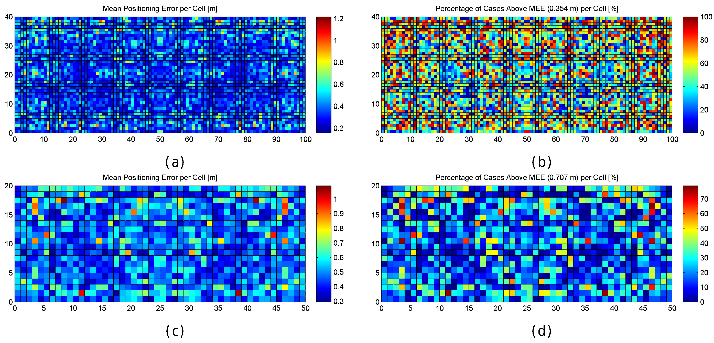
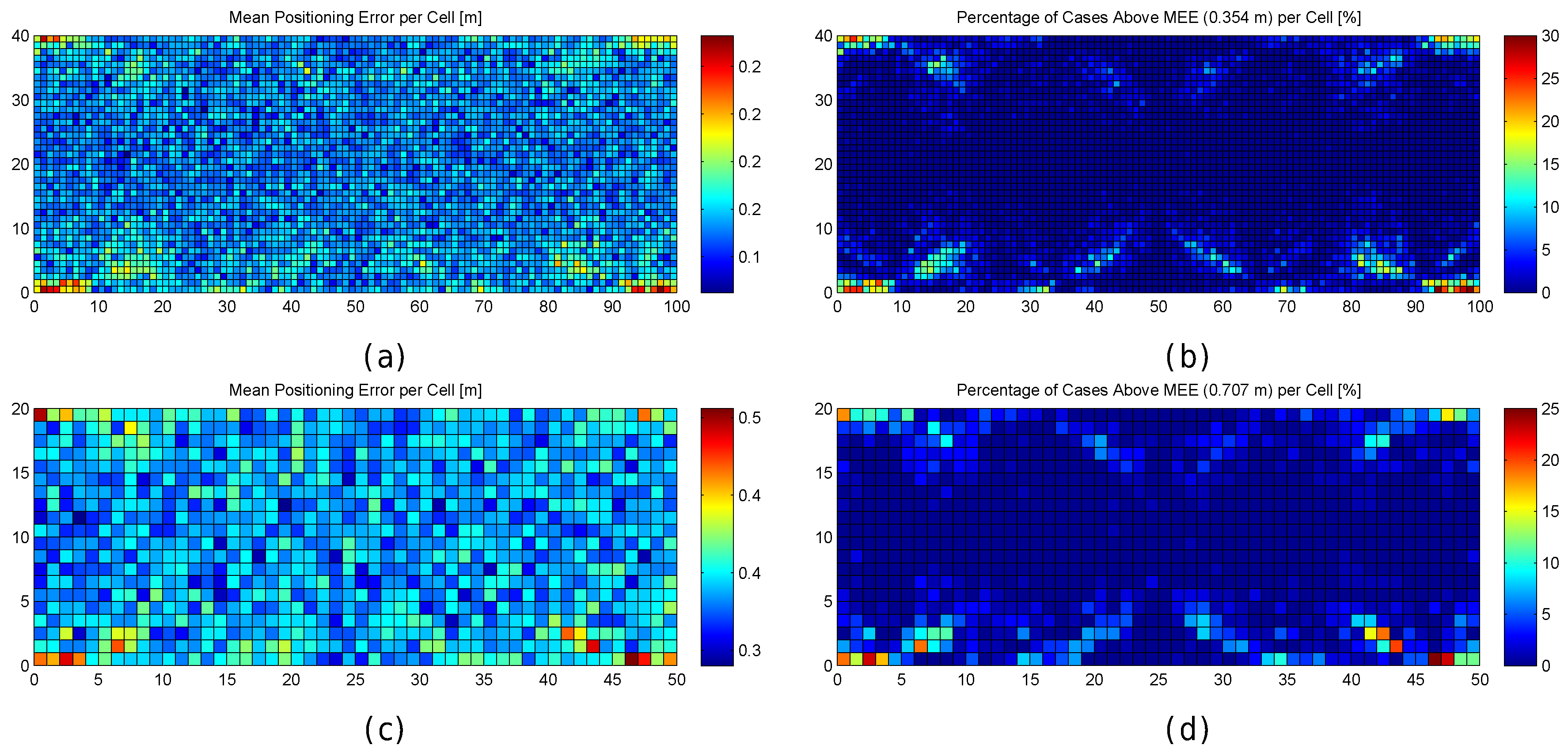
Figure 9.
Graphical results for analysing the grid size in the optimistic world. (a,c) mean positioning error per cell in the optimistic world for a grid size of 0.5 m and 1 m respectively; (b,d) percentage of cases where the positioning error is above the MEE for a grid size of 0.5 m and 1 m respectively.
Figure 10.
Graphical results for analysing the grid size in the quantized world. (a,c) mean positioning error per cell in the quantized world for a grid size of 0.5 m and 1 m respectively; (b,d) percentage of cases above the MEE in the quantized world for a grid size of 0.5 m and 1 m respectively.
Figure 10.
Graphical results for analysing the grid size in the quantized world. (a,c) mean positioning error per cell in the quantized world for a grid size of 0.5 m and 1 m respectively; (b,d) percentage of cases above the MEE in the quantized world for a grid size of 0.5 m and 1 m respectively.
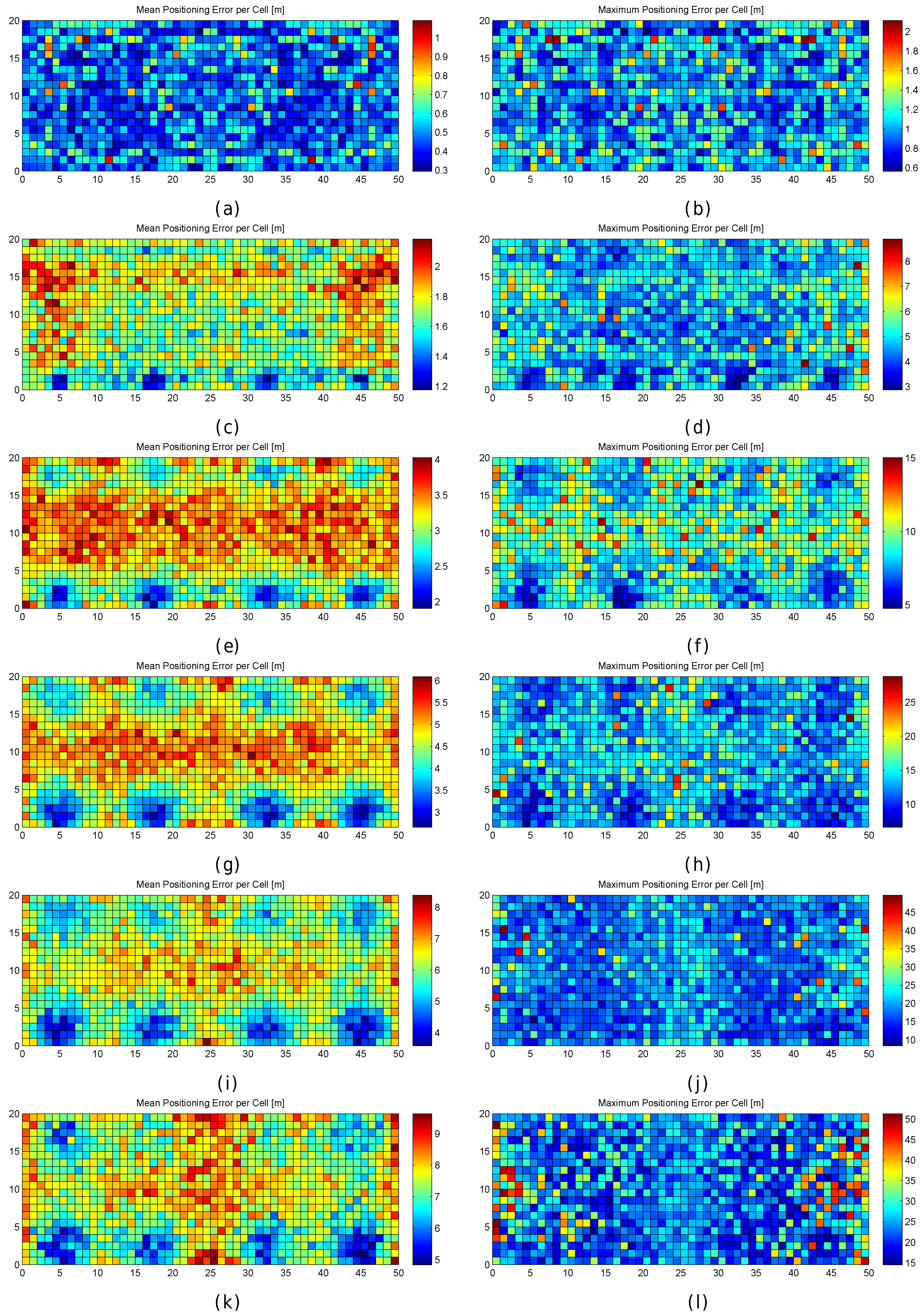
Figure 11.
Graphical results (mean and maximum positioning errors over 100 runs) for analysing the grid size in the noisy world. (a,b) results for (no noise); (c,d) results for ; (e,f) results for ; (g,h) results for ; (i,j) results for ; (k,l) results for .
Figure 11.
Graphical results (mean and maximum positioning errors over 100 runs) for analysing the grid size in the noisy world. (a,b) results for (no noise); (c,d) results for ; (e,f) results for ; (g,h) results for ; (i,j) results for ; (k,l) results for .
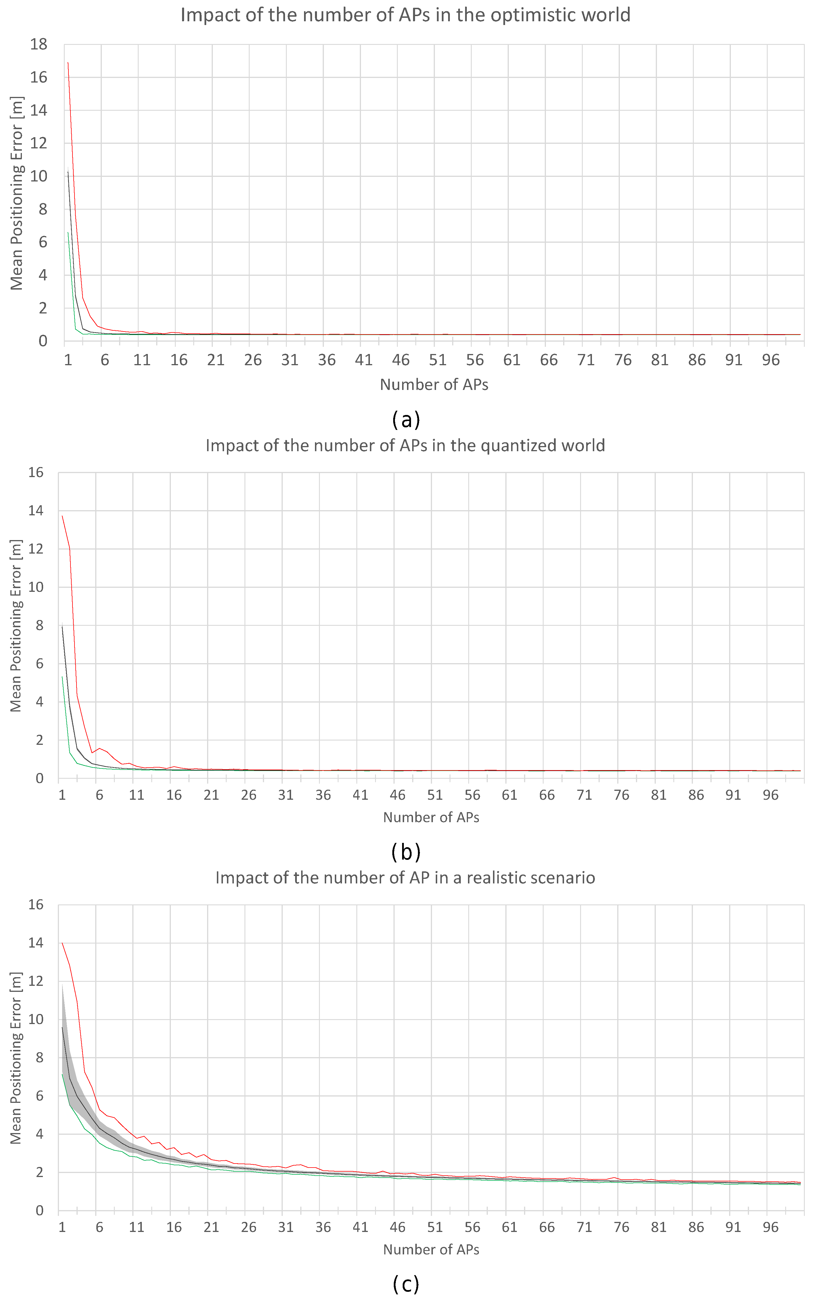
Figure 12.
Impact of the number of APs in the optimistic (a); quantized (b) and realistic noisy (c) worlds. Black lines correspond to the average accuracy over the 100 simulations, green lines correspond to min. accuracy, and the red lines correspond to the max. accuracy.
Figure 12.
Impact of the number of APs in the optimistic (a); quantized (b) and realistic noisy (c) worlds. Black lines correspond to the average accuracy over the 100 simulations, green lines correspond to min. accuracy, and the red lines correspond to the max. accuracy.
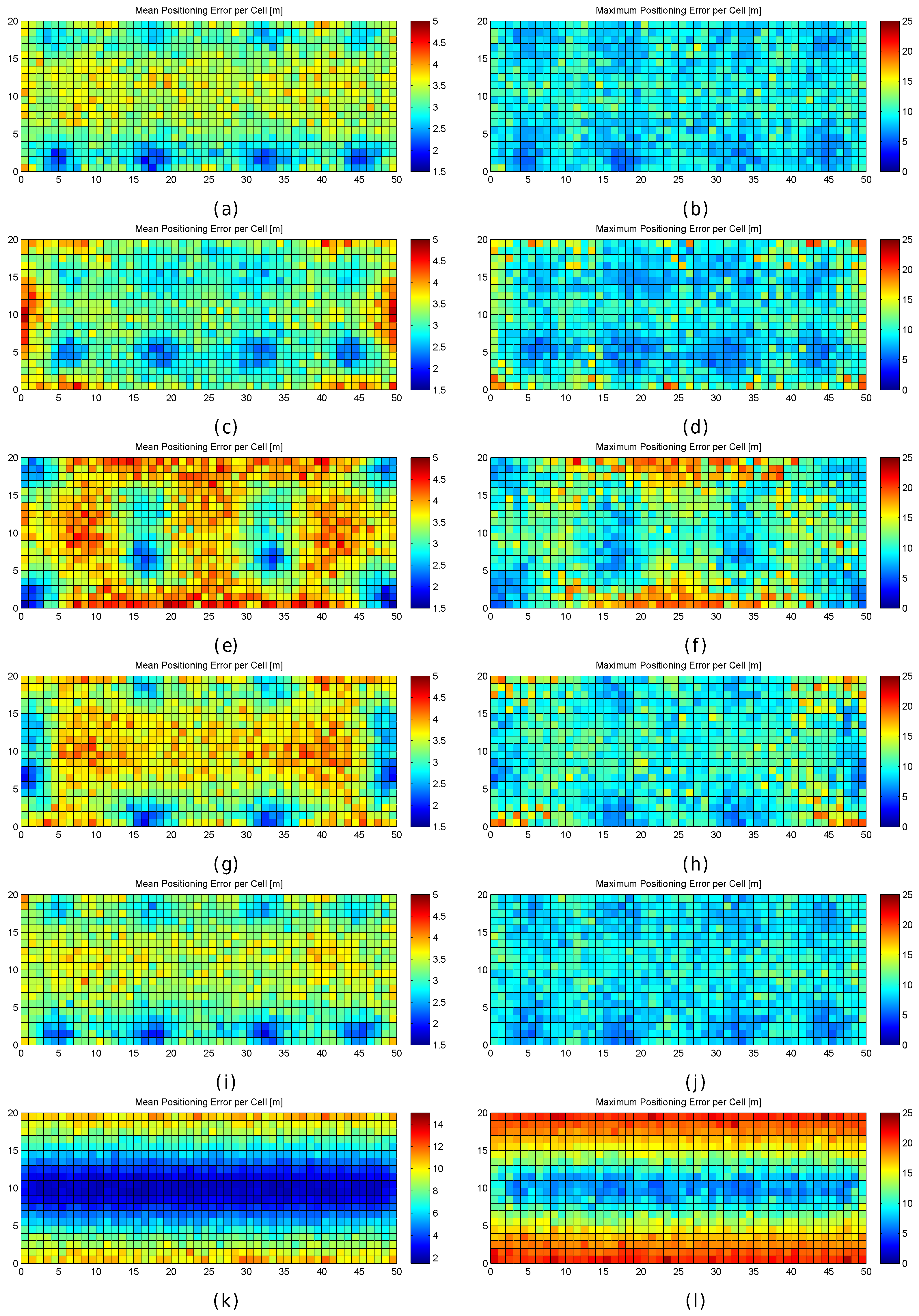
Figure 13.
Graphical results (mean and maximum positioning errors over 100 runs) for analysing the AP distribution in the noisy world. (a,b) original AP distribution; (c,d) alternative AP distribution 1; (e,f) alternative AP distribution 2; (g,h) alternative AP distribution 3; (i,j) alternative AP distribution 4; (k,l) alternative AP distribution 5.
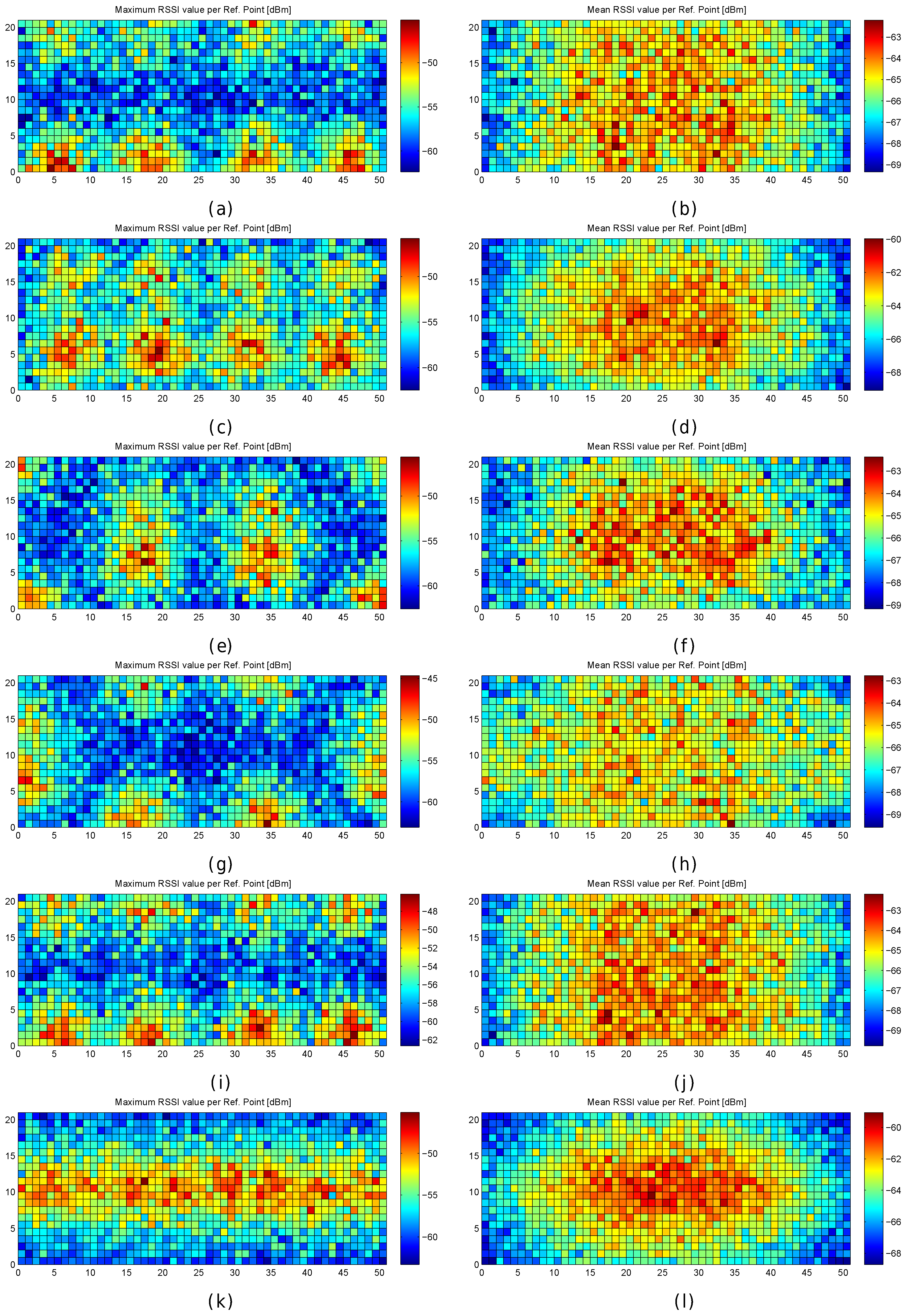
Figure 14.
RSSI Statistics (mean and maximum RSSI value) for analysing the AP distribution in the noisy world (). (a,b) original AP distribution; (c,d) alternative AP distribution 1; (e,f) alternative AP distribution 2; (g,h) alternative AP distribution 3; (i,j) alternative AP distribution 4; (k,l) alternative AP distribution 5.
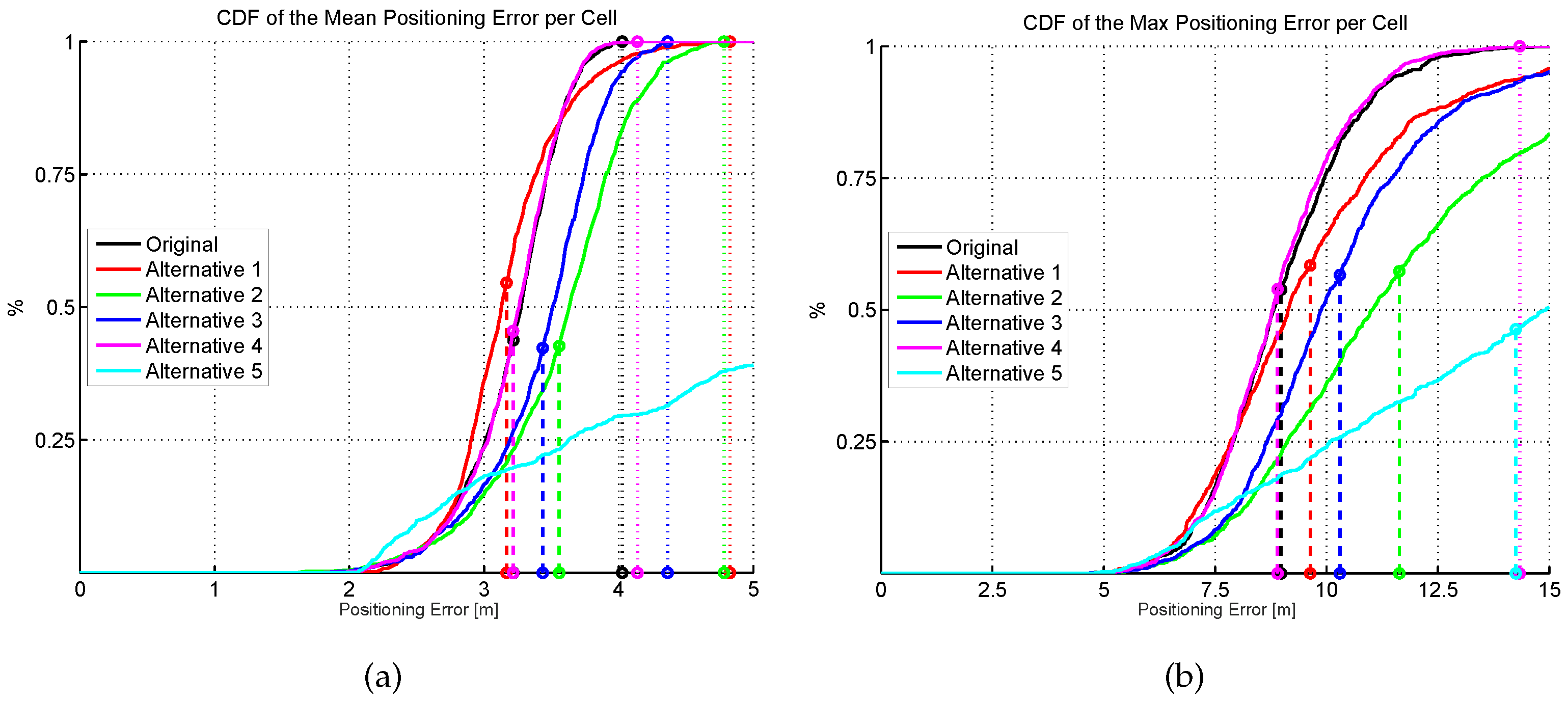
Figure 15.
Cumulative distribution of the mean (a) and maximum (b) positioning error (CDF) for six different AP distributions. Dashed vertical lines indicate the average error, whereas dotted vertical lines indicate the highest error.
Figure 15.
Cumulative distribution of the mean (a) and maximum (b) positioning error (CDF) for six different AP distributions. Dashed vertical lines indicate the average error, whereas dotted vertical lines indicate the highest error.
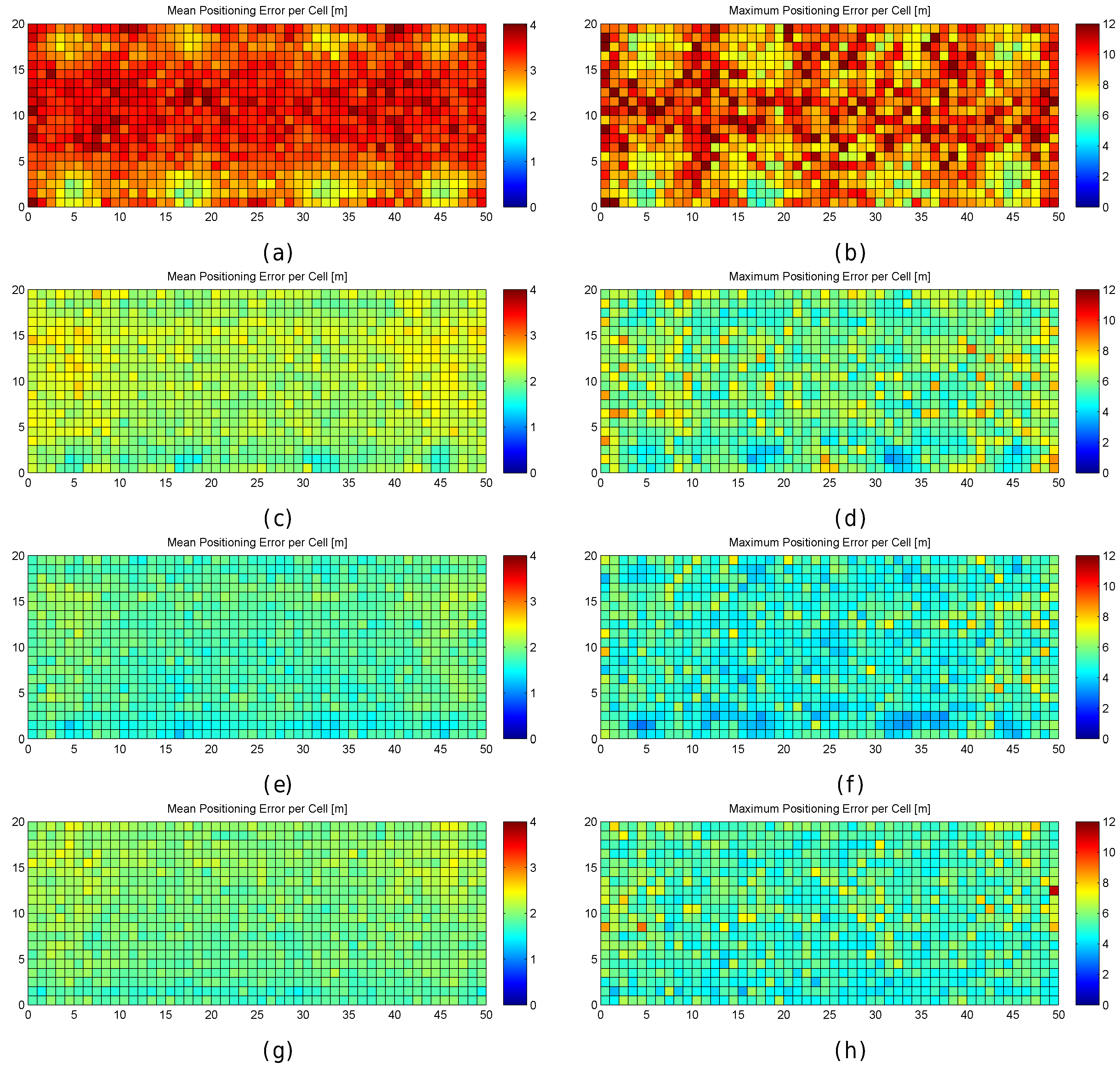
Figure 16.
Graphical results (mean and maximum positioning errors over 100 runs) for analysing virtual APs in the noisy world. (a,b) eight APs, one network per AP; (c,d) eight APs, four networks per AP (concatenated); (e,f) eight APs, four networks per AP (average); (g,h) 32 APs, one network per AP.
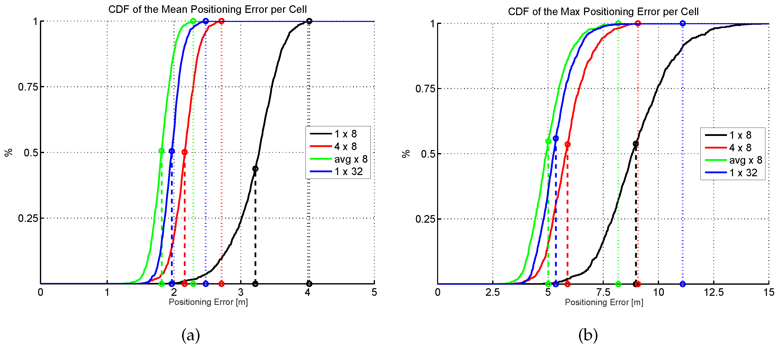
Figure 17.
Cumulative distribution of the mean (a) and max. (b) positioning error (CDF) for comparison of virtual APs. Dashed and dotted vertical lines stand for average and highest error, respectively.
Figure 17.
Cumulative distribution of the mean (a) and max. (b) positioning error (CDF) for comparison of virtual APs. Dashed and dotted vertical lines stand for average and highest error, respectively.
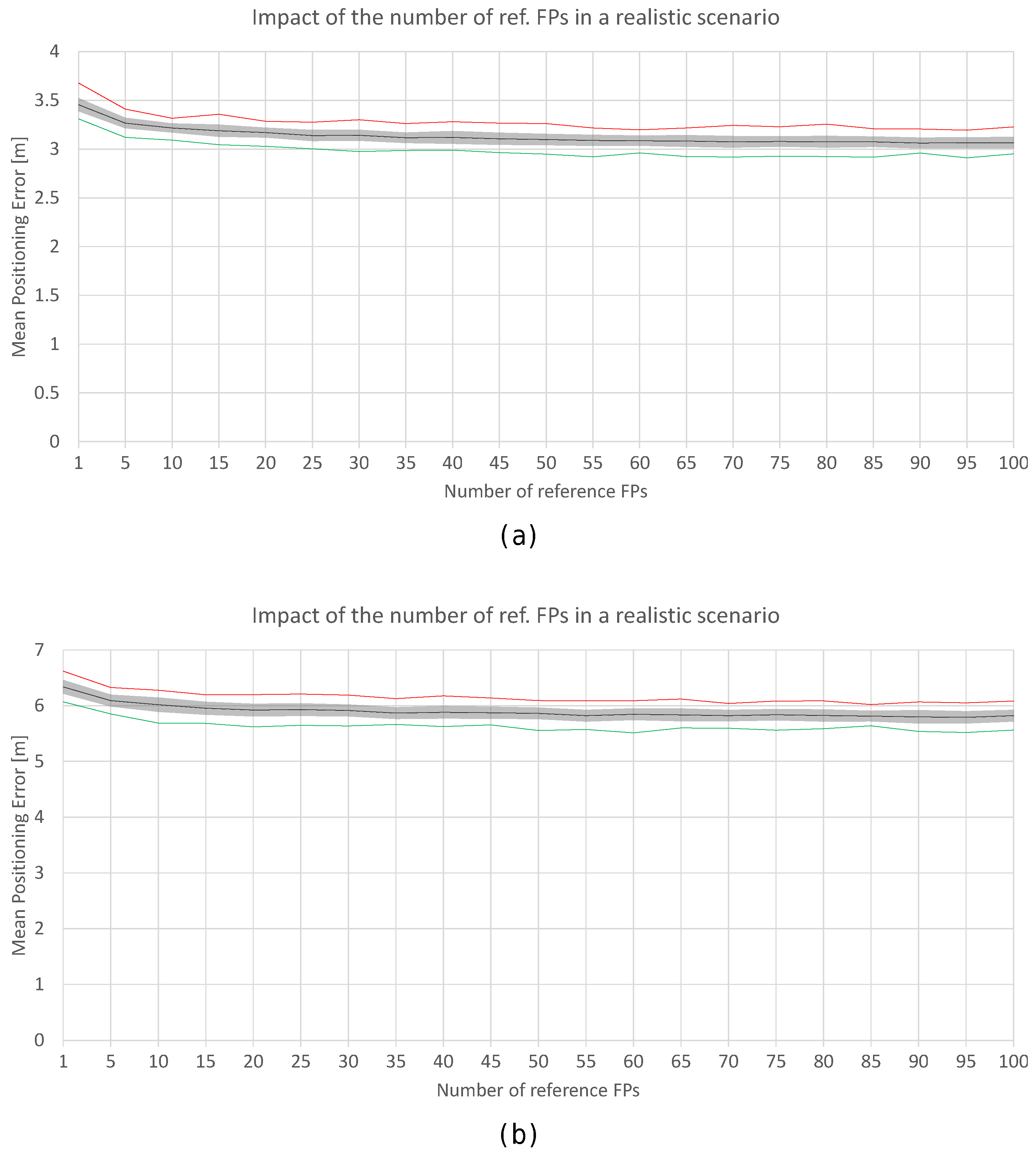
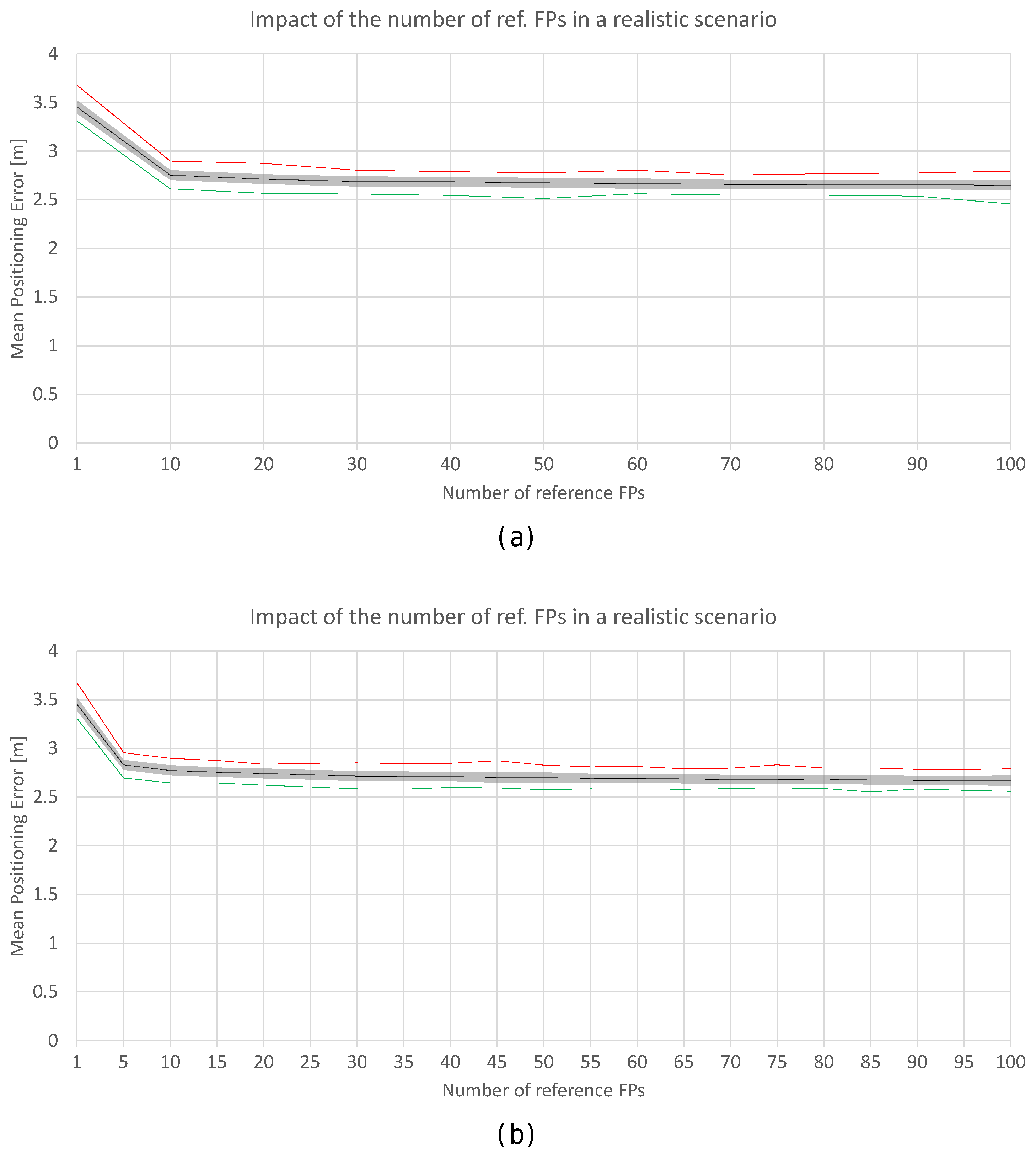
Figure 18.
Impact of the number of reference fingerprints in the realistic world with noise (a) and (b). Black lines correspond to the average accuracy over the 100 simulations, green lines correspond to min. accuracy, and the red lines correspond to the max. accuracy.
Figure 18.
Impact of the number of reference fingerprints in the realistic world with noise (a) and (b). Black lines correspond to the average accuracy over the 100 simulations, green lines correspond to min. accuracy, and the red lines correspond to the max. accuracy.
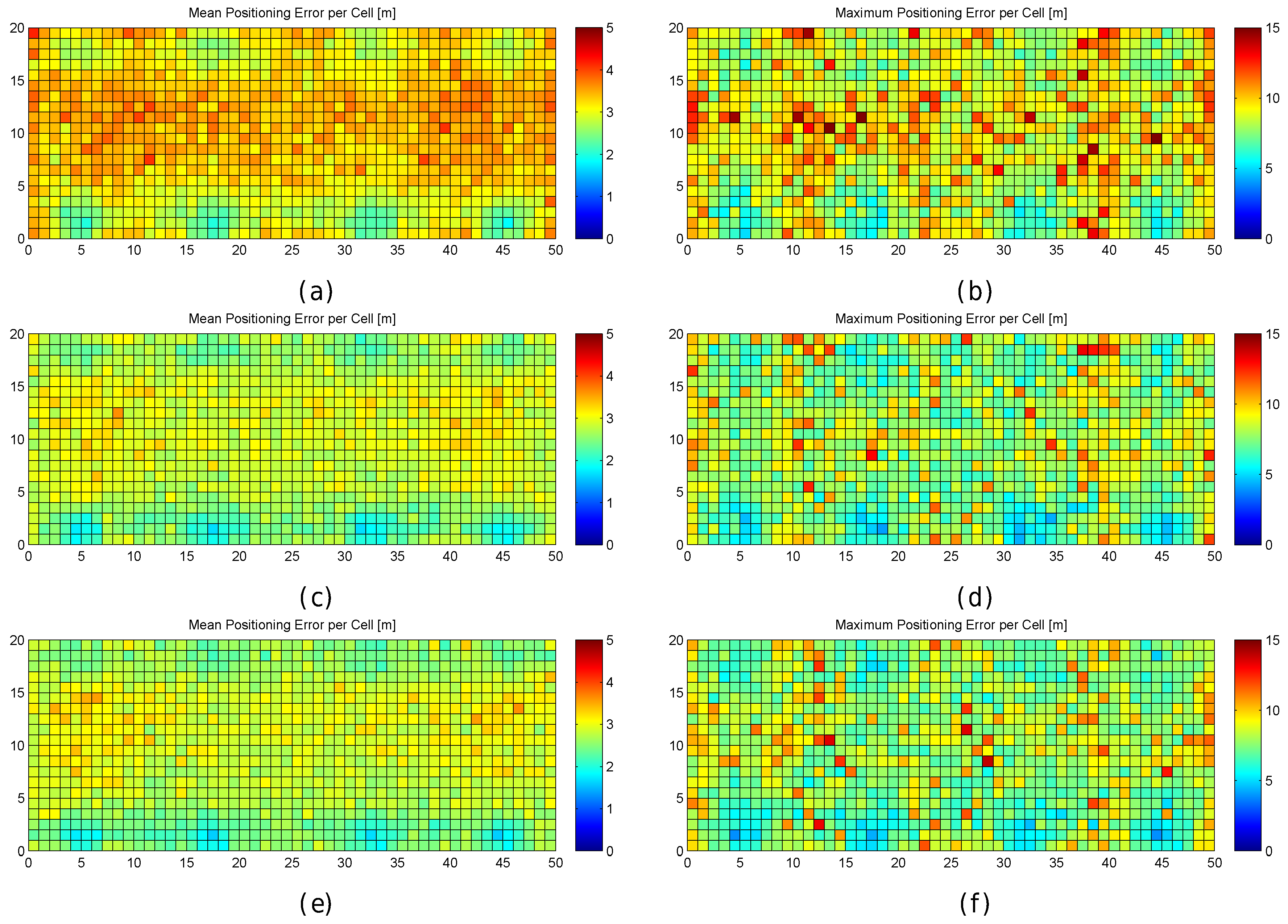
Figure 19.
Graphical results (mean and maximum positioning errors over 100 runs) for analysing the AP distribution in the noisy world. (a,b) one fingerprint per reference point; (c,d) 10 fingerprints per reference point; (e,f) 100 fingerprints per reference point.
Figure 19.
Graphical results (mean and maximum positioning errors over 100 runs) for analysing the AP distribution in the noisy world. (a,b) one fingerprint per reference point; (c,d) 10 fingerprints per reference point; (e,f) 100 fingerprints per reference point.
Figure 20.
Impact of the number of reference fingerprints in the realistic world with averaging in blocks of 5 (a) and averaging in blocks of 10 (b). Black lines correspond to the average accuracy over the 100 simulations; green and red lines correspond to min. and max. accuracy, respectively.
Figure 20.
Impact of the number of reference fingerprints in the realistic world with averaging in blocks of 5 (a) and averaging in blocks of 10 (b). Black lines correspond to the average accuracy over the 100 simulations; green and red lines correspond to min. and max. accuracy, respectively.
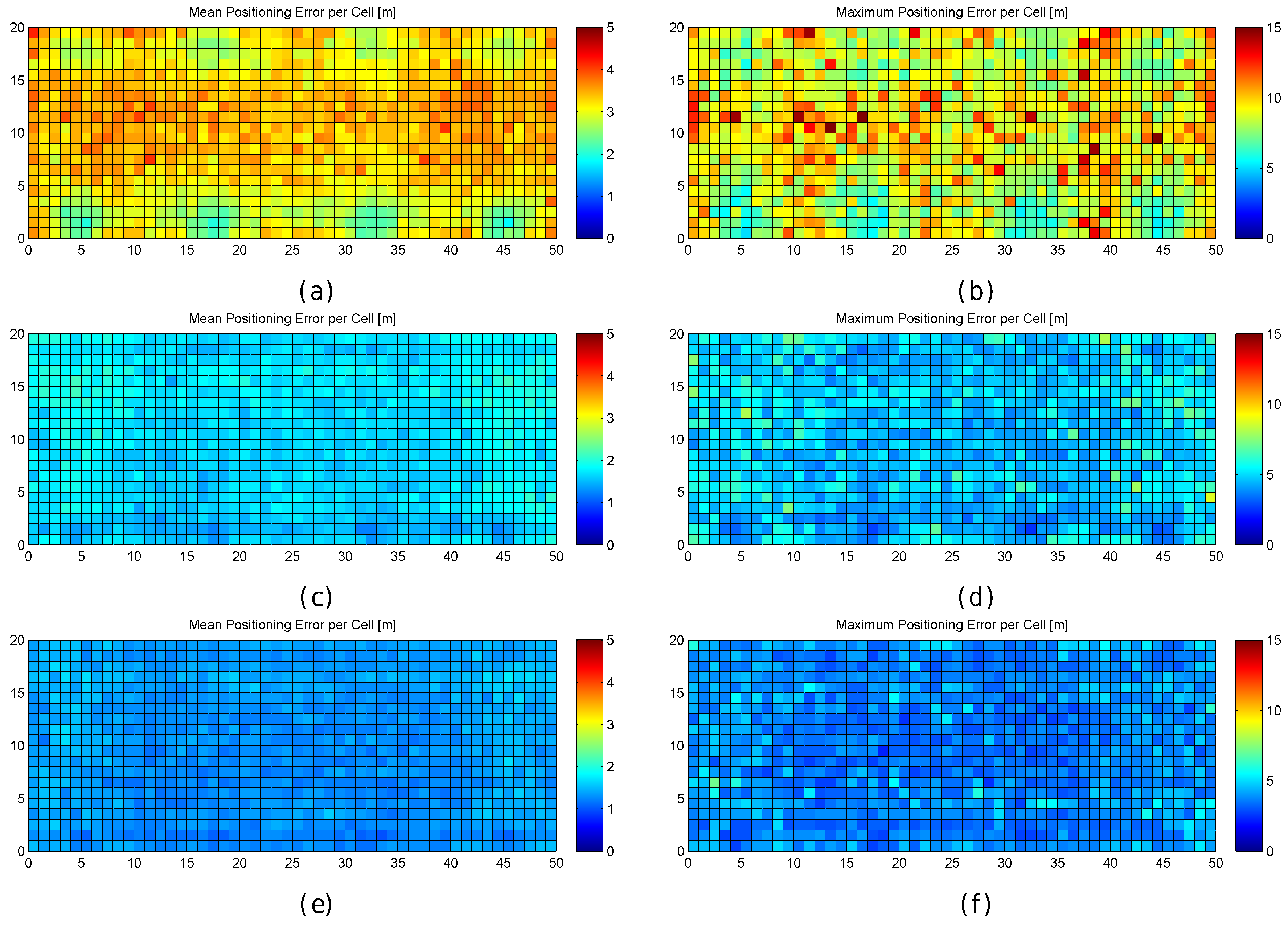
Figure 21.
Graphical results (mean and maximum positioning errors over 100 runs) for analysing the impact of averaging reference fingerprints in the realistic noisy world. (a,b) 10 fingerprints per reference point without averaging; (c,d) 10 fingerprints per reference point with averaging in blocks of 5; (e,f) 10 fingerprints per reference point with averaging in blocks of 10.
Figure 22.
Graphical results (mean and maximum positioning errors over 100 runs) for analysing the impact of averaging training and operational fingerprints in the realistic noisy world. (a,b) 10 fingerprints per reference point without averaging; (c,d) 10 fingerprints per reference point with averaging in blocks of 5; (e,f) 10 fingerprints per reference point with averaging in blocks of 10.
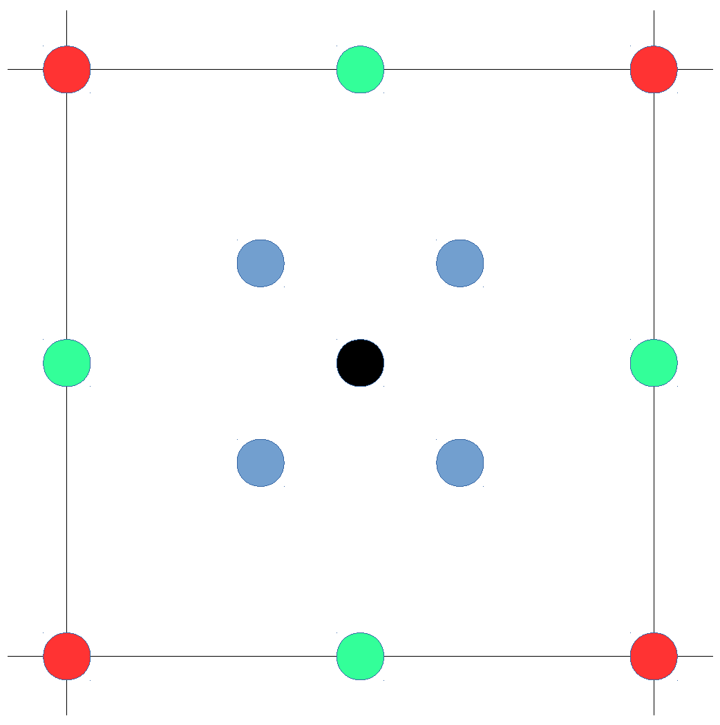
Figure 23.
Expected solutions of kNN in the optimistic world for (red); (green and black); (blue); (black).
Figure 23.
Expected solutions of kNN in the optimistic world for (red); (green and black); (blue); (black).
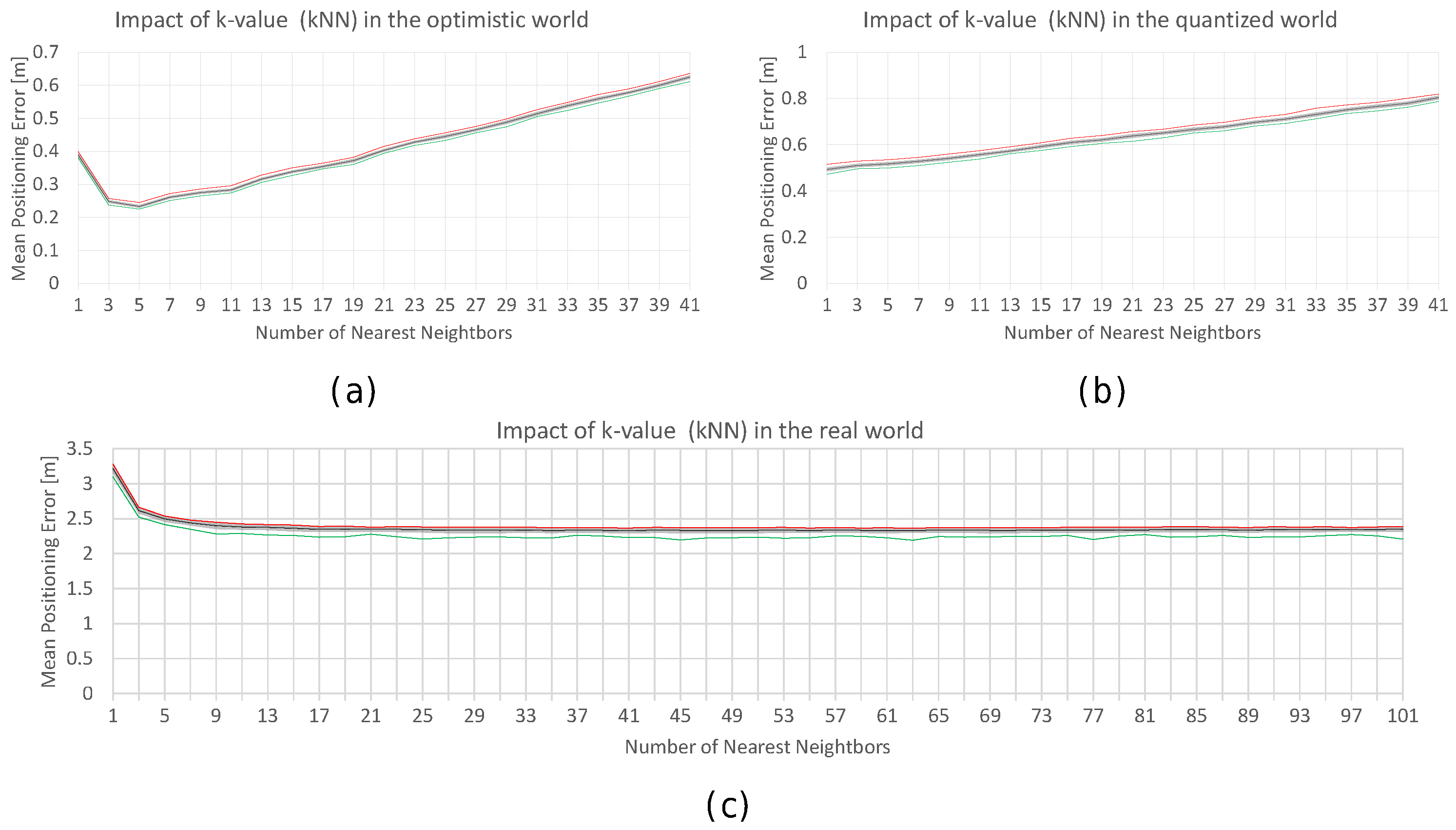
Figure 24.
Impact of the number of reference fingerprints in the optimistic (a); quantized (b) and realistic with (c) worlds. Black, green and red lines correspond to mean, min. and max. accuracy, respectively.
Figure 24.
Impact of the number of reference fingerprints in the optimistic (a); quantized (b) and realistic with (c) worlds. Black, green and red lines correspond to mean, min. and max. accuracy, respectively.
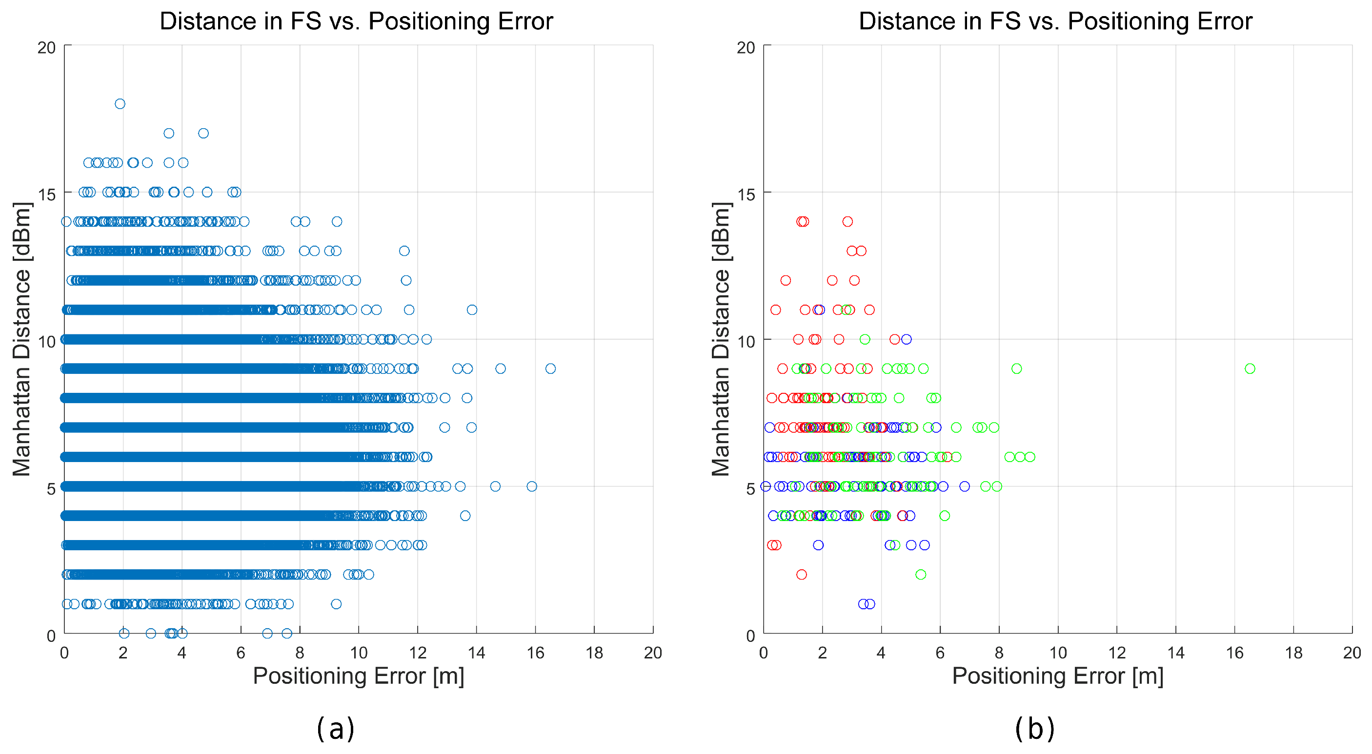
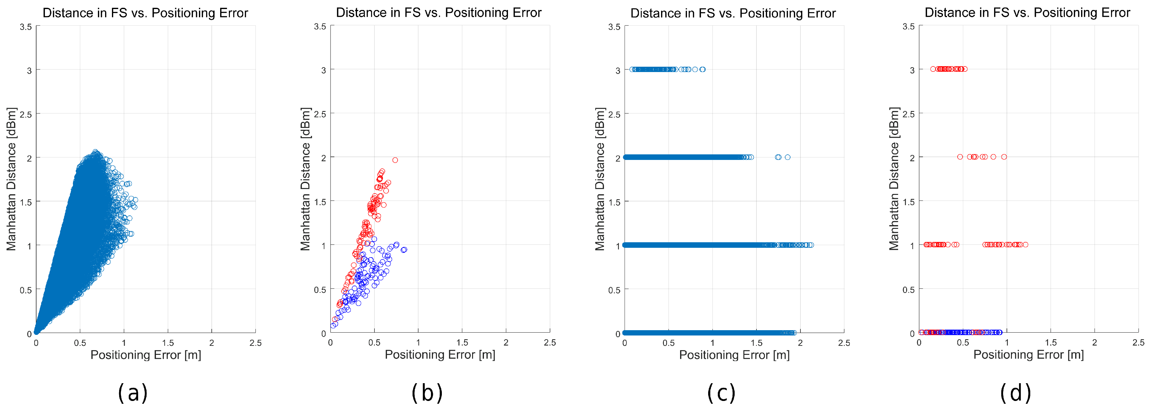
Figure 25.
Relation between the distance in the feature space (Manhattan)—y axis—of the best match and the positioning error—x axis—for the happy world (a,b) and the quantized world (c,d). (a,c) show all the tuples generated in the 100 simulations in all the scenarios; whereas (b) and (d) show the tuples generated in the 100 simulations in two representative cells.
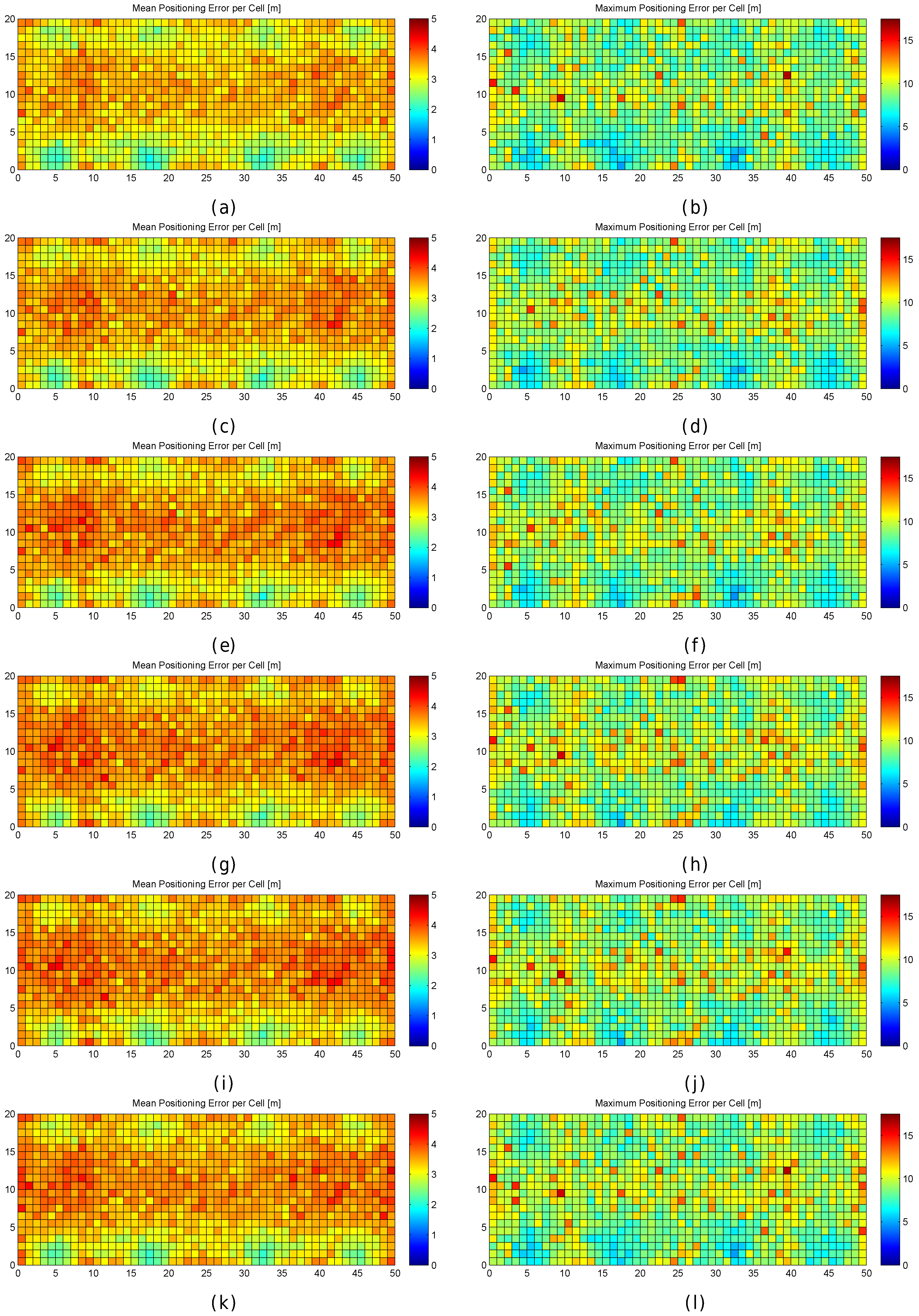
Figure 26.
Graphical results (mean and maximum positioning errors over 100 runs) for analysing the distance/similarity metric in the noisy world for 1-NN. (a,b) Manhattan distance; (c,d) Euclidean distance; (e,f) Mahalanobis distance; (g,h) Matusita distance; (i,j) Neyman distance; (k,l) Sorensen distance.
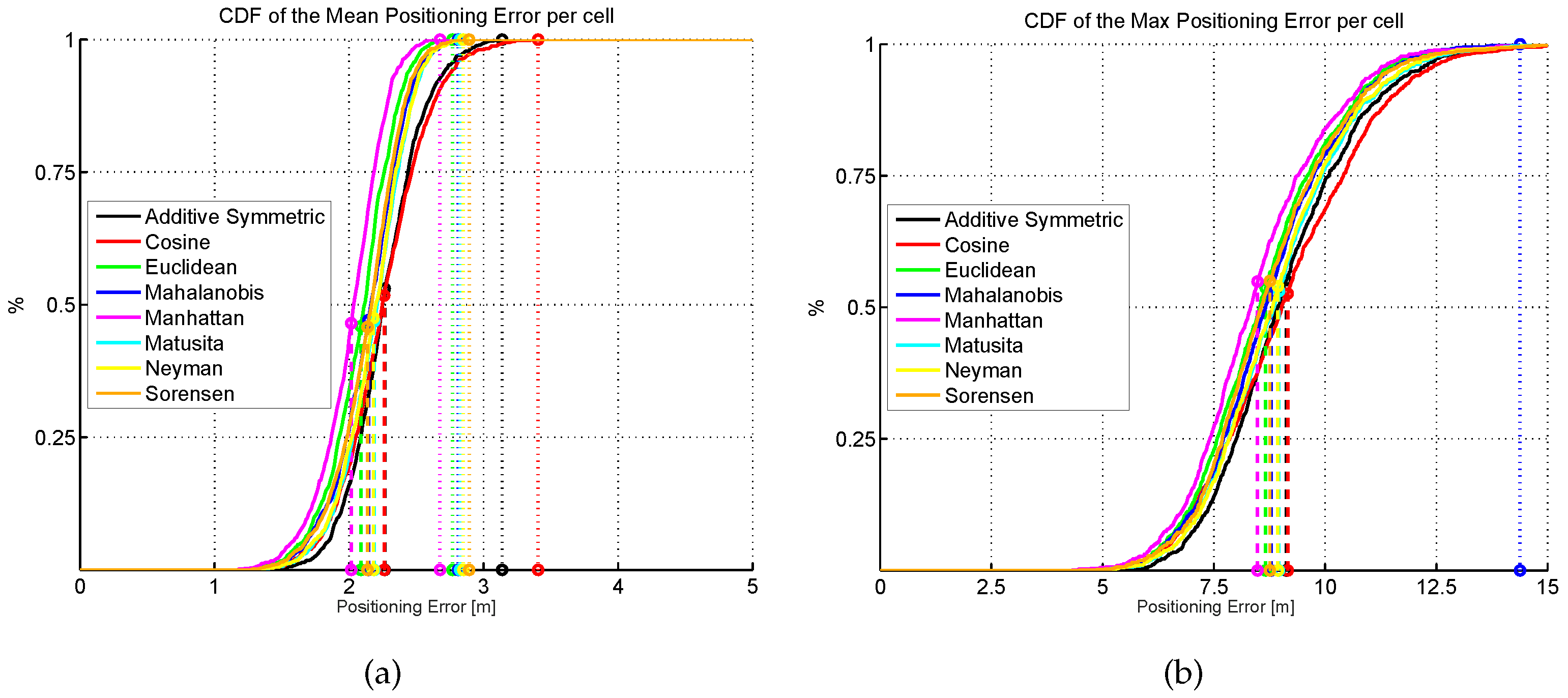
Figure 27.
Cumulative distribution of the mean (a) and maximum (b) positioning error (CDF) for eight different distance/similarity metrics. Dashed vertical lines indicate the average error, whereas dotted vertical lines indicate the highest error.
Figure 27.
Cumulative distribution of the mean (a) and maximum (b) positioning error (CDF) for eight different distance/similarity metrics. Dashed vertical lines indicate the average error, whereas dotted vertical lines indicate the highest error.
Figure 28.
Relation between the distance in the feature space (Manhattan) of the best match and the positioning error for the realistic world. (a) all the tuples generated in the 100 simulations; (b) tuples generated in the 100 simulations in three representative cells.
Figure 28.
Relation between the distance in the feature space (Manhattan) of the best match and the positioning error for the realistic world. (a) all the tuples generated in the 100 simulations; (b) tuples generated in the 100 simulations in three representative cells.
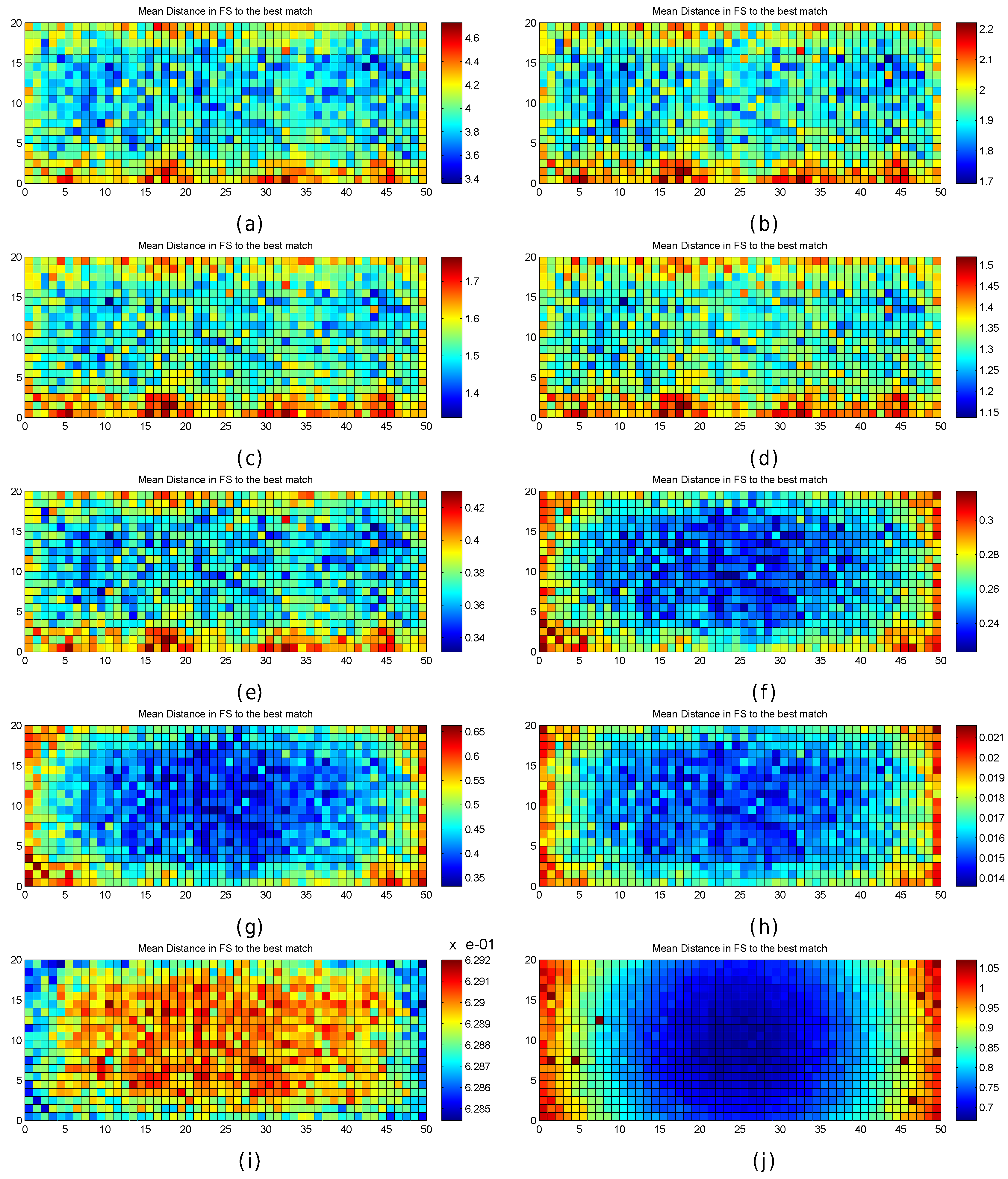
Figure 29.
Mean distance in the feature space to the closest match. (a) Manhattan distance; (b) Euclidean distance; (c) Minkowsky3 distance; (d) Minkowsky5 distance; (e) Mahalanobis distance; (f) Matusita distance; (g) Neyman distance; (h) Sorensen distance; (i) Cosine similarity; (j) Additive Symmetric distance.
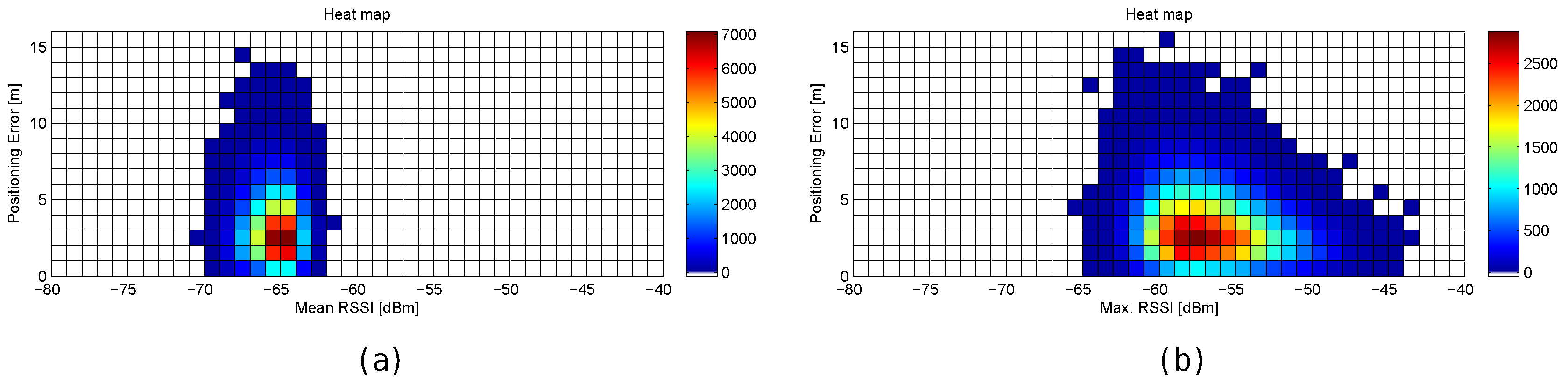
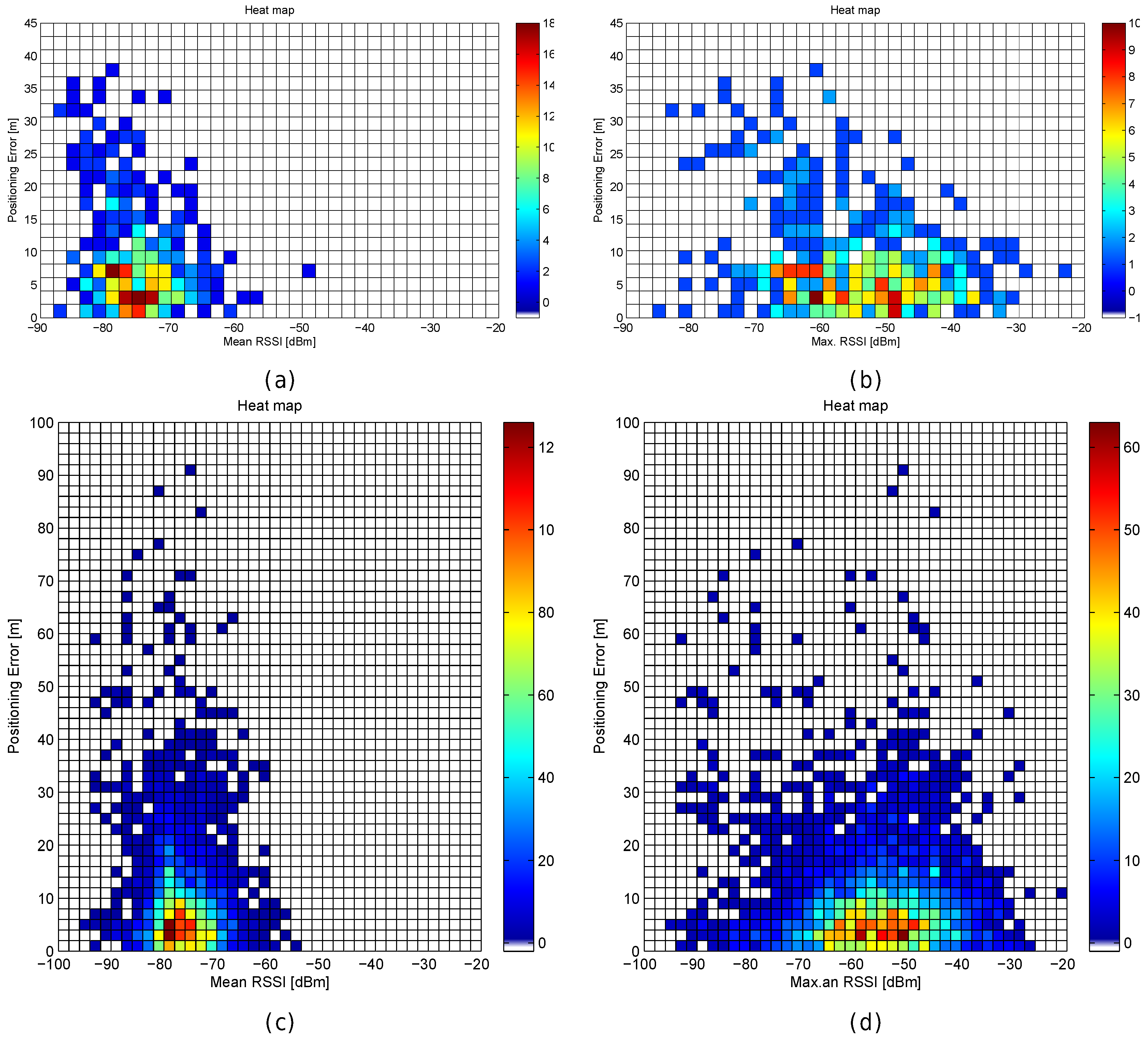
Figure 30.
Relation between positioning error and RSSI statistics (mean RSSI (a) and maximum RSSI value (b)) in the simulated scenario considering the 100 repetitions in the simulation.
Figure 30.
Relation between positioning error and RSSI statistics (mean RSSI (a) and maximum RSSI value (b)) in the simulated scenario considering the 100 repetitions in the simulation.
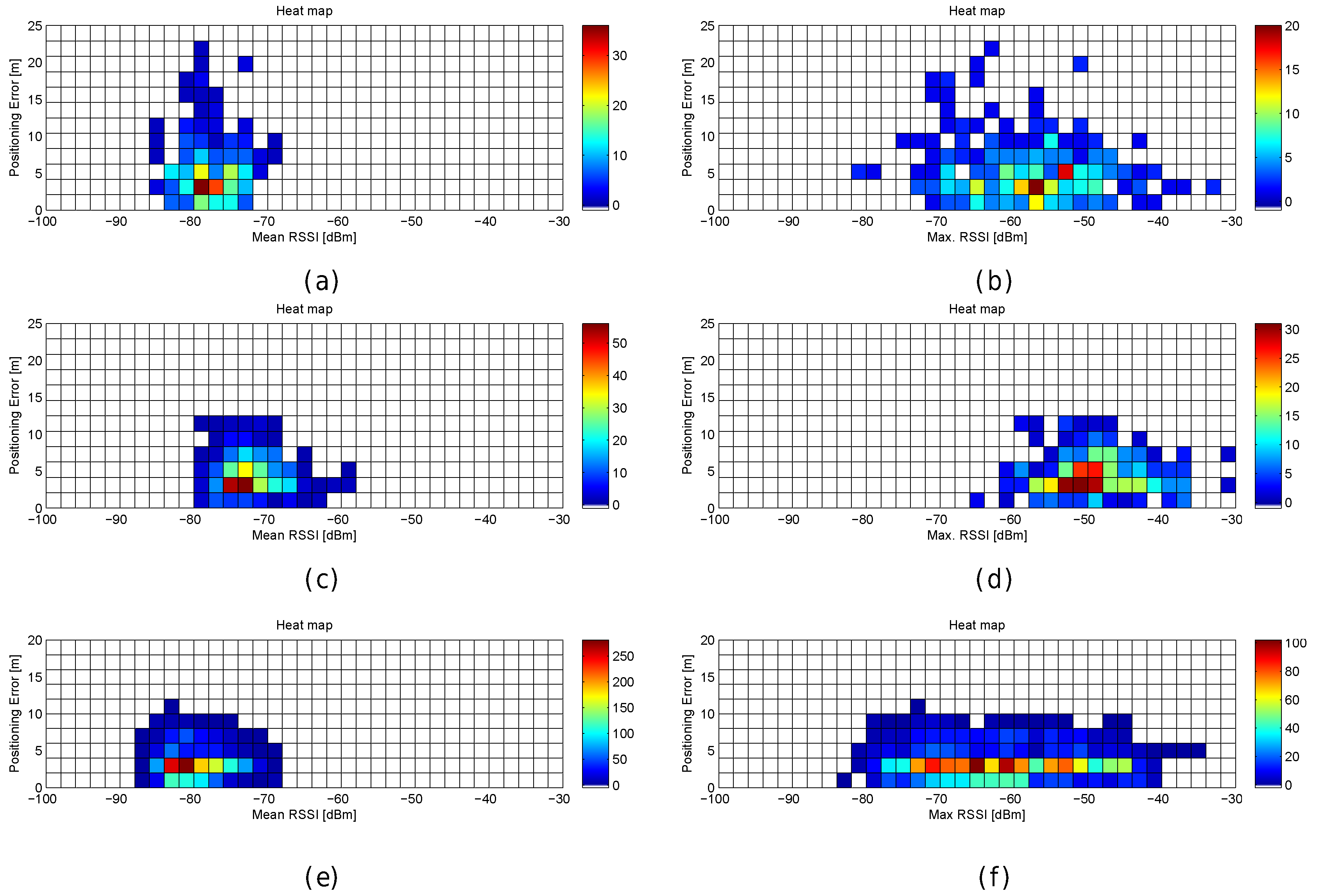
Figure 31.
Relation between positioning error and RSSI statistics (mean RSSI and maximum RSSI value) in real scenarios. (
a,
b) Departamento de Sistemas de Informação, University of Minho; (
c,
d) GEOTEC laboratory, Universitat Jaume I [
53] (
e,
f) Library, Universitat Jaume I [
54].
Figure 31.
Relation between positioning error and RSSI statistics (mean RSSI and maximum RSSI value) in real scenarios. (
a,
b) Departamento de Sistemas de Informação, University of Minho; (
c,
d) GEOTEC laboratory, Universitat Jaume I [
53] (
e,
f) Library, Universitat Jaume I [
54].
Figure 32.
Relation between positioning results in real scenarios and RSSI statistics (mean RSSI and maximum RSSI value). (
a,
b) Technical University of Tampere—Building 1 [
55,
56]; (
c,
d) Technical University of Tampere—Tietolato Building [
57,
58].
Figure 32.
Relation between positioning results in real scenarios and RSSI statistics (mean RSSI and maximum RSSI value). (
a,
b) Technical University of Tampere—Building 1 [
55,
56]; (
c,
d) Technical University of Tampere—Tietolato Building [
57,
58].
Table 1.
Examples of how quantization provides a distance difference of two RSSI with ±1 dBm higher than expected.
Table 1.
Examples of how quantization provides a distance difference of two RSSI with ±1 dBm higher than expected.
| Dist | RSSI | QRSSI | Dist | RSSI | QRSSI | RSSI | QRSSI | Dist [m] | Est. Dist [m] |
|---|
| 1.0593 | −40.50 | −41 | 1.0594 | −40.50 | −41 | ≈0 | 0 | <0.001 | 0 |
| 1.0593 | −40.50 | −41 | 1.0592 | −40.499 | −40 | ≈0 | 1 | <0.001 | ≈0.13 |
| 1.0593 | −40.50 | −41 | 1.1885 | −41.499 | −41 | ≈1 | 0 | ≈0.13 | 0 |
| 1.0593 | −40.50 | −41 | 1.1886 | −41.50 | −42 | ≈1 | 1 | ≈0.13 | ≈0.13 |
| 1.0592 | −40.49 | −40 | 1.1886 | −41.50 | −42 | ≈1 | 2 | ≈0.13 | ≈0.26 |
| 59.5663 | −75.50 | −76 | 59.5664 | −75.5 | −76 | ≈0 | 0 | <1 mm | 0 |
| 59.5663 | −75.50 | −76 | 59.5662 | −75.499 | −75 | ≈0 | 1 | <1 mm | ≈7.27 |
| 59.5663 | −75.50 | −76 | 66.8343 | −76.499 | −76 | ≈1 | 0 | ≈7.27 | 0 |
| 59.5663 | −75.50 | −76 | 66.8344 | −76.50 | −77 | ≈1 | 1 | ≈7.27 | ≈7.27 |
| 59.5662 | −75.49 | −75 | 66.8344 | −76.50 | −77 | ≈1 | 2 | ≈7.27 | ≈14.54 |
| 94.4061 | −79.50 | −80 | 94.4062 | −79.50 | −80 | ≈0 | 0 | <1 mm | 0 m |
| 94.4061 | −79.50 | −80 | 94.4060 | −79.499 | −79 | ≈0 | 1 | <1 mm | ≈11.52 |
| 94.4061 | −79.50 | −80 | 105.9253 | −80.499 | −80 | ≈1 | 0 | ≈11.52 | 0 |
| 94.4061 | −79.50 | −80 | 105.9254 | −80.50 | −81 | ≈1 | 1 | ≈11.52 | ≈11.52 |
| 94.4060 | −79.49 | −79 | 105.9254 | −80.50 | −81 | ≈1 | 2 | ≈11.52 | ≈23.04 |
Table 2.
Analysis of quantization for Wi-Fi fingerprinting using 1-NN.
Table 2.
Analysis of quantization for Wi-Fi fingerprinting using 1-NN.
| | Mean Error | Max. Error | Max. Expected Error | % Cases above the MEE |
|---|
| no quantization | | | | |
| with quantization | | | | |
Table 3.
Analysis of grid size for Wi-Fi fingerprinting in the optimistic world using 1-NN: Mean positioning error; Maximum positioning Error; Maximum expected error (MEE) and percentage of cases above the MEE.
Table 3.
Analysis of grid size for Wi-Fi fingerprinting in the optimistic world using 1-NN: Mean positioning error; Maximum positioning Error; Maximum expected error (MEE) and percentage of cases above the MEE.
| Grid | Mean Error | Max. Error | Max. Expected Error | % Cases above the MEE |
|---|
| 10.0 m | | | | |
| 5.0 m | | | | |
| 2.0 m | | | | |
| 1.0 m | | | | |
| 0.5 m | | | | |
| 0.2 m | | | | |
| 0.1 m | | | | |
Table 4.
Analysis of grid size for Wi-Fi fingerprinting in the quantized world using 1-NN: Mean positioning error; Maximum positioning Error; Maximum expected error (MEE) and percentage of cases above the MEE.
Table 4.
Analysis of grid size for Wi-Fi fingerprinting in the quantized world using 1-NN: Mean positioning error; Maximum positioning Error; Maximum expected error (MEE) and percentage of cases above the MEE.
| Grid | Mean Error | Max. Error | Max. Expected Error | % Cases above the MEE |
|---|
| 10.0 m | | | | |
| 5.0 m | | | | |
| 2.0 m | | | | |
| 1.0 m | | | | |
| 0.5 m | | | | |
| 0.2 m | | | | |
| 0.1 m | | | | |
Table 5.
Analysis of grid size for Wi-Fi fingerprinting in the noisy world using 1-NN: Mean positioning error; Maximum positioning Error; Maximum expected error (MEE) and percentage of cases above MEE.
Table 5.
Analysis of grid size for Wi-Fi fingerprinting in the noisy world using 1-NN: Mean positioning error; Maximum positioning Error; Maximum expected error (MEE) and percentage of cases above MEE.
| Noise | Grid | Mean Error | Max. Error | Max. Expected Error | % Cases above the MEE |
|---|
| 10.0 m | | | | |
| 5.0 m | | | | |
| 2.0 m | | | | |
| 1.0 m | | | | |
| 0.5 m | | | | |
| 10.0 m | | | | |
| 5.0 m | | | | |
| 2.0 m | | | | |
| 1.0 m | | | | |
| 0.5 m | | | | |
| 10.0 m | | | | |
| 5.0 m | | | | |
| 2.0 m | | | | |
| 1.0 m | | | | |
| 0.5 m | | | | |
| 10.0 m | | | | |
| 5.0 m | | | | |
| 2.0 m | | | | |
| 1.0 m | | | | |
| 0.5 m | | | | |
| 10.0 m | | | | |
| 5.0 m | | | | |
| 2.0 m | | | | |
| 1.0 m | | | | |
| 0.5 m | | | | |
Table 6.
Location [x,y,z] of the 8 APs.
Table 6.
Location [x,y,z] of the 8 APs.
| AP Distribution | AP 1/AP 5 | AP 2/AP 6 | AP 3/AP 7 | AP 4/AP 8 |
|---|
| Configuration 1 | [625,500,390] | [1875,500,390] | [3150,500,390] | [4375,500,390] |
| [625,1500,540] | [1875,1500,540] | [3150,1500,540] | [4375,1500,540] |
| Configuration 2 | [0,0,390] | [1666,666,390] | [3333,666,390] | [5000,0,390] |
| [000,2000,540] | [1666,1333,540] | [3333,1333,540] | [5000,2000,540] |
| Configuration 3 | [000,666,390] | [1666,0,390] | [3333,0,390] | [5000,666,390] |
| [000,1333,540] | [1666,2000,540] | [3333,2000,540] | [5000,1333,540] |
| Configuration 4 | [500,100,390] | [1750,100,390] | [3250,100,390] | [4500,100,390] |
| [500,1900,540] | [1750,1900,540] | [3250,1900,540] | [4500,1900,540] |
| Configuration 5 | [313,1000,390] | [938,1000,390] | [1563,1000,390] | [2188,1000,390] |
| [2813,1000,390] | [3438,1000,390] | [4063,1000,390] | [4688,1000,390] |
Table 7.
Analysis of AP distribution for Wi-Fi fingerprinting using 1-NN.
Table 7.
Analysis of AP distribution for Wi-Fi fingerprinting using 1-NN.
| AP Dist | Mean Error | Max. Error | Max. Expected Error | % Cases above the MEE |
|---|
| Orig | | | | |
| Alt 1 | | | | |
| Alt 2 | | | | |
| Alt 3 | | | | |
| Alt 4 | | | | |
| Alt 5 | | | | |
Table 8.
Analysis of virtual APs for Wi-Fi fingerprinting in the realistic world using 1-NN.
Table 8.
Analysis of virtual APs for Wi-Fi fingerprinting in the realistic world using 1-NN.
| AP Dist | Independent | Mean Error | Max. Error | Max. Expected Error | % Cases above the MEE |
|---|
| 1 × 8 AP | - | | | | |
| 1 × 32 AP | - | | | | |
| 4 × 8 AP | yes | | | | |
| avg × 8 AP | yes | | | | |
| 4 × 8 AP | partial | | | | |
| avg × 8 AP | partial | | | | |
| 4 × 8 AP | no | | | | |
| avg × 8 AP | no | | | | |
Table 9.
Analysis of averaging training and operational fingerprints in the noisy world using 1-NN.
Table 9.
Analysis of averaging training and operational fingerprints in the noisy world using 1-NN.
| # Ref. FP | Ref. avg. | Op. avg. | Mean Error | Max. Error | MEE | % Cases above the MEE |
|---|
| 1 | no avg | no avg | | | | |
| 10 | no avg | no avg | | | | |
| 10 | no avg | 5 | | | | |
| 10 | no avg | 10 | | | | |
| 10 | 5 | no avg | | | | |
| 10 | 5 | 5 | | | | |
| 10 | 10 | no avg | | | | |
| 10 | 10 | 10 | | | | |
| 100 | 5 | 5 | | | | |
| 100 | 10 | 10 | | | | |
Table 10.
Analysis of the k-Value for Wi-Fi fingerprinting in the noisy world using k-NN: Mean positioning error; Maximum positioning Error; Maximum expected error (MEE) and percentage of cases above the MEE.
Table 10.
Analysis of the k-Value for Wi-Fi fingerprinting in the noisy world using k-NN: Mean positioning error; Maximum positioning Error; Maximum expected error (MEE) and percentage of cases above the MEE.
| k-Value | Mean Error | Max. Error | Max. Expected Error | % Cases above the MEE |
|---|
| 1 | | | | |
| 3 | | | | |
| 5 | | | | |
| 7 | | | | |
| 9 | | | | |
| 11 | | | | |
| 13 | | | | |
| 15 | | | | |
| 17 | | | | |
| 19 | | | | |
| 21 | | | | |
| 23 | | | | |
| 25 | | | | |
| 27 | | | | |
| 29 | | | | |
| 31 | | | | |
| 33 | | | | |
| 35 | | | | |
| 37 | | | | |
| 39 | | | | |
| 41 | | | | |
| 43 | | | | |
| 45 | | | | |
| 47 | | | | |
| 49 | | | | |
| 51 | | | | |
| 53 | | | | |
| 55 | | | | |
| 57 | | | | |
| 59 | | | | |
| 61 | | | | |
| 63 | | | | |
| 65 | | | | |
| 67 | | | | |
| 69 | | | | |
| 71 | | | | |
| 73 | | | | |
| 75 | | | | |
Table 11.
Analysis of similarity/distance metrics for Wi-Fi fingerprinting in the optimistic and quantized worlds using 1-NN.
Table 11.
Analysis of similarity/distance metrics for Wi-Fi fingerprinting in the optimistic and quantized worlds using 1-NN.
| Metric | Optimistic | Quantized |
|---|
| MeanPE | MaxPE | % | Corr. | MeanPE | MaxPE | % | Corr. |
|---|
| additivesymmetric | | | | | | | | |
| bhattacharyya | | | | | | | | |
| camberra | | | | | | | | |
| chebyshev | | | | | | | | |
| cityblock | | | | | | | | |
| cityblockintersect | | | | | | | | |
| clarck | | | | | | | | |
| cosine | | | | | | | | |
| divergence | | | | | | | | |
| euclidean | | | | | | | | |
| fidelity | | | | | | | | |
| harmonicmean | | | | | | | | |
| hellinger | | | | | | | | |
| innerproduct | | | | | | | | |
| jeffreys | | | | | | | | |
| jensen-difference | | | | | | | | |
| jensen-shannon | | | | | | | | |
| k-divergence | | | | | | | | |
| kullback-leibler | | | | | | | | |
| kumar-hassebrook | | | | | | | | |
| KumarJohnson | | | | | | | | |
| lorentzian | | | | | | | | |
| mahalanobis | | | | | | | | |
| matusita | | | | | | | | |
| MaxSymetricChi2 | | | | | | | | |
| minkowsky3 | | | | | | | | |
| minkowsky4 | | | | | | | | |
| minkowsky5 | | | | | | | | |
| MinSymetricChi2 | | | | | | | | |
| motyka | | | | | | | | |
| neyman | | | | | | | | |
| pearson | | | | | | | | |
| sorensen | | | | | | | | |
| squared | | | | | | | | |
| squaredchord | | | | | | | | |
| Taneja | | | | | | | | |
| topsoe | | | | | | | | |
| VicisSymetricChi2A | | | | | | | | |
| VicisSymetricChi2B | | | | | | | | |
| VicisSymetricChi2C | | | | | | | | |
| VicisWaveHedges | | | | | | | | |
| wavehedges | | | | | | | | |
Table 12.
Analysis of similarity/distance metrics for Wi-Fi fingerprinting in the realistic world using 1-NN.
Table 12.
Analysis of similarity/distance metrics for Wi-Fi fingerprinting in the realistic world using 1-NN.
| Metric | Optimistic |
|---|
| MeanPE | MaxPE | % | Corr. |
|---|
| additivesymmetric | | | | |
| cityblock | | | | |
| cosine | | | | |
| euclidean | | | | |
| mahalanobis | | | | |
| matusita | | | | |
| minkowsky3 | | | | |
| minkowsky4 | | | | |
| minkowsky5 | | | | |
| neyman | | | | |
| sorensen | | | | |


