Magnetic Flux Distribution of Linear Machines with Novel Three-Dimensional Hybrid Magnet Arrays

Abstract
:1. Introduction
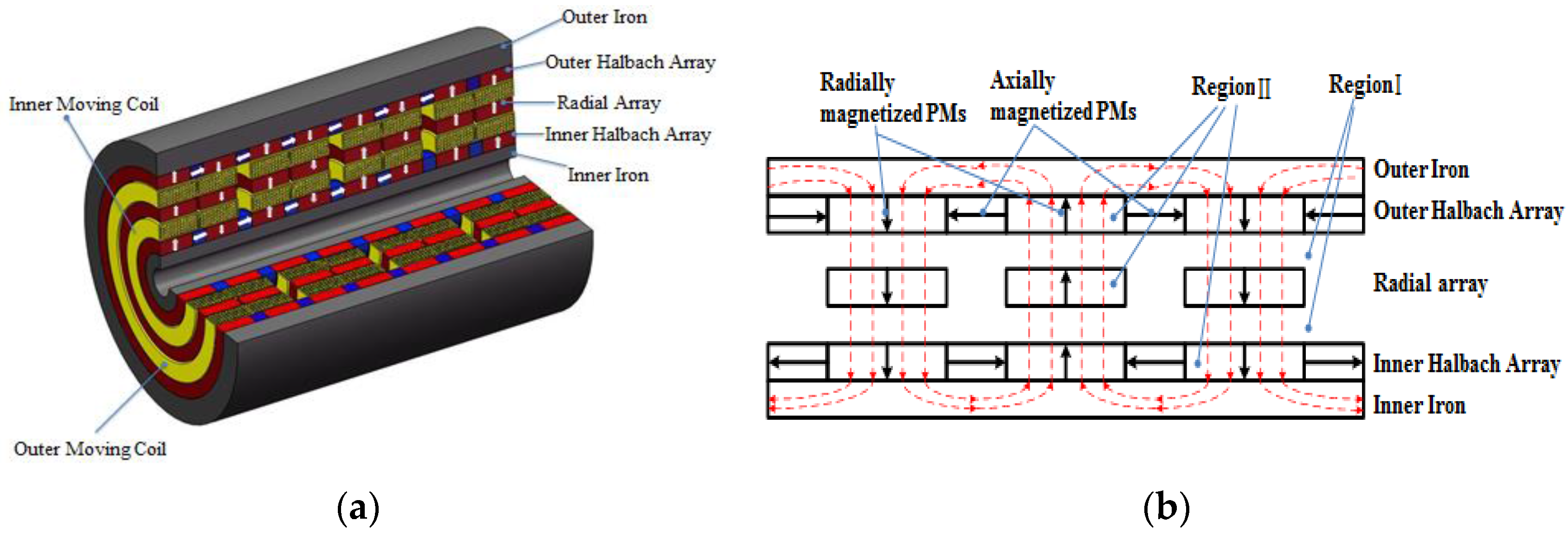
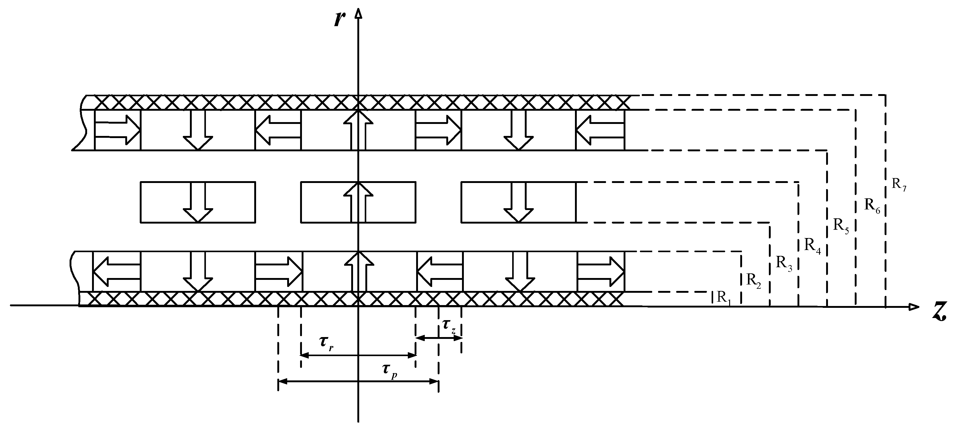
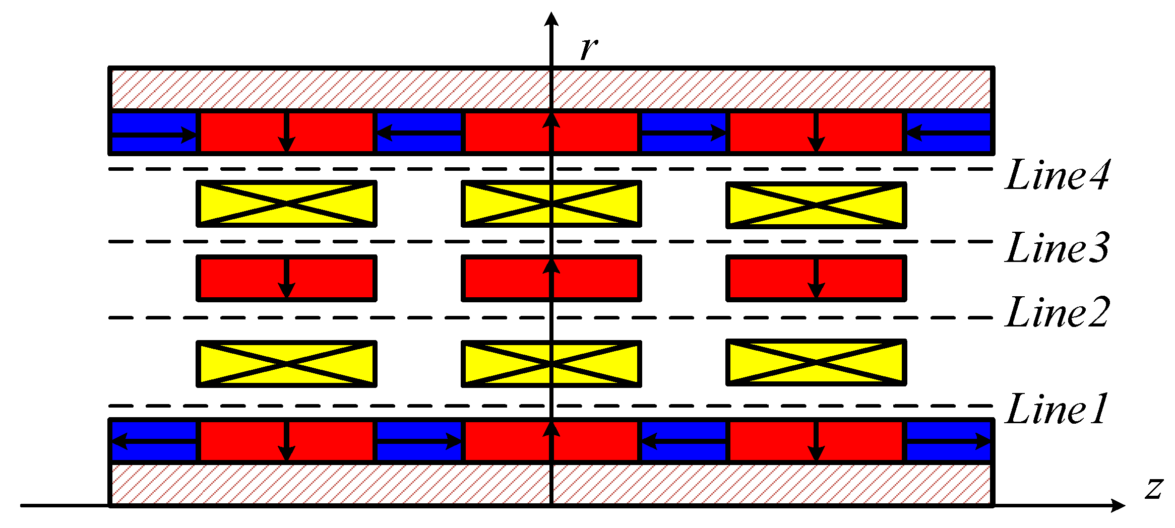
2. Concept Design
3. Governing Equations
3.1. Assumptions
- (a)
- The machine has a periodic magnetic structure along axial direction z.
- (b)
- The axial length is infinite, and thus the end effects can be ignored.
- (c)
- The distribution of magnetic field is axially symmetric.
- (d)
- The magnetic permeability of back iron is infinite.
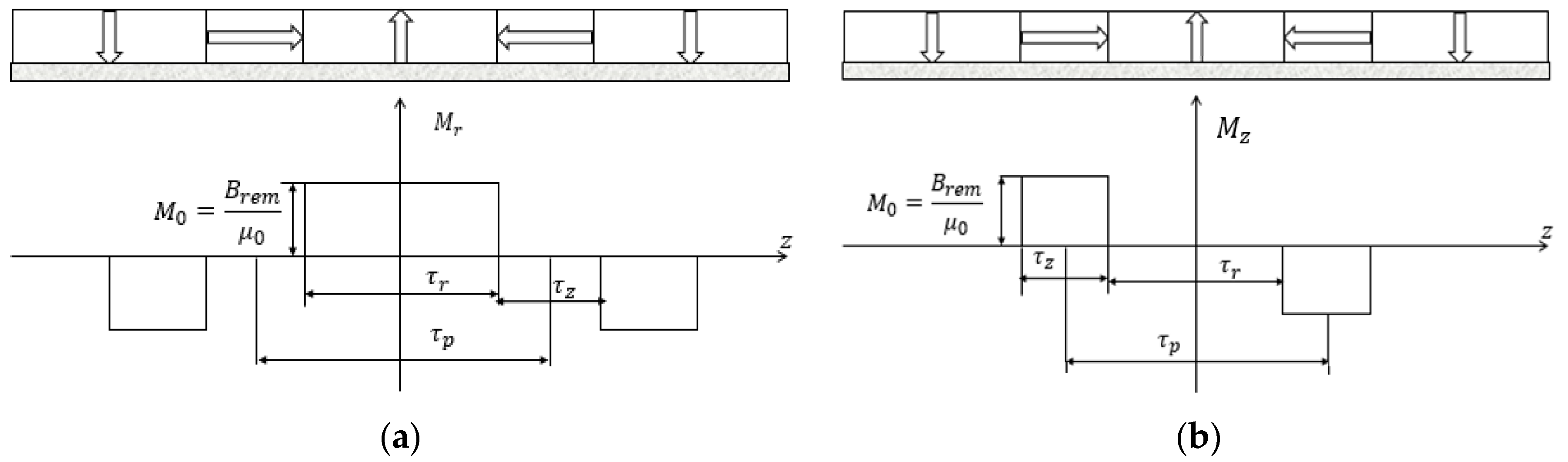
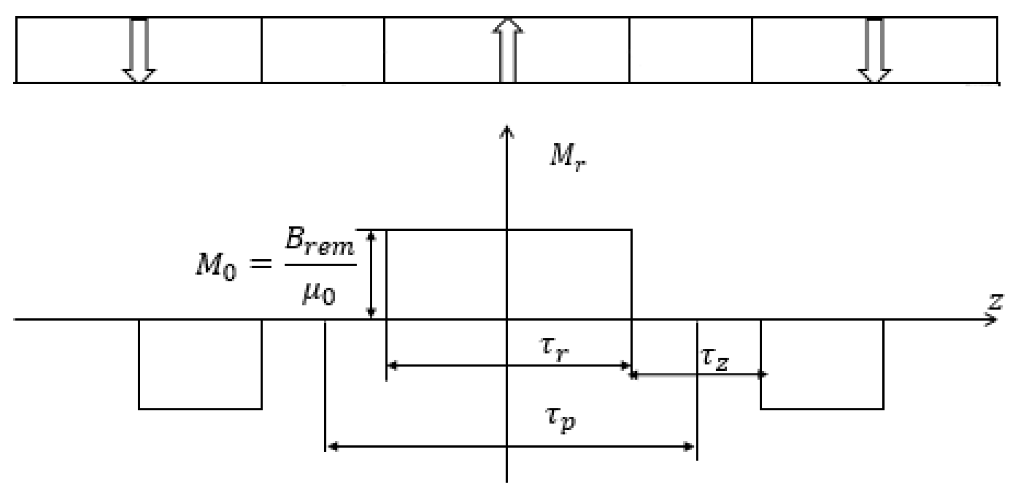
3.2. Characterization of Materials and Governing Equations
4. Formulation of Magnetic Field
4.1. General Solution to Magnetic Potential in Region I
4.2. General Solution to Magnetic Potential in Region II
4.3. Analytical Model of Flux Density
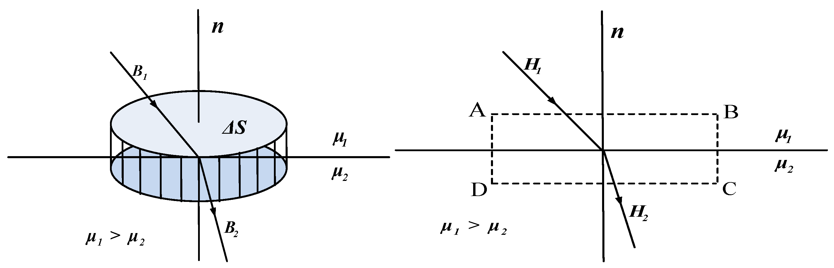
4.4. Boundary Conditions
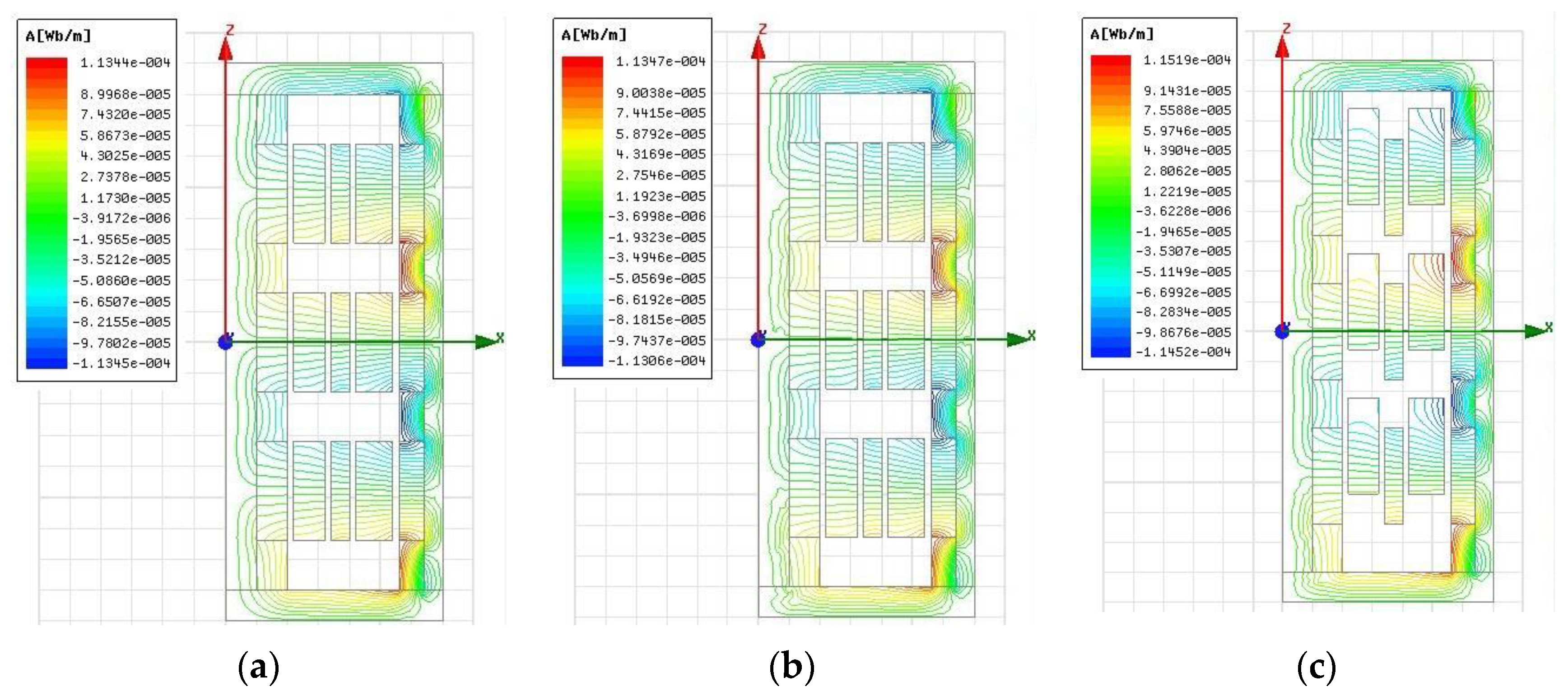
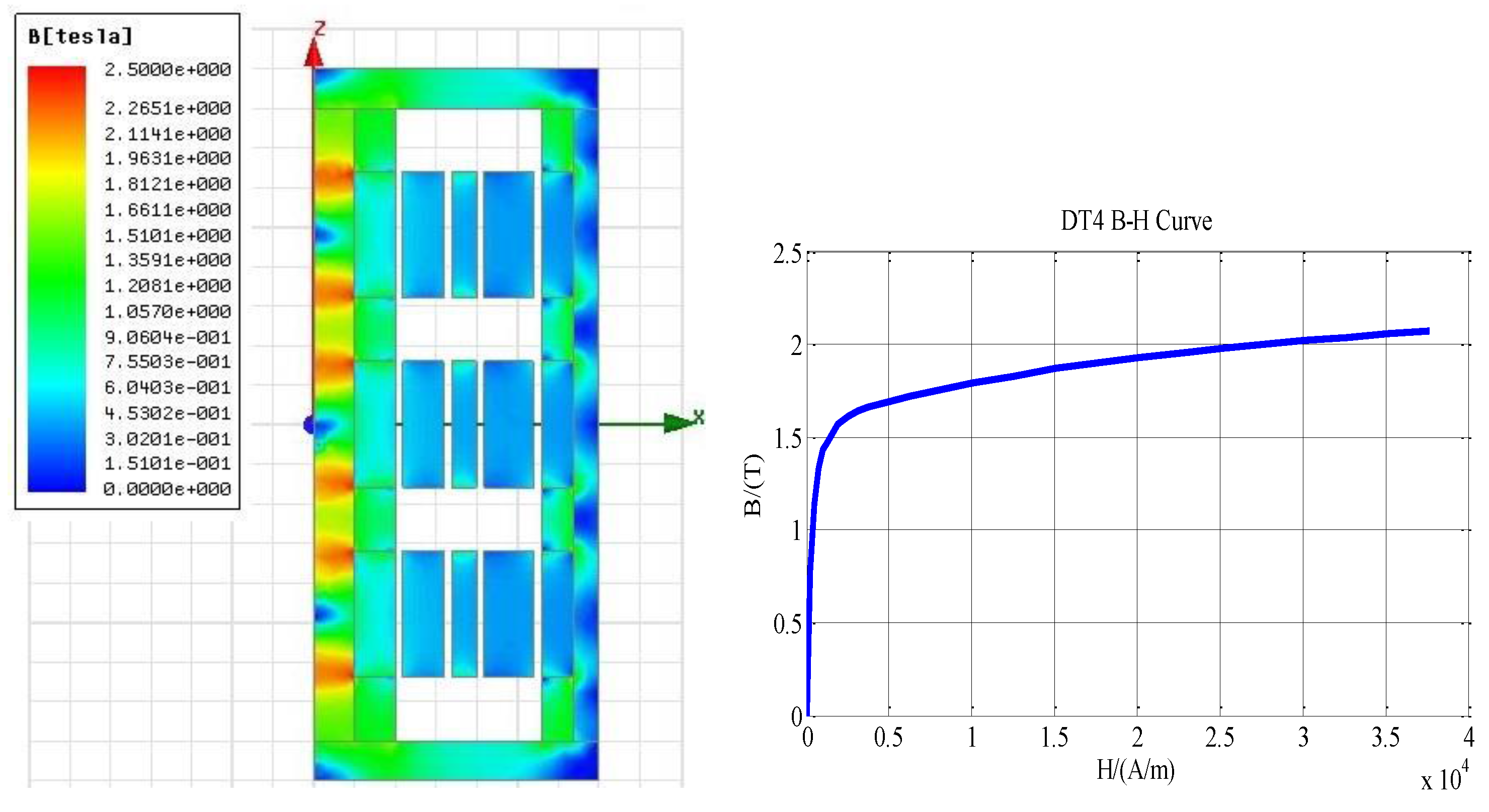
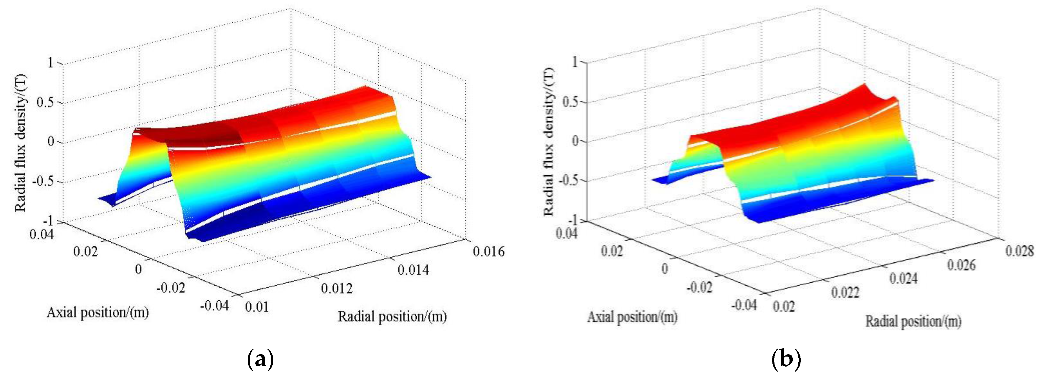
5. Numerical Simulation and Analysis
5.1. Numerical Model
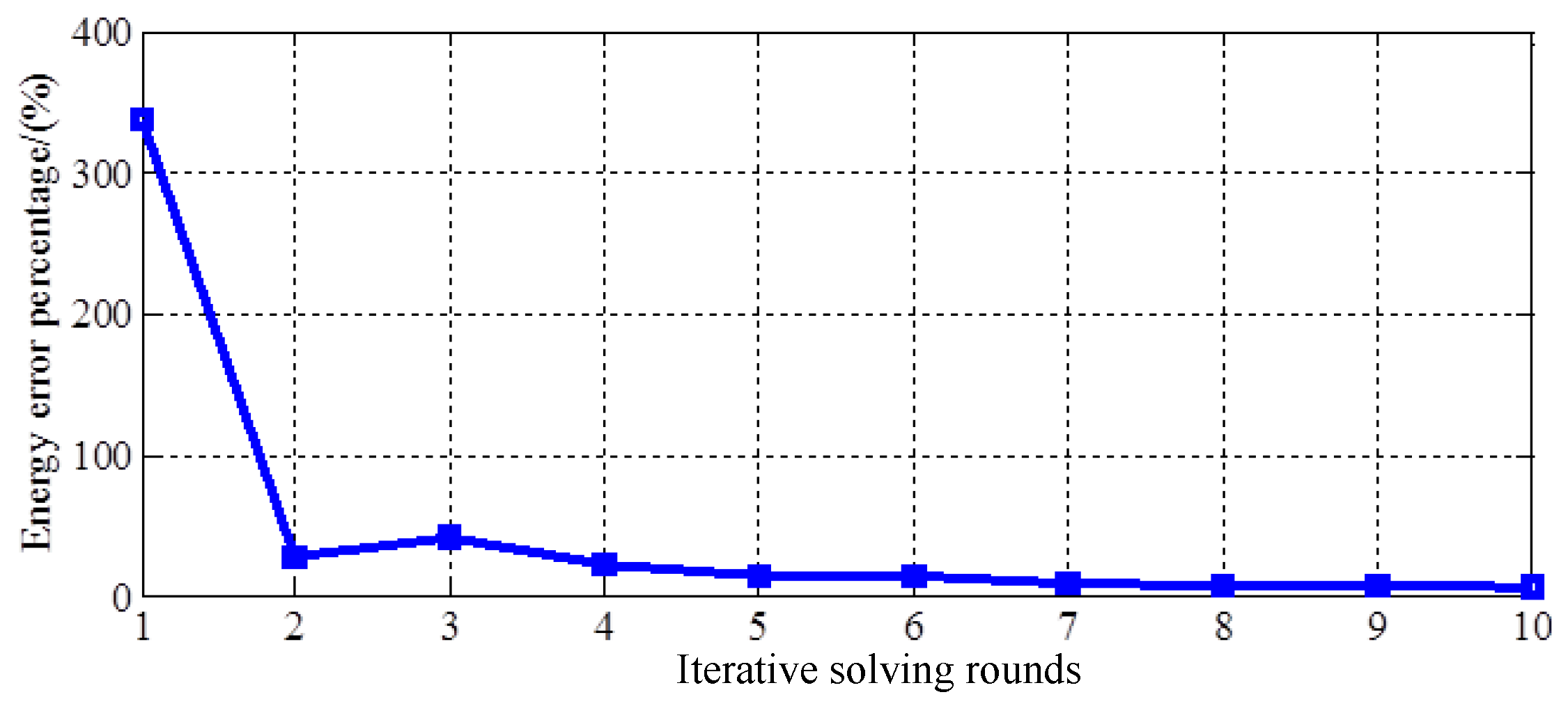
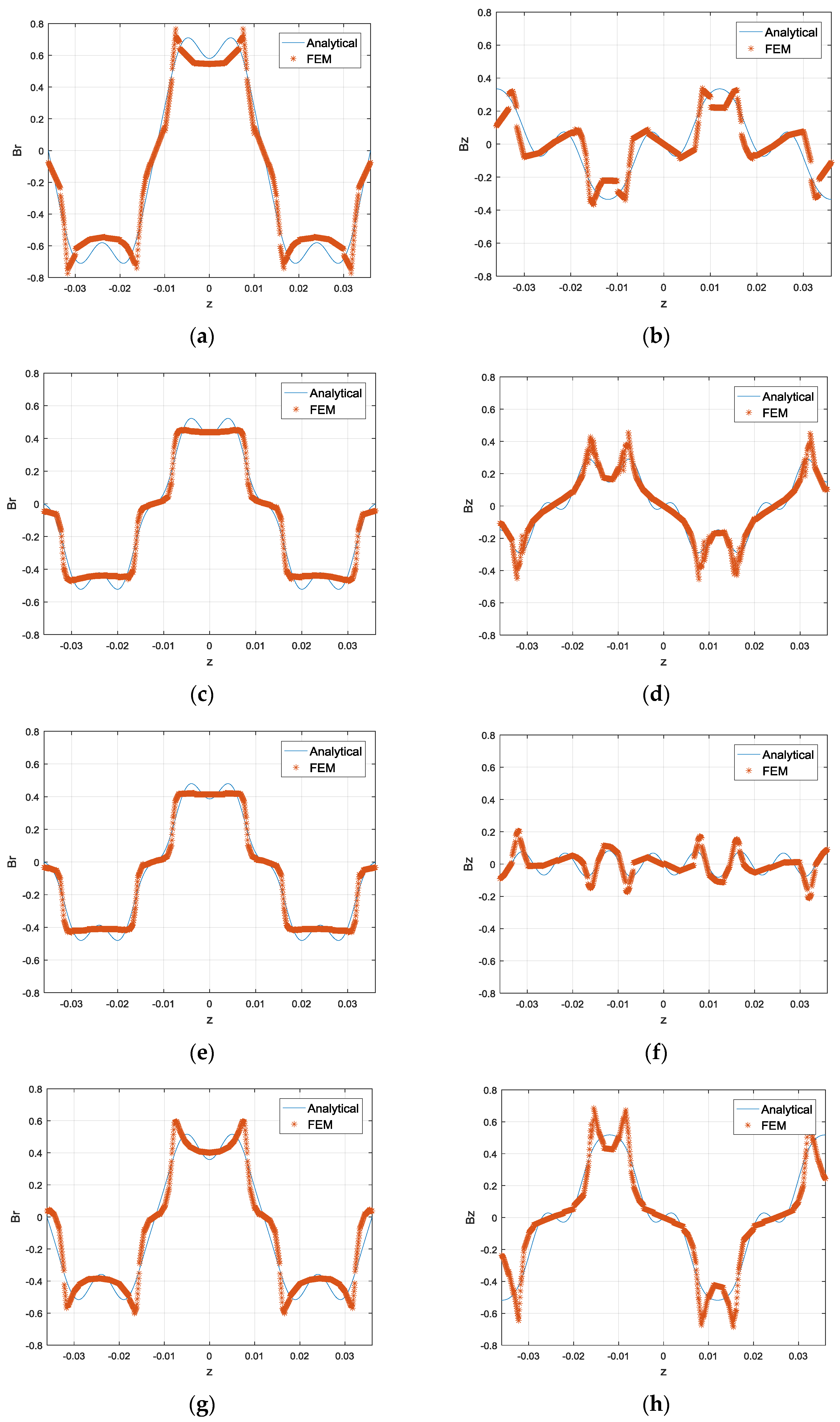
5.2. Validation of Analytical Models
6. Discussion
Acknowledgments
Author Contributions
Conflicts of Interest
References
- Kou, B.; Huang, X.; Wu, H.; Li, L. Thrust and thermal characteristics of electromagnetic launcher based on permanent magnet linear synchronous motors. In Proceedings of the 2008 14th Symposium on Electromagnetic Launch Technology, Victoria, BC, Canada, 10–13 June 2008; pp. 1–6. [Google Scholar]
- Musolino, A.; Rizzo, R.; Tripodi, E. The double-sided tubular linear induction motor and its possible use in the electromagnetic aircraft launch system. IEEE Trans. Plasma Sci. 2013, 41, 1193–1200. [Google Scholar] [CrossRef]
- Hellinger, R.; Mnich, P. Linear motor-powered transportation: History, present status, and future outlook. Proc. IEEE 2009, 97, 1892–1900. [Google Scholar] [CrossRef]
- Lu, Z.; Zhou, H.; Liu, P.; Liu, G.; Chen, L. Design and analysis of five-phase fault-tolerant radially magnetized tubular permanent magnet motor for active vehicle suspensions. In Proceedings of the 2016 19th International Conference on Electrical Machines and Systems (ICEMS), Chiba, Japan, 13–16 November 2016; pp. 1–4. [Google Scholar]
- Commins, P.A.; Moscrop, J.W.; Cook, C.D. Novel tooth design for a tubular linear motor for machine tool axis. In Proceedings of the 2011 IEEE International Conference on Mechatronics (ICM), Istanbul, Turkey, 13–15 Apirl 2011; pp. 660–665. [Google Scholar]
- Shukor, A.Z.; Fujimoto, Y. Direct-drive position control of a spiral motor as a monoarticular actuator. IEEE Trans. Ind. Electron. 2014, 61, 1063–1071. [Google Scholar] [CrossRef]
- Tang, X.; Lin, T.; Zuo, L. Design and optimization of a tubular linear electromagnetic vibration energy harvester. IEEE/ASME Trans. Mechatron. 2014, 19, 615–622. [Google Scholar] [CrossRef]
- Asama, J.; Burkhardt, M.R.; Davoodi, F.; Burdick, J.W. Investigation of energy harvesting circuit using a capacitor-sourced buck converter for a tubular linear generator of a moball: A spherical wind-driven exploration robot. In Proceedings of the 2015 IEEE Energy Conversion Congress and Exposition (ECCE), Montreal, QC, Canada, 20–24 September 2015; pp. 3167–3171. [Google Scholar]
- Slamani, M.; Nubiola, A.; Bonev, I.A. Effect of servo systems on the contouring errors in industrial robots. Trans. Can. Soc. Mech. Eng. 2012, 36, 83–96. [Google Scholar]
- Kwak, H.-J.; Park, G.-T. Study on the mobility of service robots. Int. J. Eng. Technol. Innov. 2012, 2, 97–112. [Google Scholar]
- Von Büren, T.; Tröster, G. Design and optimization of a linear vibration-driven electromagnetic micro-power generator. Sens. Actuators A Phys. 2007, 135, 765–775. [Google Scholar] [CrossRef]
- Kim, W.-J.; Murphy, B.C. Development of a novel direct-drive tubular linear brushless permanent-magnet motor. Int. J. Control Autom. Syst. 2004, 2, 279–288. [Google Scholar]
- Huang, X.; Tan, Q.; Wang, Q.; Li, J. Optimization for the Pole Structure of Slot-Less Tubular Permanent Magnet Synchronous Linear Motor and Segmented Detent Force Compensation. IEEE Trans. Appl. Supercond. 2016, 26, 0611405. [Google Scholar] [CrossRef]
- Wang, J.; Jewell, G.; Howe, D. Design optimisation and comparison of tubular permanent magnet machine topologies. IEE Proc. Electr. Power Appl. 2001, 148, 456–464. [Google Scholar] [CrossRef]
- Nirei, M.; Tang, Y.; Mizuno, T.; Yamamoto, H.; Shibuya, K.; Yamada, H. Iron loss analysis of moving-coil-type linear DC motor. Sens. Actuators A Phys. 2000, 81, 305–308. [Google Scholar] [CrossRef]
- Baloch, N.; Khaliq, S.; Kwon, B.-I. A High Force Density HTS Tubular Vernier Machine. IEEE Trans. Magn. 2017, 53, 8111205. [Google Scholar] [CrossRef]
- Wang, J.; Atallah, K.; Wang, W. Analysis of a magnetic screw for high force density linear electromagnetic actuators. IEEE Trans. Magn. 2011, 47, 4477–4480. [Google Scholar] [CrossRef]
- Halbach, K. Design of permanent multipole magnets with oriented rare earth cobalt material. Nuclear Instrum. Methods 1980, 169, 1–10. [Google Scholar] [CrossRef]
- Wang, J.; Jewell, G.W.; Howe, D. A general framework for the analysis and design of tubular linear permanent magnet machines. IEEE Trans. Magn. 1999, 35, 1986–2000. [Google Scholar] [CrossRef]
- Wang, T.; Jiao, Z.; Yan, L.; Chen, C.-Y.; Chen, I.-M. Design and analysis of an improved Halbach tubular linear motor with non-ferromagnetic mover tube for direct-driven EHA. In Proceedings of the 2014 IEEE Chinese Guidance, Navigation and Control Conference (CGNCC), Yantai, China, 8–10 August 2014; pp. 797–802. [Google Scholar]
- Abdalla, I.I.; Ibrahim, T.; Nor, N.M. Design and modeling of a single-phase linear permanent magnet motor for household refrigerator applications. In Proceedings of the 2013 IEEE Business Engineering and Industrial Applications Colloquium (BEIAC), Langkawi, Malaysia, 7–9 Apirl 2013; pp. 634–639. [Google Scholar]
- Zhang, L.; Yan, L.; Yao, N.; Wang, T.; Jiao, Z.; Chen, I.-M. Force formulation of a three-phase tubular linear machine with dual Halbach array. In Proceedings of the 2012 10th IEEE International Conference on Industrial Informatics (INDIN), Beijing, China, 25–27 July 2012; pp. 647–652. [Google Scholar]
- Yan, L.; Zhang, L.; Jiao, Z.; Hu, H.; Chen, C.-Y.; Chen, I.-M. A tubular linear machine with dual Halbach array. Eng. Comput. 2014, 31, 177–200. [Google Scholar] [CrossRef]
- Zhang, B.; Cheng, M.; Wang, J.; Zhu, S. Optimization and analysis of a yokeless linear flux-switching permanent magnet machine with high thrust density. IEEE Trans. Magn. 2015, 51, 8204804. [Google Scholar] [CrossRef]
- Wikipedia. Available online: https://en.wikipedia.org/wiki/Bessel_function (accessed on 9 November 2017).
- Wolframe MathWorld. Available online: http://mathworld.com/ModifiedStruveFunction.html (accessed on 9 November 2017).
- Ibala, A.; Masmoudi, A. Accounting for the armature magnetic reaction and saturation effects in the reluctance model of a new concept of claw-pole alternator. IEEE Trans. Magn. 2010, 46, 3955–3961. [Google Scholar] [CrossRef]
- Gaussens, B.; Hoang, E.; de la Barriere, O.; Saint-Michel, J.; Manfe, P.; Lecrivain, M.; Gabsi, M. Analytical armature reaction field prediction in field-excited flux-switching machines using an exact relative permeance function. IEEE Trans. Magn. 2013, 49, 628–641. [Google Scholar] [CrossRef]


| Magnet Patterns | Particular Designs | Features |
|---|---|---|
| Axial magnetization | Three magnets with axial magnetization | Simple structure, easy control; high flux leakage, low force output |
| NS-NS-SN-SN fashion with spacers | High flux density near the like pole regions, improve force output; low volume efficiency | |
| Convex magnet pole | Low magnetic saturation, low flux leakage; difficult fabrication and assembly | |
| Radial magnetization | Surface-mounted radial magnetization | Less magnet material, high dynamics; lower flux density, special magnetization fixture |
| Single ring magnet with multiple sectors | No special requirement of magnetization fixture; high flux leakage, low force output | |
| Multiple magnets in axial direction | High force output, large working range; magnetization and assembly challenge | |
| Magnetic screw-nut | Produce force and torque simultaneously; coupled motions in two directions | |
| Halbach array and its extension | Conventional Halbach array | High flux density on one side of PM; flux leakage exists although it is relatively reduced. |
| Improved compounded Halbach array | Good shielding effect, low mover mass, high dynamic response; difficult magnet assembly | |
| T-shaped and trapezoidal magnet | High magnetic flux linkage; Non-regular shape of magnets, difficult for fabrication | |
| Dual Halbach array | High axial force output, low radial vibration; Force enhancement is not significant, especially for large size machine. |
| Parameter Items | Value |
|---|---|
| Thickness of back iron, | 0.005(m) |
| Outer radius of inner Halbach layer, | 0.010(m) |
| Inner radius of middle PM layer, | 0.017(m) |
| Outer radius of middle PM layer, | 0.020(m) |
| Inner radius of outer Halbach layer, | 0.028(m) |
| Outer radius of outer Halbach layer, | 0.032(m) |
| Outer radius of outer back iron, | 0.035(m) |
| Width of radial magnets, | 0.016(m) |
| Width of axial magnets, | 0.008(m) |
| Pole pitch, | 0.024(m) |
| Permeability of vacuum, | |
| Relative permeability of PMs, | |
| Remenance, | 1.23(T) |
© 2017 by the authors. Licensee MDPI, Basel, Switzerland. This article is an open access article distributed under the terms and conditions of the Creative Commons Attribution (CC BY) license (http://creativecommons.org/licenses/by/4.0/).
Share and Cite
Yao, N.; Yan, L.; Wang, T.; Wang, S. Magnetic Flux Distribution of Linear Machines with Novel Three-Dimensional Hybrid Magnet Arrays. Sensors 2017, 17, 2662. https://doi.org/10.3390/s17112662
Yao N, Yan L, Wang T, Wang S. Magnetic Flux Distribution of Linear Machines with Novel Three-Dimensional Hybrid Magnet Arrays. Sensors. 2017; 17(11):2662. https://doi.org/10.3390/s17112662
Chicago/Turabian StyleYao, Nan, Liang Yan, Tianyi Wang, and Shaoping Wang. 2017. "Magnetic Flux Distribution of Linear Machines with Novel Three-Dimensional Hybrid Magnet Arrays" Sensors 17, no. 11: 2662. https://doi.org/10.3390/s17112662
APA StyleYao, N., Yan, L., Wang, T., & Wang, S. (2017). Magnetic Flux Distribution of Linear Machines with Novel Three-Dimensional Hybrid Magnet Arrays. Sensors, 17(11), 2662. https://doi.org/10.3390/s17112662