Radar Constant-Modulus Waveform Optimization for High-Resolution Range Profiling of Stationary Targets

Abstract
:1. Introduction
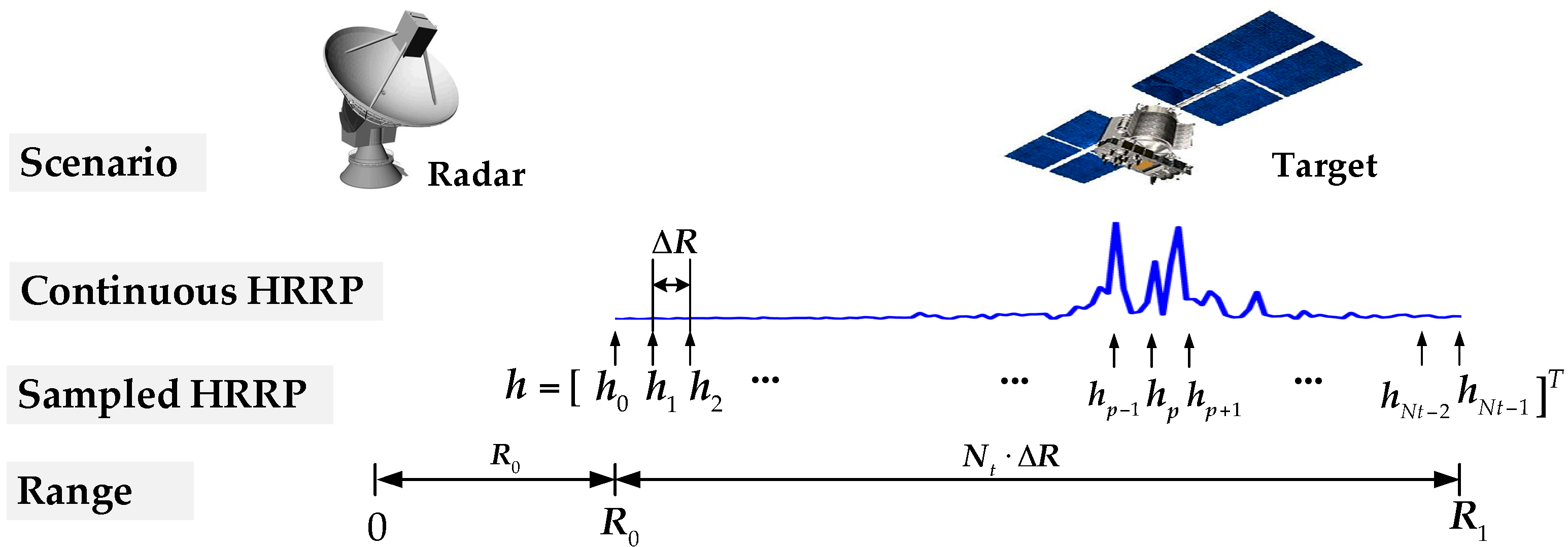
2. Signal Model
3. Performance Analysis of HRR Profiling
3.1. Unambiguous Criterion
3.2. Upper Bound of the Profiling Error
3.3. Lower Bound of the Profiling Error
4. Constant-Modulus Waveform Design
4.1. Problem Analysis
4.2. CM Waveform Design
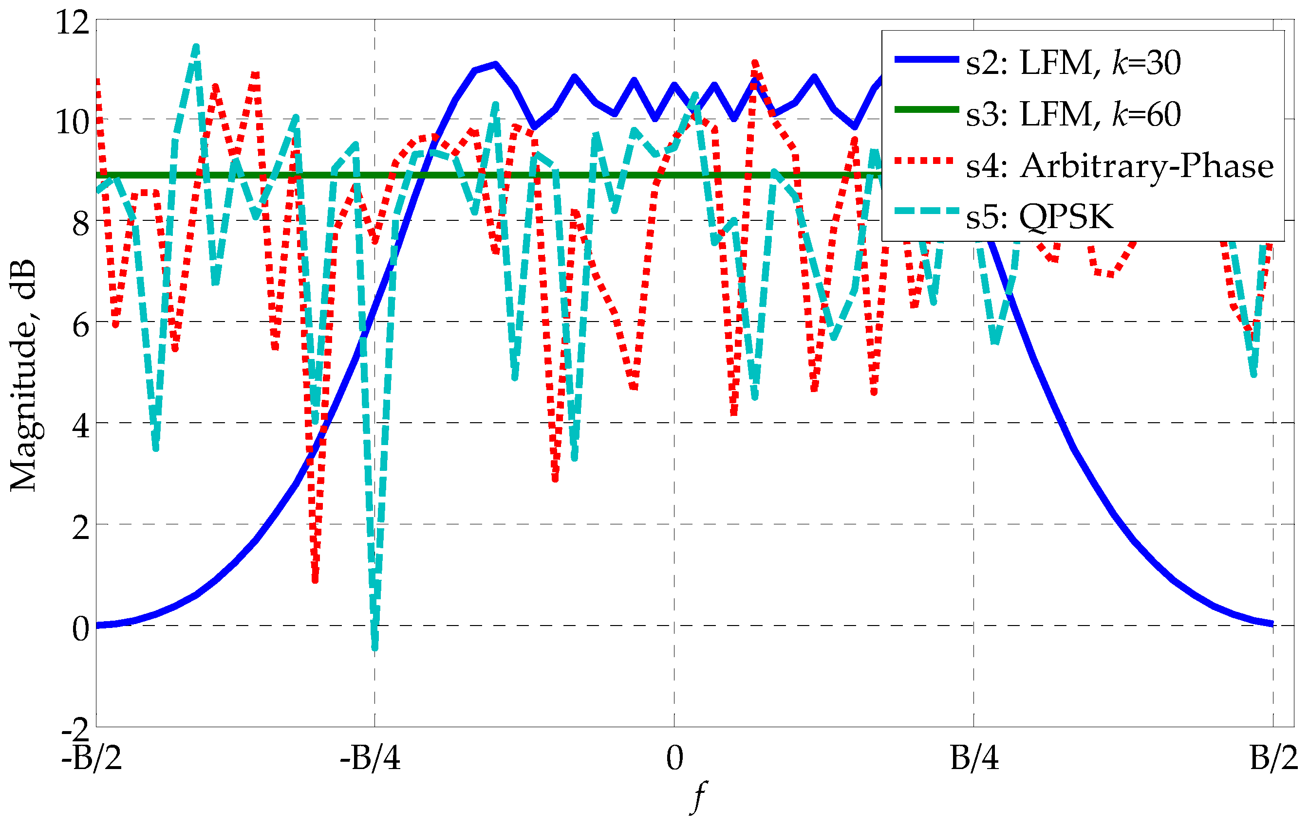
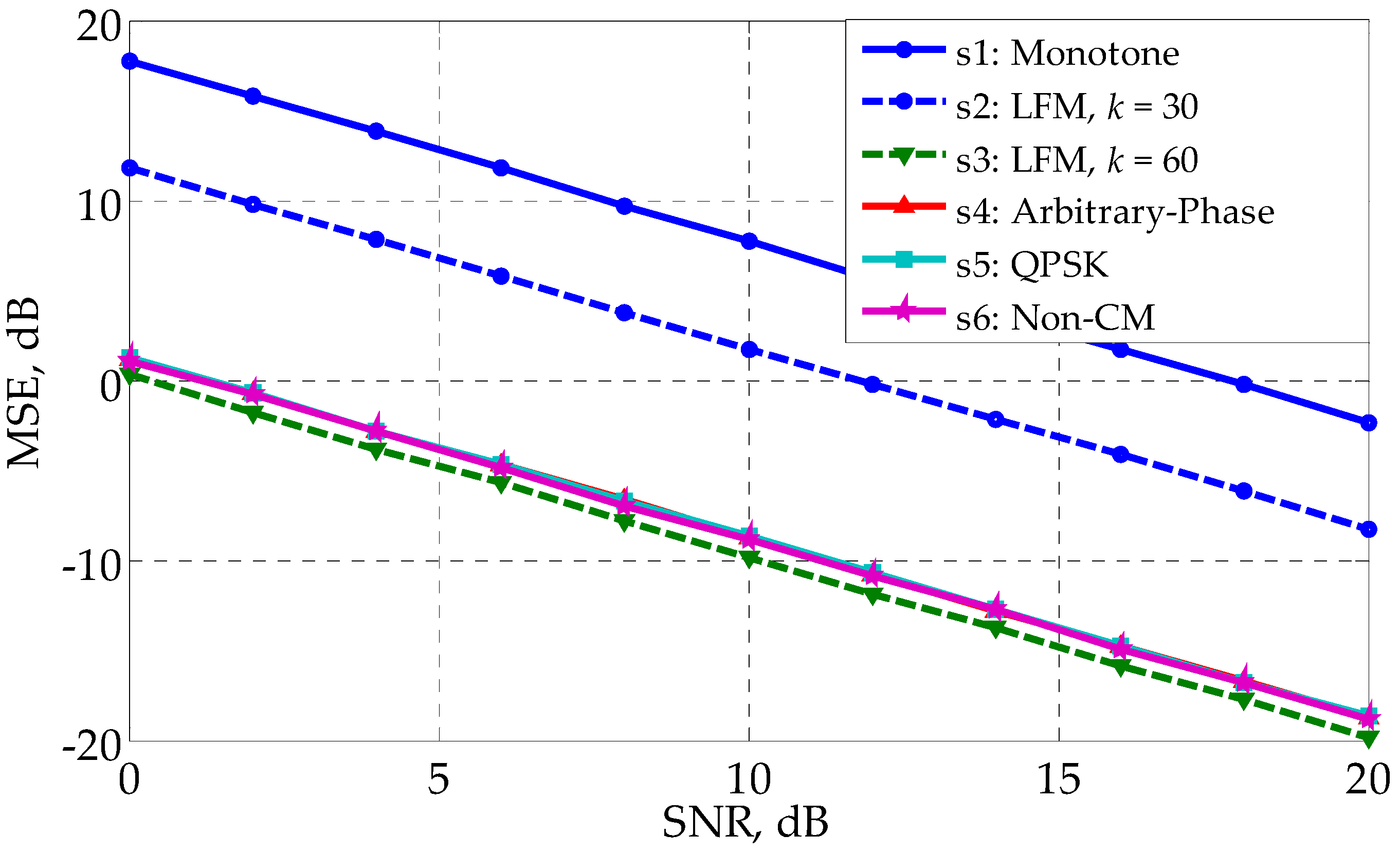
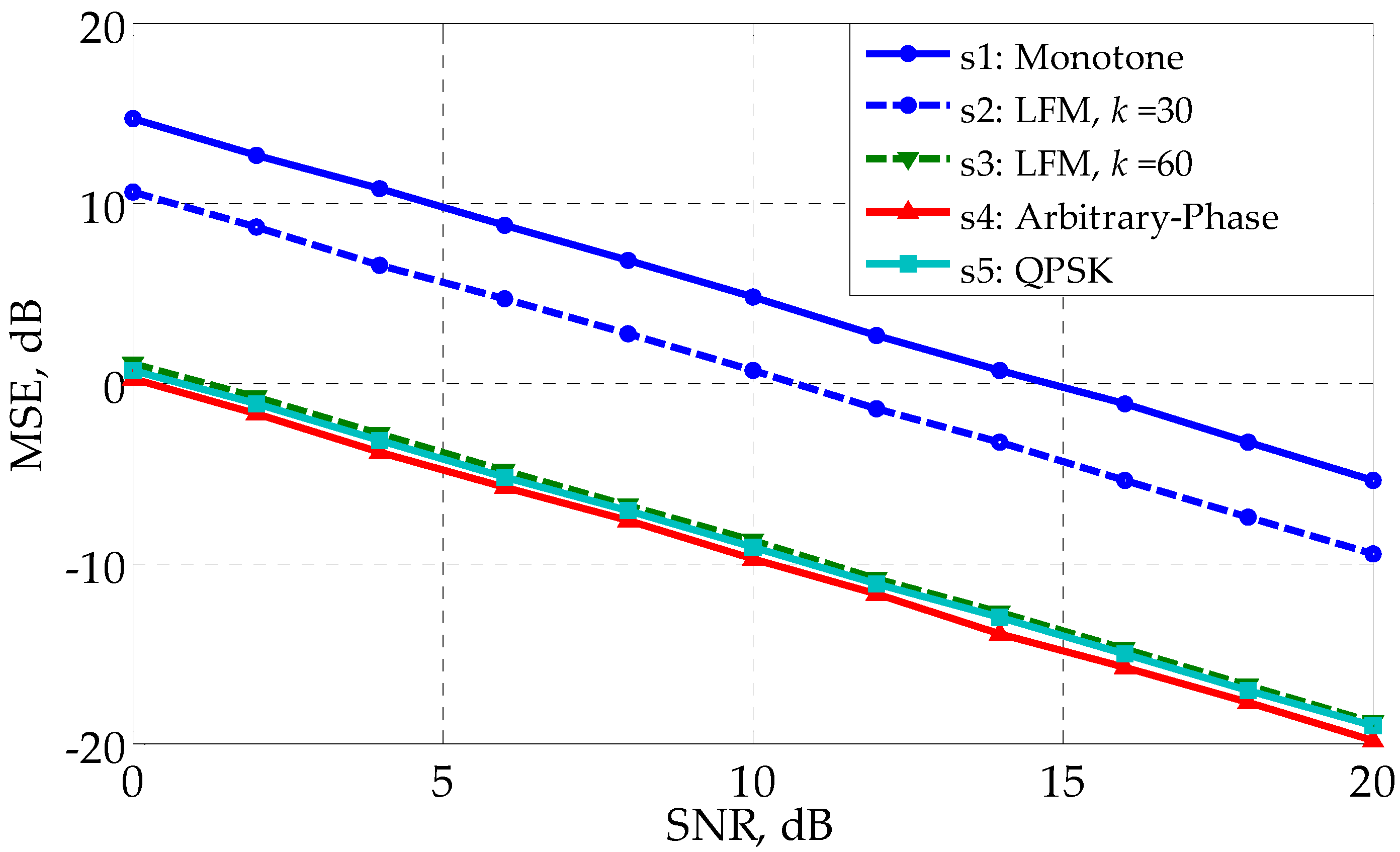
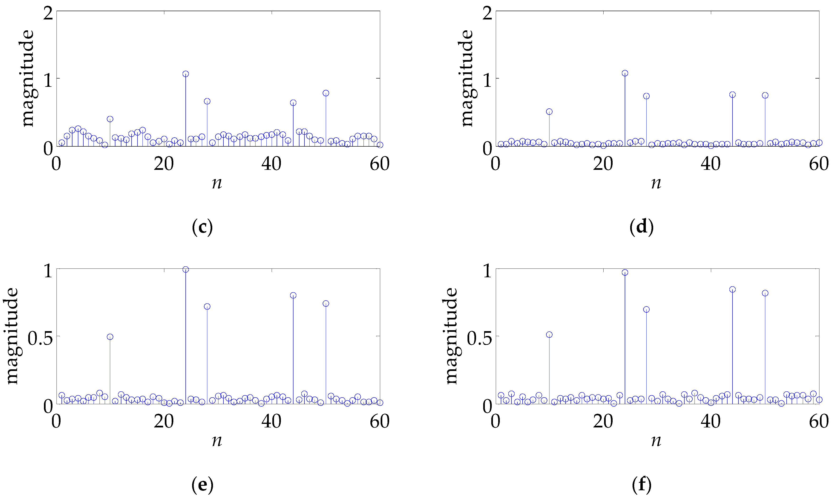
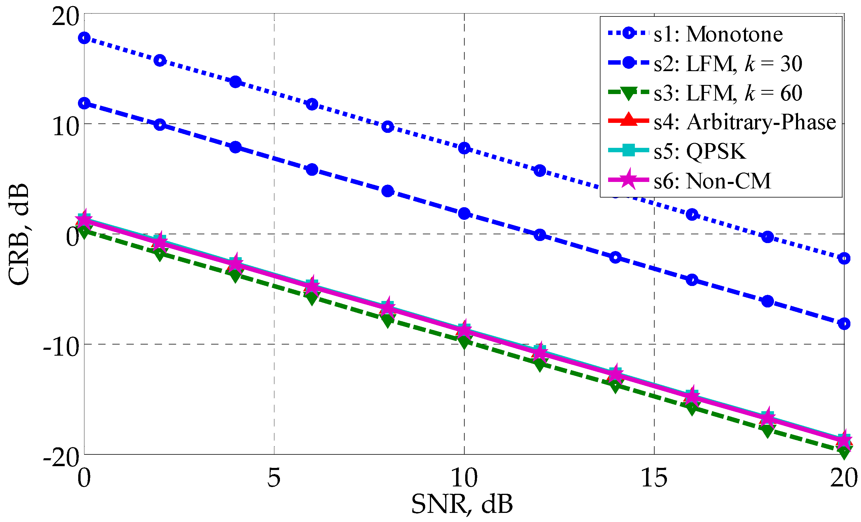
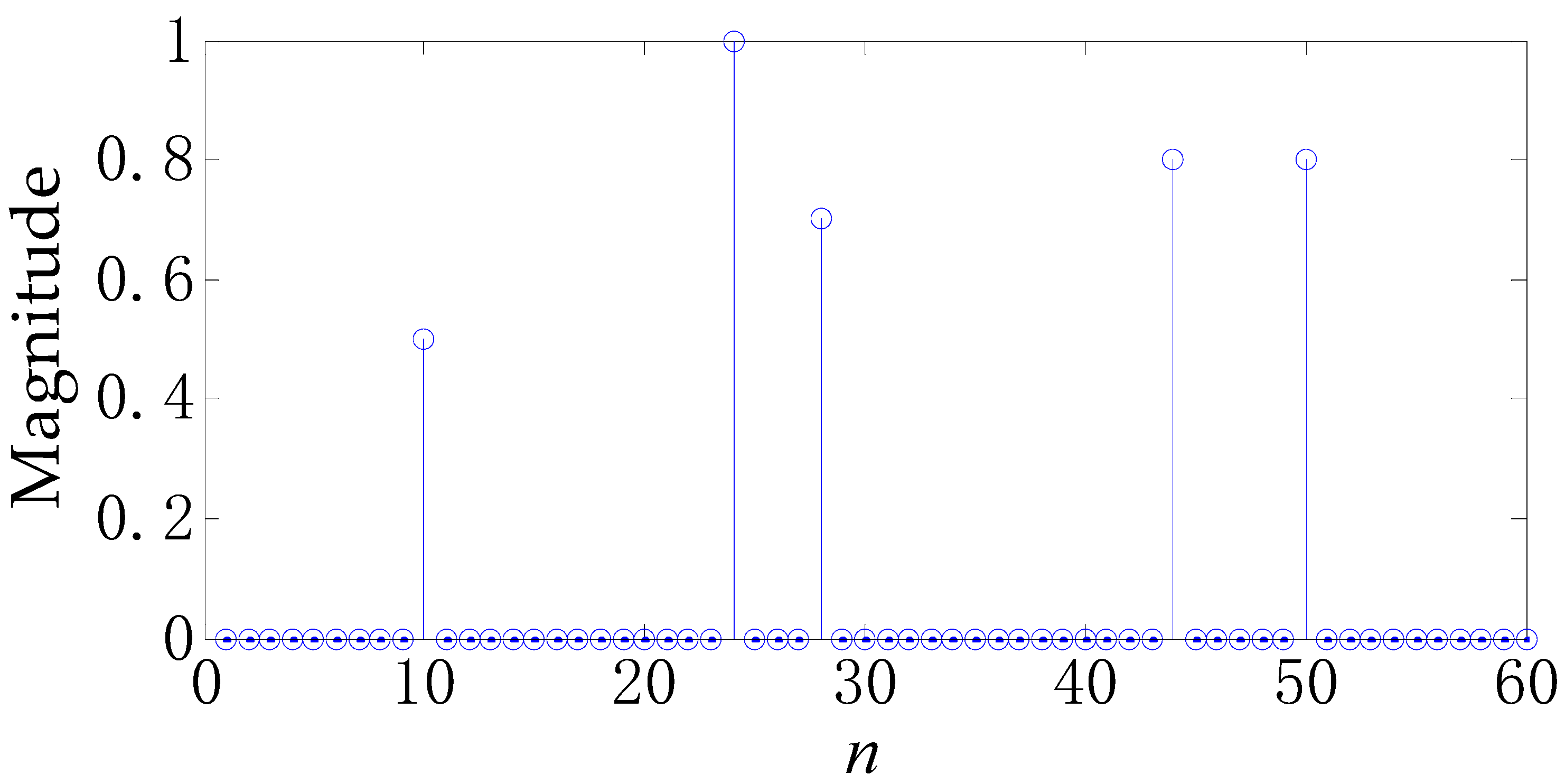
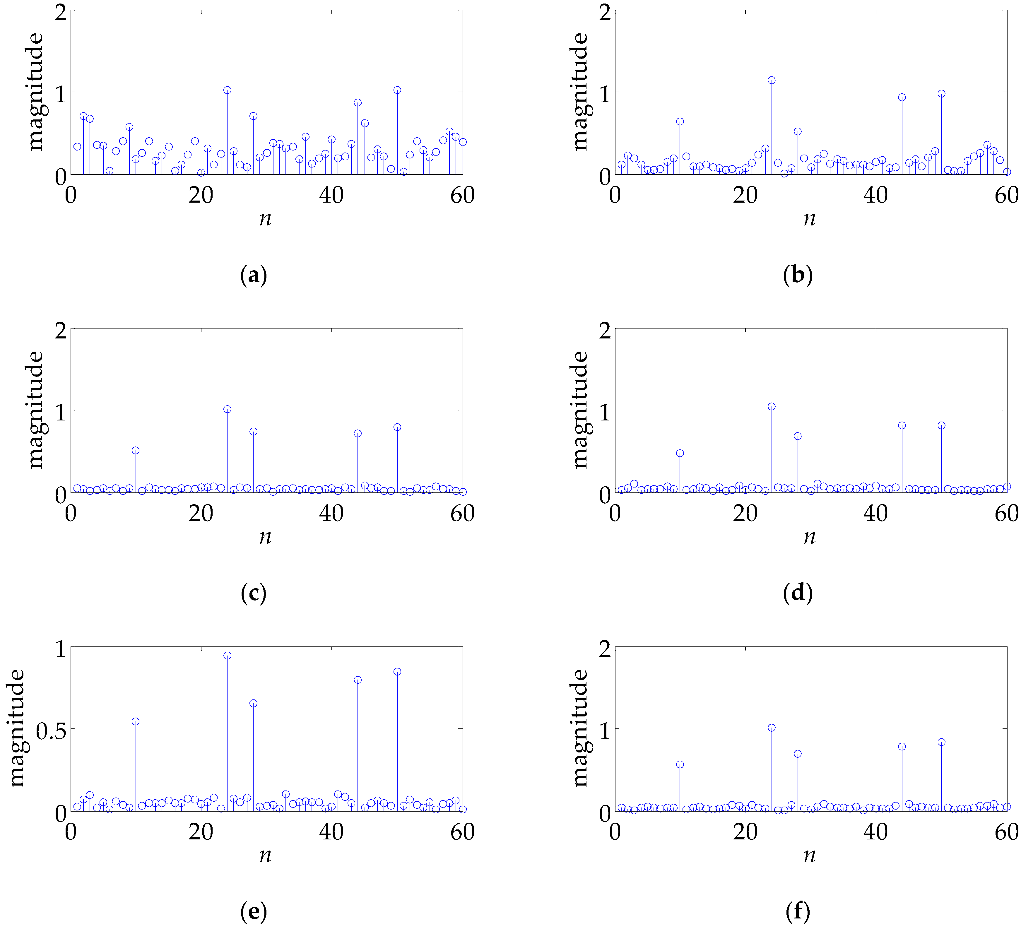
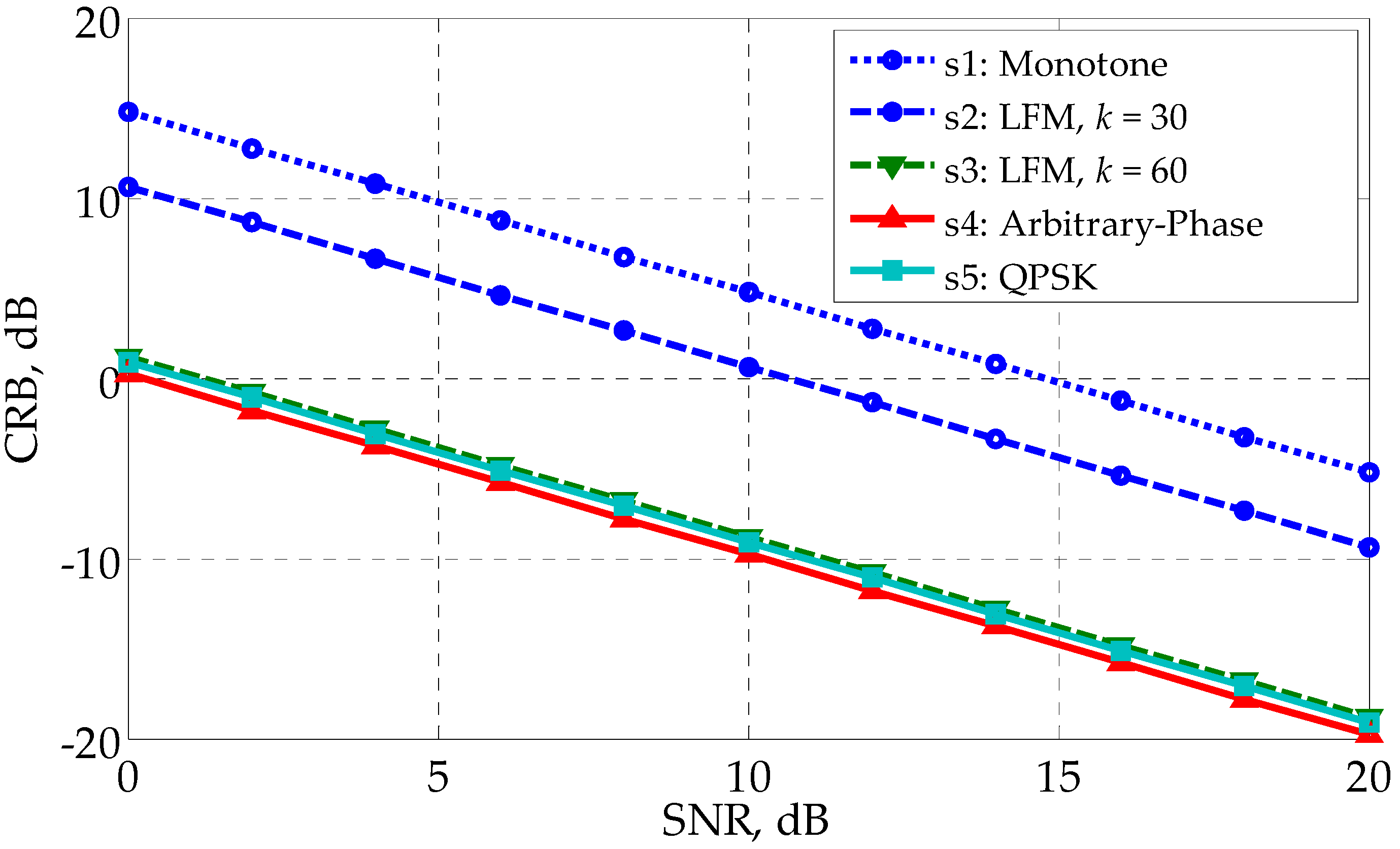
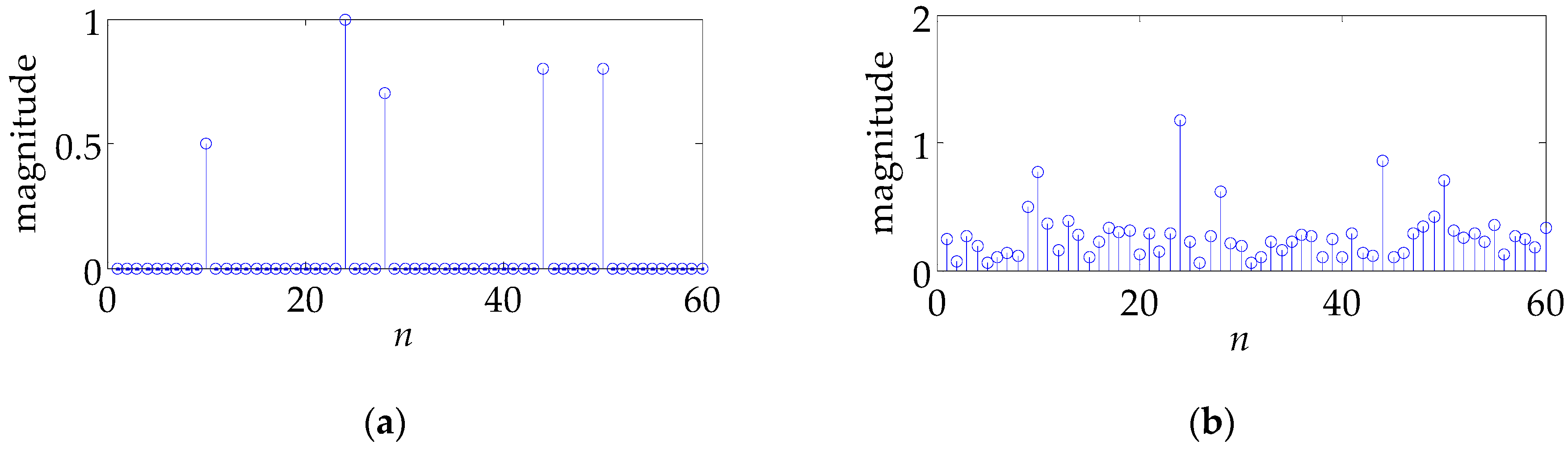
5. Simulation Results
5.1. White Noise Case
5.2. Colored Noise Case
6. Conclusions
Acknowledgments
Author Contributions
Conflicts of Interest
Appendix A. Proof of Theorem 1
- (a)
- is full-column rank.
- (b)
- has to be a zero vector to make , i.e., .
- (c)
- has to be an all-zero vector to make .
- (d)
- Matrix is full-rank.
- (e)
- . In other words, there is no zero element in the vector .
Appendix B. Proof of Theorem 2
Appendix C. Derivation of an Upper Bound of the CRB
References
- Richards, M.A. Fundamentals of Radar Signal Processing; McGraw-Hill Education: New York, NY, USA, 2005; pp. 385–455. [Google Scholar]
- Peng, X.; Gao, X.; Zhang, Y.; Li, X. An Adaptive feature learning model for sequential radar high resolution range profile recognition. Sensors 2017, 17, 1675. [Google Scholar] [CrossRef] [PubMed]
- Du, L.; Liu, H.; Wang, P.H.; Bo, F.; Pan, M.; Bao, Z. Noise robust radar HRRP target recognition based on multitask factor analysis with small training data size. IEEE Trans. Signal Process. 2012, 60, 3546–3559. [Google Scholar]
- Goodman, N.A.; Venkata, P.R.; Neifeld, M.A. Adaptive waveform design and sequential hypothesis testing for target recognition with active sensors. IEEE J. Sel. Top. Signal Process. 2007, 1, 105–113. [Google Scholar] [CrossRef]
- Romero, R.A.; Goodman, N.A. Waveform design in signal-dependent interference and application to target recognition with multiple transmissions. IET Radar Sonar Navig. 2009, 3, 328–340. [Google Scholar] [CrossRef]
- Liu, J.; Fang, N.; Xie, Y.J.; Wang, B.F. Scale-space theory-based multi-scale features for aircraft classification using HRRP. IET Electron. Lett. 2016, 52, 475–477. [Google Scholar] [CrossRef]
- Zyweck, A.; Bogner, R.E. Radar target classification of commercial aircraft. IEEE Trans. Aerosp. Electron. Syst. 1996, 32, 598–606. [Google Scholar] [CrossRef]
- Chen, C.Y.; Vaidyanathan, P.P. MIMO radar waveform optimization with prior information of the extended target and clutter. IEEE Trans. Signal Process. 2009, 57, 3533–3544. [Google Scholar] [CrossRef]
- Yue, W.Z.; Zhang, Y.; Liu, Y.M.; Xie, J.W. Radar constant-modulus waveform design with prior information of the extended target and clutter. Sensors 2016, 16, 889. [Google Scholar] [CrossRef] [PubMed]
- Liu, Y.M.; Huang, T.; Meng, H.D.; Wang, X.Q. Fundamental limits of HRR profiling and velocity compensation for stepped-frequency waveforms. IEEE Trans. Signal Process. 2014, 62, 4490–4504. [Google Scholar] [CrossRef]
- Huang, T.Y.; Liu, Y.M.; Meng, H.D.; Wang, X.Q. Cognitive random stepped frequency radar with sparse recovery. IEEE Trans. Aerosp. Electron. Syst. 2014, 50, 858–870. [Google Scholar] [CrossRef]
- Stoica, P.; Li, J.; Zhu, X. Waveform synthesis for diversity-based transmit beampattern design. IEEE Trans. Signal Process. 2008, 56, 2593–2598. [Google Scholar] [CrossRef]
- Bell, M.R. Information theory and radar waveform design. IEEE Trans. Inf. Theory 1993, 39, 1578–1597. [Google Scholar] [CrossRef]
- Yang, Y.; Blum, R.S. MIMO radar waveform design based on mutual information and minimum mean-square error estimation. IEEE Trans. Aerosp. Electron. Syst. 2007, 43, 330–343. [Google Scholar] [CrossRef]
- Yang, Y.; Blum, R.S. Minimax robust MIMO radar waveform design. IEEE J. Sel. Top. Signal Process. 2007, 1, 147–155. [Google Scholar] [CrossRef]
- Leshem, A.; Naparstek, O.; Nehorai, A. Information theoretic adaptive radar waveform design for multiple extended targets. IEEE J. Sel. Top. Signal Process. 2007, 1, 42–55. [Google Scholar] [CrossRef]
- Sira, S.P.; Cochran, D.; Papandreou, S.A. Adaptive waveform design for improved detection of low-RCS targets in heavy sea clutter. IEEE J. Sel. Top. Signal Process. 2007, 1, 56–66. [Google Scholar] [CrossRef]
- Aubry, A.; de Maio, A.; Jiang, B. Ambiguity function shaping for cognitive radar via complex quartic optimization. IEEE Trans. Signal Process. 2013, 61, 5603–5619. [Google Scholar] [CrossRef]
- Chitgarha, M.M.; Radmard, M.; Majd, M.N.; Karbasi, S.M.; Nayebi, M.M. MIMO radar signal design to improve the MIMO ambiguity function via maximizing its peak. Signal Process. 2016, 118, 139–152. [Google Scholar] [CrossRef]
- Li, F.C.; Zhao, Y.N.; Qiao, X.L. A waveform design method for suppressing range sidelobes in desired intervals. Signal Process. 2014, 96, 203–211. [Google Scholar] [CrossRef]
- Zhang, J.D.; Zhu, X.; Wang, H.Q. Adaptive radar phase-coded waveform design. IET Electron. Lett. 2009, 45, 1052–1053. [Google Scholar] [CrossRef]
- Pillai, S.U.; Oh, H.S.; Youla, D.C.; Guerci, J.R. Optimum transmit-receiver design in the presence of signal-dependent interference and channel noise. IEEE Trans. Inf. Theory 2000, 46, 577–584. [Google Scholar] [CrossRef]
- Jiu, B.; Liu, H.; Zhang, L.; Wang, Y.; Luo, T. Wideband cognitive radar waveform optimization for joint target radar signature estimation and target detection. IEEE Trans. Aerosp. Electron. Syst. 2015, 51, 1530–1546. [Google Scholar] [CrossRef]
- Gong, X.; Meng, H.; Wei, Y.; Wang, X. Phase-modulated waveform design for extended target detection in the presence of clutter. Sensors 2011, 11, 7162–7177. [Google Scholar] [CrossRef] [PubMed]
- Cheng, X.; Aubry, A.; Ciuonzo, D. Optimizing polarimetrie radar waveform and filter bank for extended targets in clutter. In Proceedings of the Sensor Array and Multichannel Signal Processing Workshop (SAM), Rio de Janerio, Brazil, 10–13 July 2016; pp. 1–5. [Google Scholar]
- Cheng, X.; Aubry, A.; Ciuonzo, D.; De Maio, A.; Wang, X. Robust waveform and filter bank design of polarimetric radar. IEEE Trans. Aerosp. Electron. Syst. 2017, 53, 370–384. [Google Scholar] [CrossRef]
- Garren, D.A.; Odom, A.C.; Osborn, M.K. Full-polarization matched-illumination for target detection and identification. IEEE Trans. Aerosp. Electron. Syst. 2002, 38, 824–837. [Google Scholar] [CrossRef]
- Ciuonzo, D.; De Maio, A.; Foglia, G.; Piezzo, M. Intrapulse radar-embedded communications via multiobjective optimization. IEEE Trans. Aerosp. Electron. Syst. 2015, 51, 2960–2974. [Google Scholar] [CrossRef]
- Jiang, N.Z.; Wu, R.B.; Li, J. Super resolution feature extraction of moving targets. IEEE Trans. Aerosp. Electron. Syst. 2001, 37, 781–793. [Google Scholar] [CrossRef]
- Stoica, P.; Moses, R.L. Introduction to Spectral Analysis; Prentice Hall: Upper Saddle River, NJ, USA, 1997; pp. 285–297. [Google Scholar]
- Huang, T.Y.; Liu, Y.; Meng, H.; Wang, X. Adaptive compressed sensing via minimizing Cramer–Rao bound. IEEE Signal Process. Lett. 2014, 21, 270–274. [Google Scholar] [CrossRef]
- Yue, W.Z.; Zhang, Y.; Xie, J.W. QPSK signal design for given correlation matrix. IET Electron. Lett. 2016, 52, 399–401. [Google Scholar] [CrossRef]
- Zhang, X. Matrix Analysis and Applications, 2nd ed.; Tsinghua University Press: Beijing, China, 2013; pp. 67–74. [Google Scholar]
- Böttcher, A.; Grudsky, S.M. On the condition numbers of large semidefinite Toeplitz matrices. Linear Algebra Its Appl. 1998, 279, 285–301. [Google Scholar] [CrossRef]


| Step 1: Obtain a series of non-CM Gaussian-distributed vectors (denoted as ) to realize the covariance matrix X. The step can be done by means of the Cholesky factorization or eigenvalue decomposition. |
| Step 2: Get the CM vector by normalizing the modulus of , . can be seen as the candidate vector for . |
| Step 3: Choose the candidate vector that minimizes Equation (28). For the white noise case, is Equation (27); for the colored noise case, is generated from in Equation (32). |
| Step 1: Denote the real and imaginary parts of by and , respectively. |
| Step 2: Generate via |
| Step 3: Make a forced positive definite Cholesky decomposition . D is a diagonal matrix with nonnegative elements. |
| Step 4: Let , where is a Gaussian distributed vector with zero mean and unit variance. The QPSK vector can then be generated by |
| Step 5: Generate a series of QPSK candidate vectors via the preceding steps, and choose the one that minimizes Equation (28). |
| Computational Complexity | CM Waveform Design | QPSK Waveform Design |
|---|---|---|
| White noise | ||
| Colored noise |
© 2017 by the authors. Licensee MDPI, Basel, Switzerland. This article is an open access article distributed under the terms and conditions of the Creative Commons Attribution (CC BY) license (http://creativecommons.org/licenses/by/4.0/).
Share and Cite
Yue, W.; Li, L.; Xin, Y.; Han, T. Radar Constant-Modulus Waveform Optimization for High-Resolution Range Profiling of Stationary Targets. Sensors 2017, 17, 2574. https://doi.org/10.3390/s17112574
Yue W, Li L, Xin Y, Han T. Radar Constant-Modulus Waveform Optimization for High-Resolution Range Profiling of Stationary Targets. Sensors. 2017; 17(11):2574. https://doi.org/10.3390/s17112574
Chicago/Turabian StyleYue, Wenzhen, Lin Li, Yu Xin, and Tao Han. 2017. "Radar Constant-Modulus Waveform Optimization for High-Resolution Range Profiling of Stationary Targets" Sensors 17, no. 11: 2574. https://doi.org/10.3390/s17112574
APA StyleYue, W., Li, L., Xin, Y., & Han, T. (2017). Radar Constant-Modulus Waveform Optimization for High-Resolution Range Profiling of Stationary Targets. Sensors, 17(11), 2574. https://doi.org/10.3390/s17112574