The Application of EM38: Determination of Soil Parameters, Selection of Soil Sampling Points and Use in Agriculture and Archaeology


Abstract
:1. Introduction
2. Goal of this Study
- Salinity
- Soil-related properties in non-saline soils
- Soil texture
- Soil water content, water balance
- Soil horizons and vertical discontinuities
- N-turnover, cation exchange capacity, organic matter and additional soil parameters
- Soil sampling designs
- Soil type boundaries
- Agriculture
- Agricultural yield variability and management zones
- Efficiency of agricultural field experimentation
- Additional application of EM38 in agriculture and horticulture
- Archaeology
3. Surveying Soil Salinity
- Leached soils, where salinity increases with depth, defined by ECah/ECav ≤ 1.0
- Uniform, where salinity does not change significantly with profile depth and where 1.0 < ECah/ECav ≤ 1.05, and
- Inverted salinity profiles, where salinity decreases with depth and where ECah/ECav > 1.05.
4. Detecting Soil-Related Properties in Non-Saline Soils by EM-38
4.1. Influence of Soil Water Content Conditions
4.2. Soil Texture
4.3. Soil Water Content, Water Balance
4.4. Detection of Soil Horizons and Vertical Discontinuities
4.5. Relationships to N-turnover, Cation Exchange Capacity, Organic Matter and Additional Soil Parameters
4.6. Derivation of Soil Sampling Designs
4.7. Derivation of Soil Type Boundaries
5. Applications in Agriculture
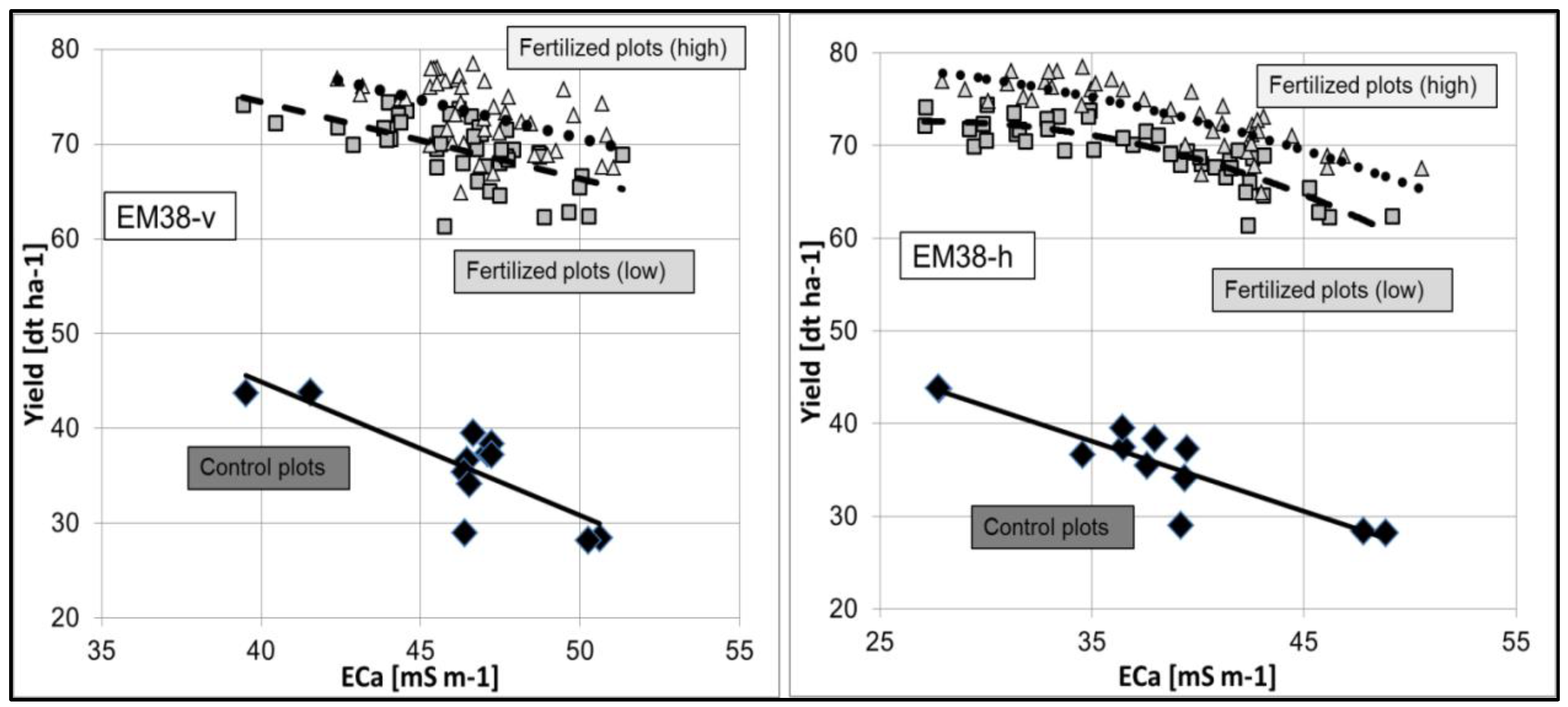
5.1. Derivation of Agricultural Yield Variability and Management Zones
- The spatial distribution of the yield was at first influenced by the ECa across the field. Treatment effects (fertilizing level, fertilizer form) were overlain by soil conditions with different ECa values.
- The height of the yield was secondly assumedly determined by the level of fertilization.
5.2. Improvement of the Efficiency of Agricultural Field Experimentation
5.3. Additional Application of EM38 in Agriculture and Horticulture
6. Application of EM38 in Archaeology
7. Conclusions and Closing Remarks
- The interpretation and utility of ECa readings are highly location and soil-specific; the soil properties contributing to ECa measurements must be clearly understood. From the various calibration results, it appears that regression constants for relationships between ECa, ECe, soil texture, yield, etc. are not necessarily transferable from one region to another. Several factors affect the strength of the signal and therefore, the relationships. In addition to texture, salt concentration and other physicochemical properties, calibrations are further affected by the relative response of the signal according to depth, the non-linearity of the signal and the collinearity between horizontal and vertical readings. The soil parameter with the greatest influence on ECa is also the best derivable.
- Only a few authors [108,196] account for the influence of the farming system, crop biomass, applications of fertilizer at the time of measurement on ECa distributions. Most of the identified soil parameters that influence ECa have significant interdependency and can thus provide multivariate effects on ECa.
- The modelling of ECa, soil properties, climate and yield are important for identifying the geographic extent to which specific applications of ECa technology (e.g., ECa – texture relationships) can be appropriately applied.
- In the case of detecting salinity, obviously better results are achieved if both EM38 readings (vertical and horizontal) are combined with ECe values from different depth ranges. Nevertheless, Vlotman et al. [37] posed the question about the need for converting the ECe from ECa. As McKenzie [24,25] showed, a classification of salinity tolerance level of different crops is also possible only with EM38 readings. A partitioning in areas of low, medium and high salinity with measurements in a single mode or with a combination of v- and h-mode is often a sufficient inventory of the salinity distribution. But it is necessary to take into account, that on the one field e.g., 60 mS m−1 has salt problems while another field with the same reading does not have such problems. Therefore ECe will continue to be important at least in the near future.
- The quality of a regression is often determined by a sufficient range of dependent and independent variables. Delin and Söderström [124] noted that when the ECa data were correlated with the clay content over the whole farm, the result was much better then when the correlation was restricted to single zones. This quality is also better if the target variable is also the dominant ECa-influencing factor.
- The construction of soil sampling designs with ECa readings is limited to those properties that correlate with ECa. Other parameters require some other sampling approach such as random, grid, or stratified random sampling.
- It seems that the detection of salinity is still the main area of application.
- Site-specific management in agriculture with the application of ECa is still in Germany in an initial phase of adoption among farmers. Predicting the future is difficult. Nonetheless, a greater presence of site-specific crop management based on soil detection is to be hoped for.
- Furthermore in Germany increases the investigations in improving soil maps and in detecting soil functions, including: plant available water, sorption capacity, binding strength for heavy metals, filtering of unbound substances and natural soil fertility. Additionally, soil protection measures are also indicators for erosion prevention, retention of nutrients, and conservation/enhancement of carbon contents (based on good agricultural practice after Article 17, German Soil Protection Act). The selection of soil functions is based on the German Soil Protection Act (LABO—Bund-Länder-Arbeitsgemeinschaft Bodenschutz). Here it is not common sense to carry out this also with EM38. Until now it is not well known that, compared to traditional soil survey methods, EM38 readings can more effectively characterize diffuse soil boundaries and identify areas of similar soils within mapped soil units. This gives soil scientists greater confidence in their soil mapping.
- The application in forests is world-wide rather seldom. But also here is an enormous potential to improve the existing site maps and to test the water distribution between the trees.
- The improvement of evaluation of field experiments with ECa readings as covariate is more rarely used. The spatial variability of soil properties can have adverse effects on the accuracy and efficiency of field experiments. Here is a great potential to take into account the soil conditions by using ECa readings.
- The fusion of the data of other sensors also shows great potential. The idea behind the combination of proximal soil sensors is that the accuracy of a single sensor is often not sufficient. The reading of one sensor is affected by more than one soil property of interest. The fusion of sensor data can overcome this weakness by extracting complementary information from multiple sensors or sources. Until now to an increasing extent, the readings of EM38 are evaluated in combination mainly with VIS–NIR and a gamma-ray-spectrometer.
- Many of the instruments measure at the point or sample scale, such as soil moisture probes and tensiometers, while remote sensing devices determine regional patterns. But these techniques are limited in the depth of penetration into the subsurface.
Acknowledgments
Conflicts of Interest
Abbreviations
| CEC | Cation exchange capacity |
| ECa | Apparent electrical conductivity |
| ECav | Apparent electrical conductivity, measured in vertical mode |
| ECah | Apparent electrical conductivity, measured in horizontal mode |
| ECe | Electrical conductivity of aqueous soil extracts EC1:5, EC1:2 or EC1:1, soil/water suspensions) |
| ECp | ECa calculated by using predictive equations |
| ECref | Quotient of the measured ECa and the EC |
| θv, θw | Weighted water content after vertical and horizontal mode |
| Z | Soil depth |
References
- Sudduth, K.A.; Drummond, S.T.; Kitchen, N.R. Accuracy issues in electromagnetic induction sensing of soil electrical conductivity for precision agriculture. Comput. Electron. Agric. 2001, 31, 239–264. [Google Scholar] [CrossRef]
- Doolittle, J.A.; Brevik, E.C. The use of electromagnetic induction techniques in soils studies. Geoderma 2014, 223–225, 33–45. [Google Scholar] [CrossRef]
- Sudduth, K.A.; Kitchen, N.R.; Wiebold, W.J.; Batchelor, W.D. Relating apparent electrical conductivity to soil properties across the north-central USA. Comput. Electron. Agric. 2005, 46, 263–283. [Google Scholar] [CrossRef]
- Heil, K.; Schmidhalter, U. Comparison of the EM38 and EM38-MK2 electromagnetic induction-based sensors for spatial soil analysis at field scale. Comput. Electron. Agric. 2015, 110, 267–280. [Google Scholar] [CrossRef]
- McNeill, J. Electromagnetic Terrain Conductivity Measurement at Low Induction Numbers. Available online: http://www.geonics.com/pdfs/technicalnotes/tn6.pdf (accessed on 1 November 2017).
- Geonics Limited. Ground Conductivity Meters. Available online: http://www.geonics.com/html/conductivitymeters.html (accessed on 15 August 2017).
- Corwin, D.L.; Lesch, S.M. Apparent soil electrical conductivity measurements in agriculture. Comput. Electron. Agric. 2005, 46, 11–43. [Google Scholar] [CrossRef]
- Cassel, F.; Goorahoo, D.; Sharmasarkar, S. Salinization and Yield Potential of a Salt-Laden Californian Soil: An In Situ Geophysical Analysis. Water Air Soil Pollut. 2015, 226, 1–8. [Google Scholar] [CrossRef]
- Cook, P.G.; Walker, G.R. Depth Profiles of Electrical-Conductivity from Linear-Combinations of Electromagnetic Induction Measurements. Soil Sci. Soc. Am. J. 1992, 56, 1015–1022. [Google Scholar] [CrossRef]
- Corwin, D.; Rhoades, J. An improved technique for determining soil electrical conductivity-depth relations from above-ground electromagnetic measurements. Soil Sci. Soc. Am. J. 1982, 46, 517–520. [Google Scholar] [CrossRef]
- Corwin, D.; Rhoades, J. Measurement of inverted electrical conductivity profiles using electromagnetic induction. Soil Sci. Soc. Am. J. 1984, 48, 288–291. [Google Scholar] [CrossRef]
- Dang, Y.P.; Dalal, R.C.; Pringle, M.J.; Biggs, A.J.W.; Darr, S.; Sauer, B.; Moss, J.; Payne, J.; Orange, D. Electromagnetic induction sensing of soil identifies constraints to the crop yields of north-eastern Australia. Soil Res. 2011, 49, 559–571. [Google Scholar] [CrossRef]
- Doolittle, J.; Petersen, M.; Wheeler, T. Comparison of two electromagnetic induction tools in salinity appraisals. J. Soil Water Conserv. 2001, 56, 257–262. [Google Scholar]
- Dunn, G.; Taylor, D.; Nester, M.; Beetson, T. Performance of twelve selected Australian tree species on a saline site in southeast Queensland. For. Ecol. Manag. 1994, 70, 255–264. [Google Scholar] [CrossRef]
- Ghany, A.H.; Omara, A.M.; El Nagar, M.A. Testing Electromagnetic Induction Device (EM 38) Under Egyptian Conditions; Vlotman, W.F., Ed.; EM38 Workshop: New Delhi, India, 2000. [Google Scholar]
- Gill, H.S.; Yee, M. EM-38 for Assessing Surface and Sub-Soil Salinity and Its Relationship to Establishment and Growth of Selected Perennial Pasture Species. In Proceedings of the SuperSoil 2004—3rd Australian New Zealand Soils Conference, Sydney, Australia, 5–9 December 2004. [Google Scholar]
- Herrero, J.; Ba, A.; Aragüés, R. Soil salinity and its distribution determined by soil sampling and electromagnetic techniques. Soil Use Manag. 2003, 19, 119–126. [Google Scholar] [CrossRef]
- Li, H.; Li, F.; Shi, Z.; Huang, M. Three Dimensional Variability of Soil Electrical Conductivity Based on Electromagnetic Induction Approach. In Proceedings of the 2010 International Conference on Artificial Intelligence and Computational Intelligence (AICI), Sanya, China, 23–24 October 2010; pp. 219–223. [Google Scholar]
- Johnston, M.A.; Savage, M.J.; Moolman, J.H.; du Plessis, H.M. Evaluation of calibration methods for interpreting soil salinity from electromagnetic induction measurements. Soil Sci. Soc. Am. J. 1997, 61, 1627–1633. [Google Scholar] [CrossRef]
- Kaffka, S.R.; Lesch, S.M.; Bali, K.M.; Corwin, D.L. Site-specific management in salt-affected sugar beet fields using electromagnetic induction. Comput. Electron. Agric. 2005, 46, 329–350. [Google Scholar] [CrossRef]
- Lesch, S.M.; Rhoades, J.D.; Lund, L.J.; Corwin, D.L. Mapping Soil-Salinity Using Calibrated Electromagnetic Measurements. Soil Sci. Soc. Am. J. 1992, 56, 540–548. [Google Scholar] [CrossRef]
- McNeill, J.D. Rapid, accurate mapping of soil salinity by electromagnetic ground conductivity meters. Adv. Meas. Soil Phys. Prop. Bring. Theory Pract. 1992, 209–229. [Google Scholar]
- McKenzie, R.C.; Chomistek, W.; Clark, N.F. Conversion of Electromagnetic Inductance Readings to Saturated Paste Extract Values in Soils for Different Temperature, Texture, and Moisture Conditions. Can. J. Soil Sci. 1989, 69, 25–32. [Google Scholar] [CrossRef]
- McKenzie, R.C.; Mathers, H.M.; Woods, S.A. Salinity and Crop Tolerance of Ornamental Trees and Shrubs; Alberta Special Crops and Horticultural Research Center: Brooks, AB, Canada, 1993.
- McKenzie, R.C.; George, R.J.; Woods, S.A.; Cannon, M.E.; Bennett, D.L. Use of the Electromagnetic-Induction Meter (EM38) as a Tool in Managing Salinisation. Hydrogeol. J. 1997, 5, 37–50. [Google Scholar] [CrossRef]
- McKenzie, R.C. Salinity: Mapping and Determining Crop Tolerance with an Electromagnetic Induction Meter (Canada). Available online: http://www2.alterra.wur.nl/Internet/webdocs/ilri-publicaties/special_reports/Srep13/Srep13-h6.pdf (accessed on 1 November 2017).
- Nettleton, W.D.; Bushue, L.; Doolittle, J.A.; Endres, T.J.; Indorante, S.J. Sodium-Affected Soil Identification in South-Central Illinois by Electromagnetic Induction. Soil Sci. Soc. Am. J. 1994, 58, 1190–1193. [Google Scholar] [CrossRef]
- Nogues, J.; Robinson, D.A.; Herrero, J. Incorporating electromagnetic induction methods into regional soil salinity survey of irrigation districts. Soil Sci. Soc. Am. J. 2006, 70, 2075–2085. [Google Scholar] [CrossRef]
- Norman, C.P. Kyvalley [Victoria] EM38 Salinity Survey. Available online: http://agris.fao.org/agris-search/search.do?recordID=AU9430080 (accessed on 1 November 2017).
- Norman, C.P. Training Manual on the Use of the EM38 for Soil Salinity Appraisal; Victorian Department of Agriculture and Rural Affairs: Victoria, Australia, 1990.
- Rhoades, J.; Corwin, D. Determining soil electrical conductivity-depth relations using an inductive electromagnetic soil conductivity meter. Soil Sci. Soc. Am. J. 1981, 45, 255–260. [Google Scholar] [CrossRef]
- Rhoades, J.D.; Manteghi, N.A.; Shouse, P.J.; Alves, W.J. Soil Electrical-Conductivity and Soil-Salinity—New Formulations and Calibrations. Soil Sci. Soc. Am. J. 1989, 53, 433–439. [Google Scholar] [CrossRef]
- Rhoades, J.D.; Chanduvi, F.; Lesch, S. Soil Salinity Assessment: Methods and Interpretation of Electrical Conductivity Measurements; FAO—Land and Water Development Divison: Rome, Italy, 1999; p. 166. [Google Scholar]
- Rhoades, J.D.; Corwin, D.L.; Lesch, S.M. Geospatial measurements of soil electrical conductivity to assess soil salinity and diffuse salt loading from irrigation. In Assessment of Non-Point Source Pollution in the Vadose Zone; Amer Geophysical Union: Washington, DC, USA, 1999; pp. 197–215. [Google Scholar]
- Rahimian, M.H.; Hasheminejhad, Y. Calibration of electromagnetic induction device (EM38) for soil salinity assessment. Iran. J. Soil Res. 2011, 24, 243–252. [Google Scholar]
- SriRanjan, R.; Karthigesu, T. Evaluation of an Electromagnetic Method for Detecting Lateral Seepage Around Manure Storage Lagoons; ASAE paper No. 952440; American Society of Agricultural Engineers: St. Joseph, MI, USA, 1995. [Google Scholar]
- Sharma, D.P.; Gupta, S.K. Application of EM38 for Soil Salinity Appraisal: An Indian Experience. Available online: http://content.alterra.wur.nl/Internet/webdocs/ilri-publicaties/special_reports/Srep13/Srep13-h3.pdf (accessed on 1 November 2017).
- Slavich, P.; Petterson, G. Estimating average rootzone salinity from electromagnetic induction (EM-38) measurements. Soil Res. 1990, 28, 453–463. [Google Scholar] [CrossRef]
- Slavich, P. Determining ECa-depth profiles from electromagnetic induction measurements. Soil Res. 1990, 28, 443–452. [Google Scholar] [CrossRef]
- Soliman, A.S.; Farshad, A.; Sporry, R.J.; Shrestha, D.P. Predicting salinization in its early stage, using electro magnetic data and geostatistical techniques: A case study of Nong Suang district, Nakhon Ratchasima, Thailand. In Proceedings of the 25th Asian Conference on Remote Sensing, Chiang Mai, Thailand, 22–26 November 2004. [Google Scholar]
- Sheets, K.R.; Taylor, J.P.; Hendrickx, J.M.H. Rapid Salinity Mapping by Electromagnetic Induction for Determining Riparian Restoration Potential. Restor. Ecol. 1994, 2, 242–246. [Google Scholar] [CrossRef]
- Triantafilis, J.; Huckel, A.I.; Mcbratney, A.B. Use of a Mobile Electromagnetic Sensing System for Assessment of Soil Salinity and Irrigation Efficiency. In Proceedings of the 16th World Conference of Soil Science, Montpelliers, France, 20–26 August 1998. [Google Scholar]
- Triantafilis, J.; Laslett, G.M.; McBratney, A.B. Calibrating an electromagnetic induction instrument to measure salinity in soil under irrigated cotton. Soil Sci. Soc. Am. J. 2000, 64, 1009–1017. [Google Scholar] [CrossRef]
- Triantafilis, J.; Huckel, A.I.; Odeh, I.O.A. Comparison of statistical prediction methods for estimating field-scale clay content using different combinations of ancillary variables. Soil Sci. 2001, 166, 415–427. [Google Scholar] [CrossRef]
- Triantafilis, J.; Ahmed, M.F.; Odeh, I.O.A. Application of a mobile electromagnetic sensing system (MESS) to assess cause and management of soil salinization in an irrigated cotton-growing field. Soil Use Manag. 2002, 18, 330–339. [Google Scholar] [CrossRef]
- Triantafilis, J.; Huckel, A.I.; Odeh, I.O.A. Field-scale assessment of deep drainage risk. Irrig. Sci. 2003, 21, 183–192. [Google Scholar]
- Triantafilis, J.; Odeh, I.O.A.; Jarman, A.L.; Short, M.G.; Kokkoris, E. Estimating and mapping deep drainage risk at the district level in the lower Gwydir and Macquarie valleys, Australia. Aust. J. Exp. Agric. 2004, 44, 893–912. [Google Scholar] [CrossRef]
- Vaughan, P.J.; Lesch, S.M.; Corwin, D.L.; Cone, D.G. Water-Content Effect on Soil-Salinity Prediction—A Geostatistical Study Using Cokriging. Soil Sci. Soc. Am. J. 1995, 59, 1146–1156. [Google Scholar] [CrossRef]
- Vlotman, W.F. Calibrating the EM38. Available online: http://agris.fao.org/agris-search/search.do?recordID=NL2001003220 (accessed on 1 November 2017).
- Whiteley, R.J. Environmental geophysics: Challenges and perspectives. Explor. Geophys. 1994, 25, 189–196. [Google Scholar] [CrossRef]
- Williams, B.G.; Baker, G. An electromagnetic induction technique for reconnaissance surveys of soil salinity hazards. Soil Res. 1982, 20, 107–118. [Google Scholar] [CrossRef]
- Williams, B.G.; Fidler, F.T. The Use of Electromagnetic Induction for Locating Subsurface Saline Material. IAHS 1985, 189–196. [Google Scholar]
- Williams, B.; Braunach, M. The Detection of Subsurface Salinity within the Northern Slopes Region of Victoria, Australia. In Salinity in Watercourses and Reservoirs: Proceedings of the 1983 International Symposium on State-of-the-Art Control of Salinity, July 13-15, 1983, Salt Lake City, Utah; French, R.H., Ed.; Butterworth Publishers: Stoneham, MA, USA, 1984; pp. 515–524. [Google Scholar]
- Wittler, J.M.; Cardon, G.E.; Gates, T.K.; Cooper, C.A.; Sutherland, P.L. Calibration of electromagnetic induction for regional assessment of soil water salinity in an irrigated valley. J. Irrig. Drain. Eng.—ASCE 2006, 132, 436–444. [Google Scholar] [CrossRef]
- Wollenhaupt, N.C.; Richardson, J.L.; Foss, J.E.; Doll, E.C. A Rapid Method for Estimating Weighted Soil-Salinity from Apparent Soil Electrical-Conductivity Measured with an Aboveground Electromagnetic Induction Meter. Can. J. Soil Sci. 1986, 66, 315–321. [Google Scholar] [CrossRef]
- Yao, R.J.; Yang, J.S.; Liu, G.M. Calibration of soil electromagnetic conductivity in inverted salinity profiles with an integration method. Pedosphere 2007, 17, 246–256. [Google Scholar] [CrossRef]
- Zhang, H.; Schroder, J.L.; Pittman, J.J.; Wang, J.J.; Payton, M.E. Soil salinity using saturated paste and 1:1 soil to water extracts. Soil Sci. Soc. Am. J. 2005, 69, 1146–1151. [Google Scholar] [CrossRef]
- Chaudhry, M.R.B.A. Electromagnetic Induction Device (EM38) Calibration and Monitoring Soil Salinity/Environment (Pakistan); Vlotman, W.F., Ed.; EM38 Workshop: New Dehli, India, 2000; pp. 37–48. [Google Scholar]
- Amezketa, E. Soil salinity assessment using directed soil sampling from a geophysical survey with electromagnetic technology: A case study. Span. J. Agric. Res. 2007, 5, 91–101. [Google Scholar] [CrossRef]
- Arndt, J.L.; Prochnow, N.D.; Richardson, J.L. Estimating Weighted Soil Salinity of Medium Textured Soils in Eastern North DAKOTA with an Aboveground Electromagnetic Induction Meter; Department of Soil Science, North Dakota State University: Fargo, ND, USA, 1987. [Google Scholar]
- Bakker, D.; Hamilton, G.; Hetherington, R.; Spann, C. Productivity of waterlogged and salt-affected land in a Mediterranean climate using bed-furrow systems. Field Crops Res. 2010, 117, 24–37. [Google Scholar] [CrossRef]
- Corwin, D.L.; Lesch, S.M. A simplified regional-scale electromagnetic induction—Salinity calibration model using ANOCOVA modeling techniques. Geoderma 2014, 230–231, 288–295. [Google Scholar] [CrossRef]
- Akramkhanov, A.; Brus, D.J.; Walvoort, D.J.J. Geostatistical monitoring of soil salinity in Uzbekistan by repeated EMI surveys. Geoderma 2014, 213, 600–607. [Google Scholar] [CrossRef]
- Barbiero, L.; Cunnac, S.; Mane, L.; Laperrousaz, C.; Hammecker, C.; Maeght, J.L. Salt distribution in the Senegal middle valley—Analysis of a saline structure on planned irrigation schemes from N’Galenka creek. Agric. Water Manag. 2001, 46, 201–213. [Google Scholar]
- Bennett, D.L.; George, R.J.; Whitfield, B. The use of ground EM systems to accurately assess salt store and help define land management options, for salinity management. Explor. Geophys. 2000, 31, 249–254. [Google Scholar] [CrossRef]
- Broadfoot, K.; Morris, M.; Stevens, D.; Heuperman, A. The role of EM38 in land and water management planning on the Tragowel Plains in Northern Victoria. Explor. Geophys. 2002, 33, 90–94. [Google Scholar] [CrossRef]
- Cameron, D.R.; Dejong, E.; Read, D.W.L.; Oosterveld, M. Mapping Salinity Using Resistivity and Electromagnetic Inductive Techniques. Can. J. Soil Sci. 1981, 61, 67–78. [Google Scholar] [CrossRef]
- Bourgault, G.; Journel, A.G.; Rhoades, J.D.; Corwin, D.L.; Lesch, S.M. Geostatistical analysis of a soil salinity data set. Adv. Agronomy 1996, 58, 241–292. [Google Scholar]
- De Clercq, W.; Rozanov, A. Using Iodine as a Tracer in the Field and the Detection Thereof to Reflect on Water and Salt Movement in These Soils. In Proceedings of the 3rd Global Workshop on Proximal Soil Sensing, Postdam, Germany, 26–29 May 2013; p. 252. [Google Scholar]
- Fitzpatrick, R.W.; Thomas, M.; Davies, P.J.; Williams, B.G. Dry Saline Land: An Investigation Using Ground-Based Geophysics, Soil Survey and Spatial Methods near Jamestown, South Australia; CSIRO Land and Water: Glen Osmond, Australia, 2003. [Google Scholar]
- Hendrickx, J.M.H.; Baerends, B.; Raza, Z.I.; Sadig, M.; Chaudhry, M.A. Soil-Salinity Assessment by Electromagnetic Induction of Irrigated Land. Soil Sci. Soc. Am. J. 1992, 56, 1933–1941. [Google Scholar] [CrossRef]
- Hopkins, D.G.; Richardson, J.L. Detecting a salinity plume in an unconfined sandy aquifer and assessing secondary soil salinization using electromagnetic induction techniques, North Dakota, USA. Hydrogeol. J. 1999, 7, 380–392. [Google Scholar] [CrossRef]
- Huang, J.; Subasinghe, R.; Malik, R.; Triantafilis, J. Salinity hazard and risk mapping of point source salinisation using proximally sensed electromagnetic instruments. Comput. Electron. Agric. 2015, 113, 213–224. [Google Scholar] [CrossRef]
- Huang, J.; Mokhtari, A.; Cohen, D.; Monteiro Santos, F.; Triantafilis, J. Modelling soil salinity across a gilgai landscape by inversion of EM38 and EM31 data. Eur. J. Soil Sci. 2015, 66, 951–960. [Google Scholar] [CrossRef]
- Lesch, S.M.; Rhoades, J.D.; Corwin, D.L. Statistical Modeling and Prediction Methodologies for Large Scale Spatial Sil Salinity Characterization: A Case Study Using Calibrated Electromagnetic Measurements Within the Broadview Water District. Available online: https://pdfs.semanticscholar.org/d741/83bae61378577de128283ea0139f9f0a73dc.pdf (accessed on 1 November 2017).
- Lesch, S.M.; Strauss, D.J.; Rhoades, J.D. Spatial Prediction of Soil-Salinity Using Electromagnetic Induction Techniques 1. Statistical Prediction Models—A Comparison of Multiple Linear-Regression and Cokriging. Water Resour. Res. 1995, 31, 373–386. [Google Scholar] [CrossRef]
- Lesch, S.M.; Herrero, J.; Rhoades, J.D. Monitoring for temporal changes in soil salinity using electromagnetic induction techniques. Soil Sci. Soc. Am. J. 1998, 62, 232–242. [Google Scholar] [CrossRef]
- Mankin, K.R.; Ewing, K.L.; Schrock, M.D.; Kluitenberg, G.J. Field measurement and mapping of soil salinity in saline seeps. In Proceedings of the ASAE International Meeting, Minneapolis, MN, USA, 10–14 August 1997. [Google Scholar]
- Mankin, K.; Koelliker, J. Hydrologic balance approach to saline seep remediation design. Appl. Eng. Agric. 2000, 16, 129–133. [Google Scholar] [CrossRef]
- Mankin, K.R.; Karthikeyan, R. Field assessment of saline seep remediation using electromagnetic induction. Trans. ASAE 2002, 45, 99–107. [Google Scholar] [CrossRef]
- Turnham, C. Using Electromagnetic Induction Methods to Measure Just a Bullet Point Agricultural Soil Salinity and Its Effects on Adjacent Native Vegetation in Western Australia. BSc. Thesis, Lancaster University, Lancashire, UK, 2003. [Google Scholar]
- Lelij, A.V.D. Use of an Electromagnetic Induction Measurement (Type EM-38) for Mapping of Soil Salinity; Water Resource Commission: Murrumbidgee, Australia, 1983; p. 22. [Google Scholar]
- Barr, N.F. Salinity Control, Water Reform and Structural Adjustment: The Tragowel Plains Irrigation District. Ph.D. Thesis, University of Melbourne, Melbourne, Australia, 1999. [Google Scholar]
- Bennett, D.; George, R. Using the EM38 to measure the effect of soil salinity on Eucalyptus globulus in south-western Australia. Agric. Water Manag. 1995, 27, 69–85. [Google Scholar] [CrossRef]
- Bouksila, F.; Persson, M.; Bahri, A.; Berndtsson, R. Electromagnetic induction prediction of soil salinity and groundwater properties in a Tunisian Saharan oasis. Hydrol. Sci. J. 2012, 57, 1473–1486. [Google Scholar] [CrossRef]
- Slavich, P.; Johnston, S. Sources of acidity and pathways of transport to the Belongil drainage system. Available online: http://www.wetlandcare.com.au/Content/templates/..%5C..%5Cdocs%5Creports%5CBelongil%20Working%20Papers.pdf#page=10 (accessed on 1 November 2017).
- Chaali, N.; Coppola, A.; Comegna, A.; Dragonetti, G. Assessment of Soil Electromagnetic Parameters and Their Variation with Soil Water, Salts: A Comparison among EMI and TDR Measuring Methods. In Proceedings of the EGU General Assembly Conference Abstracts, Vienna, Austria, 12–17 April 2015. [Google Scholar]
- Corwin, D.L.; Lesch, S.M.; Shouse, P.J.; Soppe, R.; Ayars, J.E. Identifying soil properties that influence cotton yield using soil sampling directed by apparent soil electrical conductivity. Agron. J. 2003, 95, 352–364. [Google Scholar] [CrossRef]
- Smitt, C.; Cox, J.; McEwan, K.; Davies, P.; Herczeg, A.; Walker, G. Salt Transport in the Bremer Hills, interpretation of Spatial Datasets for Salt Distribution; Technical Report 49/03; CSIRO Land and Water: Canberra, Austrialia; Available online: http://www.clw.csiro.au/publications/technical2003/tr49-03.pdf (accessed on 1 November 2017).
- Evans, T. Mapping vineyard salinity using electromagnetic surveys. Aust. Grapegrow. Winemak. 1998, 415, 20–21. [Google Scholar]
- Hanson, B.R.; Kaita, K. Response of electromagnetic conductivity meter to soil salinity and soil-water content. J. Irrig. Drain. Eng.—ASCE 1997, 123, 141–143. [Google Scholar] [CrossRef]
- Horney, R.D.; Taylor, B.; Munk, D.S.; Roberts, B.A.; Lesch, S.M.; Plant, R.E. Development of practical site-specific management methods for reclaiming salt-affected soil. Comput. Electron. Agric. 2005, 46, 379–397. [Google Scholar] [CrossRef]
- Spies, B.; Woodgate, P. Salinity Mapping Methods in the Australian Context. Available online: https://www.researchgate.net/profile/Peter_Woodgate/publication/242771344_Salinity_mapping_methods_in_the_Australian_context/links/5418c99f0cf2218008bf4575.pdf (accessed on 1 November 2017).
- Cannon, M.E.; McKenzie, R.C.; Lachapelle, G. Soil-Salinity Mapping with Electromagnetic Induction and Satellite-Based Navigation Methods. Can. J. Soil Sci. 1994, 74, 335–343. [Google Scholar] [CrossRef]
- Yao, R.; Yang, J. Quantitative evaluation of soil salinity and its spatial distribution using electromagnetic induction method. Agric. Water Manag. 2010, 97, 1961–1970. [Google Scholar] [CrossRef]
- Yao, Y.; Zhang, F.; Jiang, H. Research on model of soil salinization monitoring based on hyperspectral index and EM38. Spectrosc. Spectr. Anal. 2013, 33, 1658–1664. [Google Scholar]
- Corwin, D.L.; Lesch, S.M. Application of Soil Electrical Conductivity to Precision Agriculture: Theory, Principles, and Guidelines. Agron. J. 2003, 95, 455–471. [Google Scholar] [CrossRef]
- Soliman, A.S. Detecting Salinity in Early Stages Using Electromagnetic Survey and Multivariate Geostatistical Technique: A Case Study of Nong Suang District, Nakhon Ratchasima, Thailand. Available online: https://www.semanticscholar.org/paper/Detecting-salinity-in-early-stages-using-electroma-Soliman/b7c1d14212dcd1ab4f55b473aad5489771d7c56d (accessed on 1 November 2017).
- Norman, C.P.; Lyle, C.W.; Heuperman, A.F. Pyramid Hill Irrigation Area: Soil Salinity Survey May–June, 1988 (Victoria). Available online: http://agris.fao.org/agris-search/search.do?recordID=AU9430078 (accessed on 1 November 2017).
- Lesch, S.M.; Corwin, D.L.; Robinson, D.A. Apparent soil electrical conductivity mapping as an agricultural management tool in arid zone soils. Comput. Electron. Agric. 2005, 46, 351–378. [Google Scholar] [CrossRef]
- Salama, R.; Bartle, G.; Farrington, P.; Wilson, V. Basin geomorphological controls on the mechanism of recharge and discharge and its effect on salt storage and mobilization—Comparative study using geophysical surveys. J. Hydrol. 1994, 155, 1–26. [Google Scholar] [CrossRef]
- Zhu, Q.; Lin, H.; Doolittle, J. Repeated Electromagnetic Induction Surveys for Improved Soil Mapping in an Agricultural Landscape. Soil Sci. Soc. Am. J. 2010, 74, 1763–1774. [Google Scholar] [CrossRef]
- Bobert, J.; Schmidt, F.; Gebbers, R.; Selige, T.; Schmidhalter, U. Estimating Soil Moisture Distribution for Crop Management with Capacitance Probes, EM-38 and Digital Terrain Analysis. In Proceedings of the 3rd European Conference on Precision Agriculture, Montpellier, France, 16–20 June 2001; pp. 349–359. [Google Scholar]
- Vitharana, U.W.A.; Van Meirvenne, M.; Cockx, L.; Bourgeois, J. Identifying potential management zones in a layered soil using several sources of ancillary information. Soil Use Manag. 2006, 22, 405–413. [Google Scholar] [CrossRef]
- Lück, E.; Eisenreich, M.; Domsch, H.; Blumenstein, O. Geophysik für Landwirtschaft und Bodenkunde. In Geophysik für Landwirtschaft und Bodenkunde; Selbstverl. der Arbeitsgruppe Stoffdynamik in Geosystemen: Potsdam, Gemany, 2000. [Google Scholar]
- Bang, J. Characterization of Soil Spatial Variability for Sitespecific Management Using Soil Electrical Conductivity and Other Remotely Sensed Data. Ph.D. Thesis, North Carolina State University, Raleigh, NC, USA, 2005. [Google Scholar]
- Luck, E.; Gebbers, R.; Ruehlmann, J.; Spangenberg, U. Electrical conductivity mapping for precision farming. Near Surf. Geophys. 2009, 7, 15–25. [Google Scholar] [CrossRef]
- Heil, K.; Schmidhalter, U. Characterisation of soil texture variability using the apparent soil electrical conductivity at a highly variable site. Comput. Geosci.—UK 2012, 39, 98–110. [Google Scholar] [CrossRef]
- Mertens, F.M.; Paetzold, S.; Welp, G. Spatial heterogeneity of soil properties and its mapping with apparent electrical conductivity. J. Plant Nutr. Soil Sci. 2008, 171, 146–154. [Google Scholar] [CrossRef]
- Zhu, Q.; Lin, H.; Doolittle, J. Repeated electromagnetic induction surveys for determining subsurface hydrologic dynamics in an agricultural landscape. Soil Sci. Soc. Am. J. 2010, 74, 1750–1762. [Google Scholar] [CrossRef]
- Zhu, Q.; Lin, H. Comparing ordinary kriging and regression kriging for soil properties in contrasting landscapes. Pedosphere 2010, 20, 594–606. [Google Scholar] [CrossRef]
- Corwin, D.L.; Lesch, S.M. Characterizing soil spatial variability with apparent soil electrical conductivity: Part II. Case study. Comput. Electron. Agric. 2005, 46, 103–133. [Google Scholar] [CrossRef]
- McBratney, A.B.; Minasny, B.; Whelan, B.M. Obtaining ‘Useful’ High-Resolution Soil Data from Proximally-Sensed Electrical Conductivity/Resistivity (PSEC/R) Surveys. Precis. Agric. 2005, 5, 503–510. [Google Scholar]
- Minasny, B.; McBratney, A.B. Estimating the water retention shape parameter from sand and clay content. Soil Sci. Soc. Am. J. 2007, 71, 1105–1110. [Google Scholar] [CrossRef]
- Waine, T.W.; Blackmore, B.S.; Godwin, R.J. Mapping available water content and estimating soil textural class using electro-magnetic induction. Proc. EurAgEng 2000, Paper 00-SW-44. [Google Scholar]
- Domsch, H.; Giebel, A. Estimation of Soil Textural Features from Soil Electrical Conductivity Recorded Using the EM38. Precis. Agric. 2004, 5, 389–409. [Google Scholar] [CrossRef]
- Doolittle, J.A.; Indorante, S.J.; Potter, D.K.; Hefner, S.G.; McCauley, W.M. Comparing three geophysical tools for locating sand blows in alluvial soils of southeast Missouri. J. Soil Water Conserv. 2002, 57, 175–182. [Google Scholar]
- Harvey, O.R.; Morgan, C.L.S. Predicting Regional-Scale Soil Variability using a Single Calibrated Apparent Soil Electrical Conductivity Model. Soil Sci. Soc. Am. J. 2009, 73, 164–169. [Google Scholar] [CrossRef]
- Triantafilis, J.; Lesch, S.M. Mapping clay content variation using electromagnetic induction techniques. Comput. Electron. Agric. 2005, 46, 203–237. [Google Scholar] [CrossRef]
- Kühn, J.; Brenning, A.; Wehrhan, M.; Koszinski, S.; Sommer, M. Interpretation of electrical conductivity patterns by soil properties and geological maps for precision agriculture. Precis. Agric. 2009, 10, 490–507. [Google Scholar] [CrossRef]
- Weller, U.; Zipprich, M.; Sommer, M.; Castell, W.Z.; Wehrhan, M. Mapping clay content across boundaries at the landscape scale with electromagnetic induction. Soil Sci. Soc. Am. J. 2007, 71, 1740–1747. [Google Scholar] [CrossRef]
- Schmidhalter, U.; Zintel, A. Schätzung der räumlichen Variationen des Ton- und Wassergehaltes mit elektromagnetischer Induktion. Mitteilungen Deutschen Bodenkundlichen Gesellschaft 1999, 91, 871–874. [Google Scholar]
- Schmidhalter, U.A.; Zintel, A.; Neudecker, E. Calibration of Electromagnetic Induction Measurements to Survey the Spatial Variability of Soils. In Proceedings of the 3rd European Conference on Precision Agriculture, Montpellier, France, 18–20 June 2001; pp. 479–484. [Google Scholar]
- Delin, S.; Soderstrom, M. Performance of soil electrical conductivity and different methods for mapping soil data from a small dataset. Acta Agric. Scand. Sect. B—Soil Plant Sci. 2003, 52, 127–135. [Google Scholar] [CrossRef]
- Korsaeth, A. Soil apparent electrical conductivity (ECa) as a means of monitoring changesin soil inorganic n on heterogeneous morainic soils in SE Norway during two growing seasons. Nutr. Cycl. Agroecosyst. 2005, 72, 213–227. [Google Scholar] [CrossRef]
- Korsaeth, A. Relations between Electrical Conductivity, Soil Texture and Chemical Properties on a Clay Soil in Southern Norway; DIAS Report, Plant Production No. 100; Apelsvoll Research Centre, The Norwegian Crop Research Institute: Kapp, Norway, September 2003; pp. 139–142. [Google Scholar]
- Lukas, V.; Neudert, L.; Kren, J. Mapping of soil conditions in precision agriculture. Acta Agrophys. 2009, 13, 393–405. [Google Scholar]
- Nehmdahl, H.; Greve, M.H. Using Soil Electrical Conductivity Measurements for Delineating Management Zones on Highly Variable Soils in Denmark. In Proceedings of the 3rd European Conference on Precision Agriculture, Montpellier, France, 18–20 June 2001; pp. 461–466. [Google Scholar]
- Saey, T.; Van Meirvenne, M.; Vermeersch, H.; Ameloot, N.; Cockx, L. A pedotransfer function to evaluate the soil profile textural heterogeneity using proximally sensed apparent electrical conductivity. Geoderma 2009, 150, 389–395. [Google Scholar] [CrossRef]
- Corwin, D.L.; Kaffka, S.R.; Hopmans, J.W.; Mori, Y.; van Groenigen, J.W.; van Kessel, C.; Lesch, S.M.; Oster, J.D. Assessment and field-scale mapping of soil quality properties of a saline-sodic soil. Geoderma 2003, 114, 231–259. [Google Scholar] [CrossRef]
- Grigera, M.S.; Drijber, R.A.; Eskridge, K.M.; Wienhold, B.J. Soil microbial biomass relationships with organic matter fractions in a Nebraska corn field mapped using apparent electrical conductivity. Soil Sci. Soc. Am. J. 2006, 70, 1480–1488. [Google Scholar] [CrossRef]
- Jung, W.K.; Kitchen, N.R.; Sudduth, K.A.; Kremer, R.J.; Motavalli, P.P. Relationship of apparent soil electrical conductivity to claypan soil properties. Soil Sci. Soc. Am. J. 2005, 69, 883–892. [Google Scholar] [CrossRef]
- Sudduth, K.A.; Kitchen, N.R. Mapping Soil Electrical Conductivity. Remote Sens. Agric. Environ. 2004, 188–201. [Google Scholar]
- Triantafilis, J.; Odeh, I.O.A.; McBratney, A.B. Five geostatistical models to predict soil salinity from electromagnetic induction data across irrigated cotton. Soil Sci. Soc. Am. J. 2001, 65, 869–878. [Google Scholar] [CrossRef]
- Hedley, C.B.; Yule, I.Y.; Eastwood, C.R.; Shepherd, T.G.; Arnold, G. Rapid identification of soil textural and management zones using electromagnetic induction sensing of soils. Aust. J. Soil Res. 2004, 42, 389–400. [Google Scholar] [CrossRef]
- Van Meirvenne, M.; Verdoodt, A.; Lenoir, H.; Saey, T.; Haputanthri, T. Response of EMI based proximal soil sensor in two contrasting tropical landscapes. In Proceedings of the 3rd Global Workshop on Proximal Soil Sensing, Postdam, Germany, 26–29 May 2013; p. 56. [Google Scholar]
- Dalgaard, M.; Have, H.; Nehmdahl, H. Soil clay mapping by measurement of electromagnetic conductivity. In Proceedings of the 3rd European Conference on Precision Agriculture, Montpellier, France, 18–20 June 2001; pp. 367–372. [Google Scholar]
- Brevik, E.C.; Fenton, T.E. Influence of soil water content, clay, temperature, and carbonate minerals on electrical conductivity readings taken with an EM-38. Soil Horiz. 2002, 43, 9–13. [Google Scholar] [CrossRef]
- Brevik, E.C.; Fenton, T.E.; Lazari, A. Soil electrical conductivity as a function of soil water content and implications for soil mapping. Precis. Agric. 2006, 7, 393–404. [Google Scholar] [CrossRef]
- Hedley, C.; Roudier, P.; Yule, I.; Ekanayake, J.; Bradbury, S. Soil water status and water table depth modelling using electromagnetic surveys for precision irrigation scheduling. Geoderma 2013, 199, 22–29. [Google Scholar] [CrossRef]
- Kachanoski, R.; Wesenbeeck, I.V.; Gregorich, E. Estimating spatial variations of soil water content using noncontacting electromagnetic inductive methods. Can. J. Soil Sci. 1988, 68, 715–722. [Google Scholar] [CrossRef]
- Kachanoski, R.; Wesenbeeck, I.V.; Jong, E.D. Field scale patterns of soil water storage from non-contacting measurements of bulk electrical conductivity. Can. J. Soil Sci. 1990, 70, 537–542. [Google Scholar] [CrossRef]
- Khakural, B.R.; Robert, P.C.; Hugins, D.R. Use of non-contacting electromagnetic inductive method for estimating soil moisture across a landscape. Commun. Soil Sci. Plant Anal. 1998, 29, 2055–2065. [Google Scholar] [CrossRef]
- Kravchenko, A.; Bollero, G.; Omonode, R.; Bullock, D. Quantitative mapping of soil drainage classes using topographical data and soil electrical conductivity. Soil Sci. Soc. Am. J. 2002, 66, 235–243. [Google Scholar] [CrossRef]
- Malo, D.D.; Lee, D.K.; Lee, J.H.; Christopherson, C.M. Soil Mositure, Bulk Densityy, Soil Temperature, and Soil Sensor (Veris 3100® and Geonics Em-38®) Relationships: Part1—Moody County Site; Progress report; South Dakota State University: Brookings, SD, USA, 2001. [Google Scholar]
- Jiang, P.; Anderson, S.H.; Kitchen, N.R.; Sudduth, K.A.; Sadler, E.J. Estimating plant-available water capacity for claypan landscapes using apparent electrical conductivity. Soil Sci. Soc. Am. J. 2007, 71, 1902–1908. [Google Scholar] [CrossRef]
- Morgan, C.; Norman, J.; Wolkowski, R.; Lowery, B.; Morgan, G.; Schuler, R. Two Approaches to Mapping Plant Available Water: EM-38 Measurements and Inverse Yield Modeling. In Proceedings of the 5th International Conference on Precision Agriculture, Bloomington, MI, USA, 16–19 July 2000; pp. 1–13. [Google Scholar]
- Reedy, R.C.; Scanlon, B.R. Soil Water Content Monitoring Using Electromagnetic Induction. J. Geotech. Geoenviron. Eng. 2003, 129, 1028–1039. [Google Scholar] [CrossRef]
- Reedy, R.C.; Scanlon, B.R. Assessing the Impact of Land Use on Groundwater Recharge in the Southern High Plains. In Proceedings of the 2003 AGU Fall Meeting Abstracts, San Francisco, CA, USA., 8–12 December 2003. [Google Scholar]
- Sheets, K.R.; Hendrickx, J.M.H. Noninvasive Soil Water Content Measurement Using Electromagnetic Induction. Water Resour. Res. 1995, 31, 2401–2409. [Google Scholar] [CrossRef]
- Erindi-kati, A. Remote Sensing and Root Zone Soil Moisture; McGill University: Montreal, QC, Canada, 2005. [Google Scholar]
- Wong, M.T.F.; Asseng, S. Determining the causes of spatial and temporal variability of wheat yields at sub-field scale using a new method of upscaling a crop model. Plant Soil 2006, 283, 203–215. [Google Scholar] [CrossRef]
- Misra, R.K.; Padhi, J. Assessing field-scale soil water distribution with electromagnetic induction method. J. Hydrol. 2014, 516, 200–209. [Google Scholar] [CrossRef]
- De Benedetto, D.; Castrignanò, A.; Rinaldi, M.; Ruggieri, S.; Santoro, F.; Figorito, B.; Gualano, S.; Diacono, M.; Tamborrino, R. An approach for delineating homogeneous zones by using multi-sensor data. Geoderma 2013, 199, 117–127. [Google Scholar] [CrossRef]
- Malo, D.D.; Lee, D.K.; Lee, J.H.; Christopherson, S.M.; Cole, C.M.; Kleinjan, J.L.; Carlson, C.G.; Clay, D.E.; Chang, J.; Reese, C.L.; et al. Soil Moisture, Bulk Density, Soil Temperature, and Soil Sensor (Veris 3100® And Geonics EM-38®) Moody County Site; Annual Report Soil PR00-41; South Dakota State Univertisy: Brookings, SD, USA, 2000. [Google Scholar]
- Buchanan, S.; Triantafilis, J. Mapping Water Table Depth Using Geophysical and Environmental Variables. Ground Water 2009, 47, 80–96. [Google Scholar] [CrossRef] [PubMed]
- Doolittle, J.; Noble, C.; Leinard, B. An electromagnetic induction survey of a riparian area in southwest Montana. Soil Horiz. 2000, 41, 27–36. [Google Scholar] [CrossRef]
- Fenton, T.E.; Lauterbach, M.A. Soil Map Unit Composition and Scale of Mapping Related to Interpretations for Precision Soil and Crop Management in Iowa. In Proceedings of the 4th International Conference on Precision Agriculture, St. Paul, MN, USA, 19–22 July 1998. [Google Scholar]
- Hall, L.M.; Brainard, J.R.; Bowman, R.S.; Hendrickx, J.M.H. Determination of solute distributions in the vadose zone using downhole electromagnetic induction. Vadose Zone J. 2004, 3, 1207–1214. [Google Scholar] [CrossRef]
- Schumann, A.; Zaman, Q. Mapping water table depth by electromagnetic induction. Appl. Eng. Agric. 2003, 19, 675–688. [Google Scholar] [CrossRef]
- Wilson, R.C.; Freeland, R.S.; Wilkerson, J.B.; Yoder, R.E. Imaging the Lateral Migration of Subsurface Moisture using Electromagnetic Induction. In Proceedings of the American Society of Agricultural and Biological Engineers Annual International Meeting, Chicago, IL, USA, 28–31 July 2002; p. 16. [Google Scholar]
- Wilson, R.C.; Freeland, R.S.; Wilkerson, J.B.; Yoder, R.E. Inferring subsurface morphology from transient soil moisture patterns using electrical conductivity. Trans. ASAE 2003, 46, 1435–1441. [Google Scholar] [CrossRef]
- Vervoort, R.W.; Annen, Y.L. Palaeochannels in Northern New South Wales: Inversion of electromagnetic induction data to infer hydrologically relevant stratigraphy. Aust. J. Soil Res. 2006, 44, 35–45. [Google Scholar] [CrossRef]
- Rhoades, J.D.; Lesch, S.M.; LeMert, R.D.; Alves, W.J. Assessing irrigation/drainage/salinity management using spatially referenced salinity measurements. Agric. Water Manag. 1997, 35, 147–165. [Google Scholar] [CrossRef]
- Hedley, C.; Yule, I. Soil water status mapping and two variable-rate irrigation scenarios. Precis. Agric. 2009, 10, 342–355. [Google Scholar] [CrossRef]
- Weaver, T.; Hulugalle, N.; Ghadiri, H. Estimating drainage under cotton with chloride mass balance and an EM38. Commun. Soil Sci. Plant Anal. 2013, 44, 1700–1707. [Google Scholar] [CrossRef]
- Corwin, D.L.; Lesch, S.M. Characterizing soil spatial variability with apparent soil electrical conductivity I. Survey protocols. Comput. Electron. Agric. 2005, 46, 103–133. [Google Scholar] [CrossRef]
- Saey, T.; Simpson, D.; Vermeersch, H.; Cockx, L.; Van Meirvenne, M. Comparing the EM38DD and DUALEM-21S Sensors for Depth-to-Clay Mapping. Soil Sci. Soc. Am. J. 2009, 73, 7–12. [Google Scholar] [CrossRef]
- Sherlock, M.D.; McDonnell, J.J. A new tool for hillslope hydrologists: Spatially distributed groundwater level and soilwater content measured using electromagnetic induction. Hydrol. Process. 2003, 17, 1965–1977. [Google Scholar] [CrossRef]
- Cook, S.; Adams, M.; Corner, R. On-farm experimentation to determine site-specific responses to variable inputs. Precis. Agric. 1999, 611–621. [Google Scholar]
- Ammons, J.T.; Timpson, M.E.; Newton, D.L. Application of aboveground electromagnetic conductivity meter to separate Natraqalfs and Ochraqualfs in Gibson County. Soil Surv. Horiz. 1989, 30, 66–70. [Google Scholar] [CrossRef]
- Anderson-Cook, C.M.; Alley, M.; Roygard, J.; Khosla, R.; Noble, R.; Doolittle, J. Differentiating soil types using electromagnetic conductivity and crop yield maps. Soil Sci. Soc. Am. J. 2002, 66, 1562–1570. [Google Scholar] [CrossRef]
- Brevik, E.C.; Fenton, T.E.; Jaynes, D.B. The use of soil electrical conductivity to investigate soil homogeneity in Story County, Iowa, USA. Soil Horiz. 2012, 53, 50–54. [Google Scholar] [CrossRef]
- Dampney, P.; King, J.; Lark, R.; Wheeler, H.; Bradley, R.; Mayr, T. Automated methods for mapping patterns of soil physical properties as a basis for variable management of crops within fields. In Precision Agriculture; Stafford, J., Werner, A., Eds.; Wageningen Academic Publishers: Wageningen, The Netherlands, 2003; pp. 135–140. [Google Scholar]
- Greve, M.B.; Greve, M.H. Decision Support System for Classification and Representation of Fuzzy Soil Boundaries. In Proceedings of the 19th European and Scandinavian Conference for ESRI Users, Copenhagen, Denmark, 8–10 November 2004. [Google Scholar]
- Hinck, S.; Mueller, K.; Emeis, N. Part Field Management: Comparison of EC-value, soil texture, nutrient content and biomass in two selected fields. In Proceedings of the 3rd Global Workshop on Proximal Soil Sensing, Postdam, Germany, 26–29 May 2013; p. 270. [Google Scholar]
- Huang, J.; Nhan, T.; Wong, V.N.L.; Johnston, S.G.; Lark, R.M.; Triantafilis, J. Digital soil mapping of a coastal acid sulfate soil landscape. Soil Res. 2014, 52, 327–339. [Google Scholar] [CrossRef]
- James, I.T.; Waine, T.W.; Bradley, R.I.; Taylor, J.C.; Godwin, R.J. Determination of soil type boundaries using electromagnetic induction scanning techniques. Biosyst. Eng. 2003, 86, 421–430. [Google Scholar] [CrossRef]
- Rampant, P.; Abuzar, M. Geophysical Tools and Digital Elevation Models: Tools for Understanding Crop Yield and Soil Variability. In Proceedings of the SuperSoil 2004—3rd Australian New Zealand Soils Conference, Sydney, Australia, 5–9 December 2004. [Google Scholar]
- Triantafilis, J. Hydrostratigraphic Analysis Using Electromagnetic Induction Data and a Quasi-Three-Dimensional Electrical Conductivity Imaging. In Proceedings of the 3rd Global Workshop on Proximal Soil Sensing, Potsdam, Gemany, 26–29 May 2013; pp. 34–38. [Google Scholar]
- Stroh, J.C.; Archer, S.; Doolittle, J.A.; Wilding, L. Detection of edaphic discontinuities with ground-penetrating radar and electromagnetic induction. Landsc. Ecol. 2001, 16, 377–390. [Google Scholar] [CrossRef]
- Bönecke, E.; Franko, U. A Modelling Approach to Find Stable and Reliable Soil Organic Carbon Values for Further Regionalization. In Proceedings of the EGU General Assembly Conference Abstracts, Vienna, Austria, 12–17 April 2015. [Google Scholar]
- Doolittle, J.A.; Collins, M.E. A comparison of EM induction and GPR methods in areas of karst. Geoderma 1998, 85, 83–102. [Google Scholar] [CrossRef]
- Doolittle, J.A.; Sudduth, K.A.; Kitchen, N.R.; Indorante, S.J. Estimating Depths to Claypans Using Electromagnetic Induction Methods. J. Soil Water Conserv. 1994, 49, 572–575. [Google Scholar]
- Gebbers, R.; Lück, E.; Heil, K. Depth sounding with the EM38-detection of soil layering by inversion of apparent electrical conductivity measurements. Precis. Agric. 2007, 7, 95–102. [Google Scholar]
- Kimble, J.M.; Doolittle, J.; Taylor, R.; Windhorn, R.; Gerken, J. The Use of EMI and Electrical Instruments for Estimating Soil Properties to Help in Mapping. In Proceedings of the 2001 AGU Fall Meeting Abstract, San Francisco, CA, USA, 10–14 December 2001. [Google Scholar]
- Kitchen, N.R.; Sudduth, K.A.; Drummond, S.T. Mapping of sand deposition from 1993 midwest floods with electromagnetic induction measurements. J. Soil Water Conserv. 1996, 51, 336–340. [Google Scholar]
- Knotters, M.; Brus, D.J.; Voshaar, J.H.O. A Comparison of Kriging, Co-Kriging and Kriging Combined with Regression for Spatial Interpolation of Horizon Depth with Censored Observations. Geoderma 1995, 67, 227–246. [Google Scholar] [CrossRef]
- Vitharana, U.W.A.; Saey, T.; Cockx, L.; Simpson, D.; Vermeersch, H.; Van Meirvenne, M. Upgrading a 1/20,000 soil map with an apparent electrical conductivity survey. Geoderma 2008, 148, 107–112. [Google Scholar] [CrossRef]
- Boettinger, J.; Doolittle, J.; West, N.; Bork, E.; Schupp, E.W. Nondestructive assessment of rangeland soil depth to petrocalcic horizon using electromagnetic induction. Arid Land Res. Manag. 1997, 11, 375–390. [Google Scholar] [CrossRef]
- Bork, E.W.; West, N.E.; Doolittle, J.A.; Boettinger, J.L. Soil depth assessment of sagebrush grazing treatments using electromagnetic induction. J. Range Manag. 1998, 51, 469–474. [Google Scholar] [CrossRef]
- Brevik, E.; Fenton, T.; Horton, R. Effect of Daily Soil Temperature Fluctuations on Soil Electrical Conductivity as Measured with the Geonics® EM-38. Precis. Agric. 2004, 5, 145–152. [Google Scholar] [CrossRef]
- Brus, D.J.; Knotters, M.; Vandooremolen, W.A.; Vankernebeek, P.; Vanseeters, R.J.M. The Use of Electromagnetic Measurements of Apparent Soil Electrical-Conductivity to Predict the Boulder Clay Depth. Geoderma 1992, 55, 79–93. [Google Scholar] [CrossRef]
- Cai, C.; Lin, J.; Meng, F.; Sun, Y.; Li, D. Estimation of topsoil thickness in reclaimed field using EM38. Trans. Chin. Soc. Agric. Eng. 2010, 26, 319–323. [Google Scholar]
- Grellier, S.; Florsch, N.; Camerlynck, C.; Janeau, J.L.; Podwojewski, P.; Lorentz, S. The use of Slingram EM38 data for topsoil and subsoil geoelectrical characterization with a Bayesian inversion. Geoderma 2013, 200, 140–155. [Google Scholar] [CrossRef]
- Sudduth, K.A.; Kitchen, N.R.; Hughes, D.F.; Drummond, S.T. Electromagnetic Induction Sensing as an Indicator of Productivity on Claypan Soils. In Site-Specific Management for Agricultural Systems; American Society of Agronomy, Crop Science Society of America, Soil Science Society of America: Madison, WI, USA, 1995; pp. 671–681. [Google Scholar]
- Sudduth, K.A.; Kitchen, N.R.; Bollero, G.A.; Bullock, D.G.; Wiebold, W.J. Comparison of electromagnetic induction and direct sensing of soil electrical conductivity. Agron. J. 2003, 95, 472–482. [Google Scholar] [CrossRef]
- Sudduth, K.; Kitchen, N. Electromagnetic Induction Sensing of Claypan Depth. Am. Soc. Agric. Eng. 1993. [Google Scholar]
- Corwin, D.L. Delineating Site-Specific Crop Management Units: Precision Agriculture Application in GIS. In Proceedings of the 2005 ESRI International Users Conference, San Diego, CA, USA, 25–29 July 2005. [Google Scholar]
- Triantafilis, J.; Santos, F.M. 2-dimensional soil and vadose-zone representation using an EM38 and EM34 and a laterally constrained inversion model. Soil Res. 2010, 47, 809–820. [Google Scholar] [CrossRef]
- McBride, R.A.; Gordon, A.M.; Shrive, S.C. Estimating Forest Soil Quality from Terrain Measurements of Apparent Electrical-Conductivity. Soil Sci. Soc. Am. J. 1990, 54, 290–293. [Google Scholar] [CrossRef]
- Lück, E. Conductivity Mapping to Characterize the Spatial Variability within Large Fields. In Proceedings of the 6th International Conference on Precision Agriculture and Other Precision Resources Management, Minneapolis, MN, USA, 14–17 July 2002. [Google Scholar]
- Martinez, G.; Vanderlinden, K.; Ordóñez, R.; Muriel, J.L. Can Apparent Electrical Conductivity Improve the Spatial Characterization of Soil Organic Carbon? All rights reserved. No part of this periodical may be reproduced or transmitted in any form or by any means, electronic or mechanical, including photocopying, recording, or any information storage and retrieval system, without permission in writing from the publisher. Vadose Zone J. 2009, 8, 586–593. [Google Scholar]
- Johnson, C.K.; Eskridge, K.M.; Corwin, D.L. Apparent soil electrical conductivity: Applications for designing and evaluating field-scale experiments. Comput. Electron. Agric. 2005, 46, 181–202. [Google Scholar] [CrossRef]
- Islam, M.M.; Saey, T.; De Smedt, P.; Van De Vijver, E.; Delefortrie, S.; Van Meirvenne, M. Modeling within field variation of the compaction layer in a paddy rice field using a proximal soil sensing system. Soil Use Manag. 2014, 30, 99–108. [Google Scholar] [CrossRef]
- Islam, M.M.; Meerschman, E.; Saey, T.; De Smedt, P.; Van De Vijver, E.; Delefortrie, S.; Van Meirvenne, M. Characterizing compaction variability with an electromagnetic induction sensor in a puddled paddy rice field. Soil Sci. Soc. Am. J. 2014, 78, 579–588. [Google Scholar] [CrossRef]
- Jung, W.K.; Kitchen, N.R.; Sudduth, K.A.; Anderson, S.H. Spatial characteristics of claypan soil properties in an agricultural field. Soil Sci. Soc. Am. J. 2006, 70, 1387–1397. [Google Scholar] [CrossRef]
- Krajco, J. Detection of Soil Compaction Using Soil Electrical Conductivity. MSc. Thesis, Cranfield University, Cranfield, UK, 2007. Available online: https://dspace.lib.cranfield.ac.uk/bitstream/1826/2346/2/MSc%20Thesis%20final.pdf (accessed on 1 November 2017).
- Slavich, P.G.; Yang, J. Estimation of Field Scale Leaching Rates from Chloride Mass Balance and Electromagnetic Induction Measurements. Irrig. Sci. 1990, 11, 7–14. [Google Scholar] [CrossRef]
- Tarr, A.B.; Moore, K.J.; Bullock, D.G.; Dixon, P.M.; Burras, C.L. Improving Map Accuracy of Soil Variables Using Soil Electrical Conductivity as a Covariate. Precis. Agric. 2005, 6, 255–270. [Google Scholar] [CrossRef]
- Vasic, D.; Ambrus, D.; Bilas, V. Simple Linear Inversion of Soil Electromagnetic Properties from Analytical Model of Electromagnetic Induction Sensor. In Proceedings of the 2014 IEEE Sensors Applications Symposium (SAS), Queenstown, New Zealand, 18–20 February 2014; pp. 15–19. [Google Scholar]
- Hendrickx, J.M.H.; Borchers, B.; Corwin, D.L.; Lesch, S.M.; Hilgendorf, A.C.; Schlue, J. Inversion of soil conductivity profiles from electromagnetic induction measurements: Theory and experimental verification. Soil Sci. Soc. Am. J. 2002, 66, 673–685. [Google Scholar] [CrossRef]
- Kitchen, N.; Sudduth, K.; Drummond, S. Soil electrical conductivity as a crop productivity measure for claypan soils. J. Prod. Agric. 1999, 12, 607–617. [Google Scholar] [CrossRef]
- Noellsch, A.J. Optimizing Crop N Use Efficiency Using Polymer-Coated Urea and Other N Fertilizer Sources Across Landscapes with Claypan Soils. MSc. Thesis, University of Missouri, Columbia, MS, USA, 2008. [Google Scholar]
- Eigenberg, R.A.; Nienaber, J.A. Electromagnetic survey of cornfield with repeated manure applications. J. Environ. Qual. 1998, 27, 1511–1515. [Google Scholar] [CrossRef]
- Eigenberg, R.A.; Nienaber, J.A. Identification of Nutrient Distribution at Abandoned Livestock Manure Handling Site Using Electromagnetic Induction. In Proceedings of the 2001 American Society of Agricultural and Biological Engineers Annual Meeting, Sacramento, CA, USA, 30 July–1 August 2001. [Google Scholar]
- Eigenberg, R.; Korthals, R.; Nienaber, J. Geophysical electromagnetic survey methods applied to agricultural waste sites. J. Environ. Qual. 1998, 27, 215–219. [Google Scholar] [CrossRef]
- Eigenberg, R.A.; Doran, J.W.; Nienaber, J.A.; Ferguson, R.B.; Woodbury, B.L. Electrical conductivity monitoring of soil condition and available N with animal manure and a cover crop. Agric. Ecosyst. Environ. 2002, 88, 183–193. [Google Scholar] [CrossRef]
- Eigenberg, R.A.; Nienaber, J.A. Electromagnetic induction methods applied to an abandoned manure handling site to determine nutrient buildup. J. Environ. Qual. 2003, 32, 1837–1843. [Google Scholar] [CrossRef] [PubMed]
- Eigenberg, R.; Nienaber, J. Soil conductivity map differences for monitoring temporal changes in an agronomic field. Am. Soc. Agric. Eng. Pap. 1999, 993173. [Google Scholar]
- Eigenberg, R.A.; Nienaber, J.A.; Woodbury, B.L.; Ferguson, R.B. Soil conductivity as a measure of soil and crop status—A four-year summary. Soil Sci. Soc. Am. J. 2006, 70, 1600–1611. [Google Scholar] [CrossRef]
- Stevens, R.; O’bric, C.; Carton, O. Estimating nutrient content of animal slurries using electrical conductivity. J. Agric. Sci. 1995, 125, 233–238. [Google Scholar] [CrossRef]
- Doran, J.W.; Parkin, T.B. Quantitative indicators of soil quality: A minimum data set. Soil Sci. Soc. Am. 1996. [Google Scholar]
- Fritz, R.; Malo, D.; Schumacher, T.; Clay, D.; Carlson, C.; Ellsbury, M.; Dalsted, K. Field comparison of two soil electrical conductivity measurement systems. Precis. Agric. 1999, 1211–1217. [Google Scholar]
- Ponitka, J.; Pößneck, J. Untersuchungen zur Teilflächenbewirtschaftung: Untersuchungen zur Anwendung ausgewählter teilflächenspezifischer Bewirtschaftungsmethoden am Beispiel eines Auenstandortes der Elbe. Available online: http://www.qucosa.de/fileadmin/data/qucosa/documents/1847/1165589915791-5456.pdf (accessed on 1 November 2017).
- Jaynes, D.B.; Colvin, T.S.; Ambuel, J. Yield mapping by electromagnetic induction. In Site-Specific Management for Agricultural Systems; American Society of Agronomy, Crop Science Society of America, Soil Science Society of America: Madison, WI, USA, 1995; pp. 383–394. [Google Scholar]
- Delin, S.; Lindén, B. Variations in Net Nitrogen Mineralisation within an Arable Field. Acta Agric. Scand. Sect. B Soil Plant Sci. 2002, 52, 78–85. [Google Scholar]
- Dunn, B.W.; Beecher, H.G. Using electro-magnetic induction technology to identify sampling sites for soil acidity assessment and to determine spatial variability of soil acidity in rice fields. Aust. J. Exp. Agric. 2007, 47, 208–214. [Google Scholar] [CrossRef]
- Heiniger, R.W.; McBride, R.G.; Clay, D.E. Using soil electrical conductivity to improve nutrient management. Agron. J. 2003, 95, 508–519. [Google Scholar] [CrossRef]
- Nadler, A. Estimating the soil water dependence of the electrical conductivity soil solution/electrical conductivity bulk soil ratio. Soil Sci. Soc. Am. J. 1982, 46, 722–726. [Google Scholar] [CrossRef]
- Lund, E.D.; Christy, C.D.; Drummond, P.E. Practical applications of soil electrical conductivity mapping. Available online: http://citeseerx.ist.psu.edu/viewdoc/download?doi=10.1.1.512.2890&rep=rep1&type=pdf (accessed on 1 November 2017).
- Heiniger, R.W.; Carl, C. Side-by-Side Comparisons of Uniform and Site-Specific Nutrient Applications. In Precision Agriculture; American Society of Agronomy: Madison, WI, USA, 1999; p. 967. [Google Scholar]
- Motavalli, P.P.; Hammer, R.D.; Bardhan, S. Apparent soil electrical conductivity used to determine soil phosphorus variability in poultry litter-amended pastures. Yale Rev. Educ. Sci. 2015, 287–309. [Google Scholar] [CrossRef]
- Bekele, A.; Hudnall, W.H.; Daigle, J.J.; Prudente, J.A.; Wolcott, M. Scale dependent variability of soil electrical conductivity by indirect measures of soil properties. J. Terramech. 2005, 42, 339–351. [Google Scholar] [CrossRef]
- Zimmermann, H.M.; Plöchl, M.; Luckhaus, C.; Domsch, H. Selecting the optimum locations for soil investigations. Precis. Agric. 2003, 759–764. [Google Scholar]
- Lesch, S.M. Sensor-directed response surface sampling designs for characterizing spatial variation in soil properties. Comput. Electron. Agric. 2005, 46, 153–179. [Google Scholar] [CrossRef]
- Corwin, D.; Lesch, S.; Segal, E.; Skaggs, T.; Bradford, S. Comparison of Sampling Strategies for Characterizing Spatial Variability with Apparent Soil Electrical Conductivity Directed Soil Sampling. J. Environ. Eng. Geophys. 2010, 15, 147–162. [Google Scholar] [CrossRef]
- Heilig, J.; Kempenich, J.; Doolittle, J.; Brevik, E.C.; Ulmer, M. Evaluation of electromagnetic induction to characterize and map sodium-affected soils in the Northern Great Plains. Soil Horiz. 2011, 52, 77–88. [Google Scholar] [CrossRef]
- Johnson, C.K.; Doran, J.W.; Duke, H.R.; Wienhold, B.J.; Eskridge, K.M.; Shanahan, J.F. Field-scale electrical conductivity mapping for delineating soil condition. Soil Sci. Soc. Am. J. 2001, 65, 1829–1837. [Google Scholar] [CrossRef]
- Lesch, S.M.; Strauss, D.J.; Rhoades, J.D. Spatial Prediction of Soil-Salinity Using Electromagnetic Induction Techniques 2. An Efficient Spatial Sampling Algorithm Suitable for Multiple Linear-Regression Model Identification and Estimation. Water Resour. Res. 1995, 31, 387–398. [Google Scholar] [CrossRef]
- Lesch, S.; Rhoades, J.; Corwin, D. ESAP-95 version 2.01 R: User manual and tutorial guide. Res. Rep. 2000, 146, 17. [Google Scholar]
- Yao, R.; Yang, J.; Zhao, X.; Chen, X.; Han, J.; Li, X.; Liu, M.; Shao, H. A New Soil Sampling Design in Coastal Saline Region Using EM38 and VQT Method. Clean—Soil Air Water 2012, 40, 972–979. [Google Scholar] [CrossRef]
- Shaner, D.L.; Khosla, R.; Brodahl, M.K.; Buchleiter, G.W.; Farahani, H.J. How well does zone sampling based on soil electrical conductivity maps represent soil variability? Agron. J. 2008, 100, 1472–1480. [Google Scholar] [CrossRef]
- Box, G.E.; Draper, N.R. Empirical Model-Building and Response Surfaces; Wiley: New York, NY, USA, 1987; Volume 424. [Google Scholar]
- Tarr, A.B.; Moore, K.J.; Dixon, P.M.; Burras, C.L.; Wiedenhoeft, M.H. Use of soil electroconductivity in a multistage soil-sampling scheme. Crop Manag. 2003, 2. [Google Scholar] [CrossRef]
- Minasny, B.; McBratney, A.B. A conditioned Latin hypercube method for sampling in the presence of ancillary information. Comput. Geosci. 2006, 32, 1378–1388. [Google Scholar] [CrossRef]
- Niedzwiecki, J.D.G.; Pudelko, R. Electrical conductivity analysis of field of highly variable soils. In Proceedings of the 3rd Global Workshop on Proximal Soil Sensing, Potsdam, Germany, 26–29 May 2013. [Google Scholar]
- Clay, D.E.; Chang, J.; Malo, D.D.; Carlson, C.G.; Reese, C.; Clay, S.A.; Ellsbury, M.; Berg, B. Factors influencing spatial variability of soil apparent electrical conductivity. Commun. Soil Sci. Plant Anal. 2001, 32, 2993–3008. [Google Scholar] [CrossRef]
- Neudecker, E.; Schmidhalter, U.; Sperl, C.; Selige, T. Site-Specific Soil Mapping by Electromagnetic Induction. In Proceedings of the 3rd European Conference on Precision Agriculture, Montpellier, France, 16–20 June 2001; pp. 271–276. [Google Scholar]
- Bramley, R.G.V.; Trought, M.C.T.; Praat, J.P. Vineyard variability in Marlborough, New Zealand: characterising variation in vineyard performance and options for the implementation of Precision Viticulture. Aust. J. Grape Wine Res. 2011, 17, 72–78. [Google Scholar] [CrossRef]
- Bramley, R.G.V. Precision Viticulture—Tools to Optimise Winegrape Production in a Difficult Landscape. In Proceedings of the 6th International Conference on Precision Agriculture and Other Precision Resources Management, Minneapolis, MN, USA, 14–17 July 2002; p. 33. [Google Scholar]
- Chang, J.Y.; Clay, D.E.; Carlson, C.G.; Clay, S.A.; Malo, D.D.; Berg, R.; Kleinjan, J.; Wiebold, W. Different techniques to identify management zones impact nitrogen and phosphorus sampling variability. Agron. J. 2003, 95, 1550–1559. [Google Scholar] [CrossRef]
- Cockx, L.; Meirvenne, M.V.; Hofman, G. The Use of Electromagnetic Induction in Delineating Nitrogen Management Zones. In Proceedings of the 7th International Conference on Precision Agriculture and Other Precision Resources Management, Minneapolis, MN, USA, 25–28 July 2004. [Google Scholar]
- Cockx, L.; Van Meirvenne, M.; Hofman, G. Characterization of nitrogen dynamics in a pasture soil by electromagnetic induction. Biol. Fertil. Soils 2005, 42, 24–30. [Google Scholar] [CrossRef]
- Corwin, D. Past, present and future trends of soil soil electrical conductivity measurement using geophysical methods. In Handbook of Agricultural Geophysics; CRC Press: Boca Raton, FL, USA, 2008; pp. 17–44. [Google Scholar]
- Delin, S. Site-specific Nitrogen Fertilization Demand in Relation to Plant Available Soil Nitrogen and Water. Available online: https://pub.epsilon.slu.se/730/ (accessed on 1 November 2017).
- Domsch, H.; Kaiser, T.; Witzke, K.; Zauer, O. Empirical methods to detect management zones with respect to yield. Precis. Agric. 2003, 187–192. [Google Scholar]
- Fleming, K.L.; Westfall, D.G.; Bausch, W.C. Evaluating Management Zone Technology and Grid Soil Sampling for Variable Rate Nitrogen Application. In Proceedings of the 5th International Conference on Precision Agriculture, Bloomington, Minnesota, USA, 16–19 July 2000; p. 179. [Google Scholar]
- Fountas, S.; Anastasiou, E.; Xanthopoulos, G.; Lambrinos, G.; Manolopoulou, E.; Apostolidou, S.; Lentzou, D.; Tsiropoulos, Z.; Balafoutis, A. Precision agriculture in watermelons. In Precision Agriculture’15; Wageningen Academic Publishers: Wageningen, The Netherlands, 2015; pp. 399–403. [Google Scholar]
- Fraisse, C.W.; Sudduth, K.A.; Kitchen, N.R. Delineation of site-specific management zones by unsupervised classification of topographic attributes and soil electrical conductivity. Trans. ASAE 2001, 44, 155–166. [Google Scholar] [CrossRef]
- Franzen, D.; Kitchen, N. Developing Management Zones to Target Nitrogen Applications; Potash & Phosphate Institute: Atlanta, GA, USA, 1999. [Google Scholar]
- Fridgen, J.J.; Kitchen, N.R.; Sudduth, K.A.; Drummond, S.T.; Wiebold, W.J.; Fraisse, C.W. Management Zone Analyst (MZA): Software for subfield management zone delineation. Agron. J. 2004, 96, 100–108. [Google Scholar] [CrossRef]
- Guretzky, J.A.; Moore, K.J.; Burras, C.L.; Brummer, E.C. Distribution of legumes along gradients of slope and soil electrical conductivity in pastures. Agron. J. 2004, 96, 547–555. [Google Scholar] [CrossRef]
- Islam, M.M.; Saey, T.; Meerschman, E.; De Smedt, P.; Meeuws, F.; Van De Vijver, E.; Van Meirvenne, M. Delineating water management zones in a paddy rice field using a Floating Soil Sensing System. Agric. Water Manag. 2011, 102, 8–12. [Google Scholar] [CrossRef]
- Islam, M.; Cockx, L.; Meerschman, E.; De Smedt, P.; Meeuws, F.; Van Meirvenne, M. A floating sensing system to evaluate soil and crop variability within flooded paddy rice fields. Precis. Agric. 2011, 12, 850–859. [Google Scholar] [CrossRef]
- Jaynes, D.; Colvin, T.; Ambuel, J. Soil Type and Crop Yield Determination from Ground Conductivity Surveys. Am. Soc. Agric. Eng. 1993.
- Jaynes, D.B.; Colvin, T.S.; Kaspar, T.C. Identifying potential soybean management zones from multi-year yield data. Comp. Electron. Agric. 2005, 46, 309–327. [Google Scholar] [CrossRef]
- Kern, A.; Brevik, E.C.; Fenton, T.E.; Vincent, P.C. Comparisons of soil ECa maps to an order 1 soil survey for a Central Iowa field. Soil Horiz. 2008, 49, 36–39. [Google Scholar] [CrossRef]
- Kilborn, D.A.; Moore, K.J.; Hintz, R.L.; Tarr, A.B. Chariton Valley Biomass Project Task 5.10.0. Available online: http://www.iowaswitchgrass.com/__docs/pdf/5-10-0%20final%20report.pdf (accessed on 1 November 2017).
- Lamb, D.; Bramley, R.; Hall, A. Precision Viticulture-an Australian Perspective. In Proceedings of the XXVI International Horticultural Congress: Viticulture-Living with Limitations 640, Toronto, ON, Canada, 11–17 August 2002; pp. 15–25. [Google Scholar]
- Luchiari, A., Jr.; Shanahan, J.; Francis, D.; Schlemmer, M.; Schepers, J.; Liebig, M.; Schepers, A.; Payton, S. Strategies for Establishing Management Zones for Site Specific Nutrient Management. In Proceedings of the 5th International Conference on Precision Agriculture, Bloomington, MN, USA, 16–19 July 2000. [Google Scholar]
- McCormick, S.; Bailey, J.S.; Jordan, C.; Higgins, A. A potential role for electrical conductivity mapping in the site-specific management of grassland. Cent. Agric. Landsc. Land Use Res. 2003, 393. [Google Scholar]
- Oliver, Y.M.; Wong, M.T.F.; Robertson, M.J. Targeting the subsoil to better manage acidity spatially. In Proceedings of the 17th ASA conference, Hobart, Australia, 20–24 September 2015; Available online: http://2015.agronomyconference.com/papers/agronomy2015final00049.pdf (accessed on 1 November 2017).
- Proffitt, T.; Bramley, R. Further developments in precision viticulture and the use of spatial information in Australian vineyards. Aust. Vitic. 2010, 14, 31–39. [Google Scholar]
- Robinson, N.J.; Rampant, P.C.; Callinan, A.P.L.; Rab, M.A.; Fisher, P.D. Advances in precision agriculture in south-eastern Australia. II. Spatio-temporal prediction of crop yield using terrain derivatives and proximally sensed data. Crop Pasture Sci. 2009, 60, 859–869. [Google Scholar] [CrossRef]
- Saleh, A.; Belal, A.A. Delineation of site-specific management zones by fuzzy clustering of soil and topographic attributes: A case study of East Nile Delta, Egypt. IOP Conf. Ser.: Earth Environ. Sci. 2014, 18, 012046. [Google Scholar] [CrossRef]
- Schepers, A.R.; Shanahan, J.F.; Liebig, M.A.; Schepers, J.S.; Johnson, S.H.; Luchiari, A. Appropriateness of management zones for characterizing spatial variability of soil properties and irrigated corn yields across years. Agron. J. 2004, 96, 195–203. [Google Scholar] [CrossRef]
- Sun, Y.; Cheng, Q.; Lin, J.; Schellberg, J.; Schulze Lammers, P. Investigating soil physical properties and yield response in a grassland field using a dual-sensor penetrometer and EM38. J. Plant Nutr. Soil Sci. 2013, 176, 209–216. [Google Scholar] [CrossRef]
- Türker, U.; Talebpour, B.; Yegül, U. Determination of the relationship between apparent soil electrical conductivity with pomological properties and yield in different apple varieties. Žemdirbystė=Agric. 2011, 98, 307–314. [Google Scholar]
- Vanderlinden, K.; Martinez, G.; Giráldez, J.V.; Muriel, J.L. Characterizing Soil Management Systems using Electromagnetic Induction. In Proceedings of the 19th World Congress of Soil Science, Soil Solutions for a Changing World, Brisbane, Australia, 1–6 August 2010. [Google Scholar]
- Vitharana, U.W.A.; Van Meirvenne, M.; Simpson, D.; Cockx, L.; De Baerdemaeker, J. Key soil and topographic properties to delineate potential management classes for precision agriculture in the European loess area. Geoderma 2008, 143, 206–215. [Google Scholar] [CrossRef]
- Zhang, R.; Wienhold, B.J. The effect of soil moisture on mineral nitrogen, soil electrical conductivity, and pH. Nutr. Cycl. Agroecosyst. 2002, 63, 251–254. [Google Scholar] [CrossRef]
- McBratney, A.; Gruijter, J.D. A continuum approach to soil classification by modified fuzzy k-means with extragrades. Eur. J. Soil Sci. 1992, 43, 159–175. [Google Scholar] [CrossRef]
- Corwin, D.; Carrillo, M.; Vaughan, P.; Rhoades, J.; Cone, D. Evaluation of a GIS-linked model of salt loading to groundwater. J. Environ. Qual. 1999, 28, 471–480. [Google Scholar] [CrossRef]
- Kitchen, N.R.; Sudduth, K.A.; Myers, D.B.; Drummond, S.T.; Hong, S.Y. Delineating productivity zones on claypan soil fields using apparent soil electrical conductivity. Comput. Electron. Agric. 2005, 46, 285–308. [Google Scholar] [CrossRef]
- Abuzar, M.; Rampant, P.; Fisher, P. Measuring spatial variability of crops and soils at sub-paddock scale using remote sensing technologies. In Proceedings of the 2004 IEEE International Geoscience and Remote Sensing Symposium, Anchorage, AK, USA, 20–24 September 2004; pp. 1633–1636. [Google Scholar]
- Kravchenko, A.N.; Harrigan, T.M.; Bailey, B.B. Soil Electrical Conductivity as a Covariate to Improve the Efficiency of Field Experiments. Trans. ASAE 2005, 48, 1353–1357. [Google Scholar] [CrossRef]
- Lawes, R.A.; Bramley, R.G.V. A Simple Method for the Analysis of On-Farm Strip Trials. Agron. J. 2012, 104, 371–377. [Google Scholar] [CrossRef]
- Kravchenko, A.N.; Robertson, G.P.; Thelen, K.D.; Harwood, R.R. Management, Topographical, and Weather Effects on Spatial Variability of Crop Grain Yields. Agron. J. 2005, 97, 514–523. [Google Scholar] [CrossRef]
- Cosby, A.; Trotter, M.; Falzon, G.; Stanley, J.; Powell, K.; Schneider, D.; Lamb, D. Mapping redheaded cockchafer infestations in pastures—Are PA tools up to the job? In Precision Agriculture’13; Wageningen Academic Publishers: Wageningen, The Netherlands, 2013; pp. 585–592. [Google Scholar]
- Hbirkou, C.; Welp, G.; Rehbein, K.; Hillnhütter, C.; Daub, M.; Oliver, M.; Pätzold, S. The effect of soil heterogeneity on the spatial distribution of Heterodera schachtii within sugar beet fields. Appl. Soil Ecol. 2011, 51, 25–34. [Google Scholar] [CrossRef]
- Jaynes, D.B.; Novak, J.M.; Moorman, T.B.; Cambardella, C. Estimating herbicide partition coefficients from electromagnetic induction measurements. J. Environ. Qual. 1995, 24, 36–41. [Google Scholar] [CrossRef]
- Olesen, J.E.; Jørgensen, L.N.; Jensen, P.K.; Thomsen, A.G.; Jensen, J.E. Sensor-Based Graduation of Fungicide Application in Winter Wheat. Available online: https://www2.mst.dk/udgiv/publications/2008/978-87-7052-701-9/pdf/978-87-7052-702-6.pdf (accessed on 1 November 2017).
- Ritter, C.; Dicke, D.; Weis, M.; Oebel, H.; Piepho, H.P.; Büchse, A.; Gerhards, R. An on-farm approach to quantify yield variation and to derive decision rules for site-specific weed management. Precis. Agric. 2008, 9, 133–146. [Google Scholar] [CrossRef]
- Bevan, B. The search for graves. Geophysics 1991, 56, 1310–1319. [Google Scholar] [CrossRef]
- Dalan, R.A.; Bevan, B.W. Geophysical indicators of culturally emplaced soils and sediments. Geoarchaeol. Int. J. 2002, 17, 779–810. [Google Scholar] [CrossRef]
- Dalan, R.A. Remote Sensing in Archaeology: An Explicitly North American Perspective. In Magnetic Susceptibility; Johnson, J.K., Ed.; University of Alabama Press: Tuscaloosa, AL, USA, 2006; pp. 161–203. [Google Scholar]
- Ferguson, R.B. The search for port la joye: Archaeology at Ile Saint-Jeans first French settlement. Island Mag. 1990, 27, 3–8. [Google Scholar]
- Santos, V.R.N.; Porsani, J.L.; Mendonça, C.A.; Rodrigues, S.I.; DeBlasis, P.D. Reduction of topography effect in inductive electromagnetic profiles: Application on coastal sambaqui (shell mound) archaeological site in Santa Catarina state, Brazil. J. Archaeol. Sci. 2009, 36, 2089–2095. [Google Scholar] [CrossRef]
- Simpson, D.; Lehouck, A.; Verdonck, L.; Vermeersch, H.; Van Meirvenne, M.; Bourgeois, J.; Thoen, E.; Docter, R. Comparison between electromagnetic induction and fluxgate gradiometer measurements on the buried remains of a 17th century castle. J. Appl. Geophys. 2009, 68, 294–300. [Google Scholar] [CrossRef]
- Simpson, D.; Lehouck, A.; Van Meirvenne, M.; Bourgeois, J.; Thoen, E.; Vervloet, J. Geoarchaeological prospection of a Medieval manor in the Dutch polders using an electromagnetic induction sensor in combination with soil augerings. Geoarchaeol.—Int. J. 2008, 23, 305–319. [Google Scholar] [CrossRef]
- Viberg, A.; Trinks, I.; Lidén, K. Archaeological Prospection in the Swedish Mountain Tundra Region; Presses Universitaires de Rennes: Rennes, France, 2009. [Google Scholar]
- Bevan, B.W. The Search for Graves. Geophysics 1991, 56, 1310–1319. [Google Scholar] [CrossRef]
- McNeill, J.D. The application of electromagnetic techniques to environmental geophysical surveys. Geol. Soc. Lond. Eng. Geol. Spec. Publ. 1997, 12, 103–112. [Google Scholar] [CrossRef]


| Study | Parameters | Location of Investigation |
|---|---|---|
| Derivation of salinity with ECa and ECe | ||
| [8] | ECa and ECe relationships: classifying salt affected area | California, USA |
| [9] | Descriptions and formulations of ECe and ECa; mathematical coefficients; | South Australia |
| [10,11] | Descriptions and formulations of ECe and ECa; inverted salinity profiles; | South California, USA |
| [12] | ECa and ECsaturated extract, Na, Cl, Salinity maps with relation to yield Barley) | North-east Australia |
| [13] | Calibration ECe and ECav, ECah | Missouri, USA |
| [14] | ECa and EC1:5 relationships to perform growth of Australian tree species on saline sites | Queensland, Australia |
| [15] | Formulations of ECe and ECa | Egypt |
| [16] | Relationship ECa and ECe, ECa observations on establishing and growth of perennial pasture species | Australia |
| [17] | Salinity contour maps with ECe and ECav, ECah | Nnortheast Spain |
| [18] | Salinity classification system based on EC1:5 with groups of degrades | Henan, China |
| [19] | Formulations of ECe and ECa | California, USA |
| [20] | ECa, ECe to apply site specific management tech. on saline sites | California, USA |
| [21] | ECe and ECav, ECah advanced calibrations reduce soil sampling from 200-300 to 36, | California, USA |
| [5,22] | Site calibration ECe and ECav, ECah | Saskatchewan, Canada |
| [23,24,25,26] | Formulations of ECa and ECe; Salt tolerance of trees, forages, crops and turf grasses; survival and growth of eucalyptus and pastures in saline soils. | Alberta, Canada |
| [27] | Exchangeable sodium percentage and ECe in relation to ECa | Illinois, USA |
| [28] | Soil survey with salinity regions; relationship ECe and ECa to detect salinity of irrigated districts | Aragon, Spain |
| [29] | Ranges of ECa as classification system of saline areas | Victoria, Australia |
| [30] | Salinity classification system based on ranges of total dissolved salt concentrations, EC1:5 with groups of crops with different tolerances to rootzone salinity | Victoria, Australia |
| [31,32,33,34] | Descriptions and formulations of ECa, ECe, ECp and EC ratios; multiple regression coefficients; | California, USA |
| [35] | Relationships of ECe and ECa, Soil salinity maps of different depth intervals and salinity profile maps at upstream and downstream of the field borders | Yazd Province, Iran |
| [36] | Monitoring spill of liquid manure occurred a few years ago | Manitoba, Canada |
| [37] | Formulations of ECe and ECa (India) | India (different regions) |
| [38,39] | Descriptions and formulations of ECe and ECa; modeled coefficients; | NSW, Australia |
| [40] | Comparison EC1:5 - ECe and ECa to detect salinity in an early stage | Nakhon Ratchasima, Thailand |
| [41] | Comparison ECe and ECa to detect salinity | New Mexico, USA |
| [42,43,44,45] | Determination ECe profiles with ECa (EM38 and EM31); geostatistical methods to predict salinity from ECa (EM38 and EM31), comparison calibration approaches; | NSW, Queensland, Australia |
| [46,47] | Ratio (EM38/EM31) sampling points to determine deep drainage and leaching fraction, ECa and ECe; ECa and clay; ECa and deep drainage; | NSW, Australia |
| [48] | ECe, water content and ECah, combined with cokriging | California, USA |
| [49] | Descriptions, formulations, classifications of ECa, ECe, ECp and EC ratios | – |
| [50] | Overview salinity and determination | – |
| [51,52,53] | Detection subsurface saline material | Victoria, Australia |
| [54] | Calibration models ECe and ECa and water content over regional scale | Colorado, USA |
| [55] | Descriptions and formulations of ECe and ECa, simple depth weighted coefficients; | North Dakota, USA |
| [56] | Depthwise calibration models ECav, ECah and ECe and EC1:5 to construct inverted salinity profiles | Jiangsu, China |
| [57] | Comparison saturated paste and 1:1 soil to water extracts | Oklahoma, Texas, USA |
| [58] | Formulations of ECe and ECa | Pakistan |
| [59] | Site calibration ECe and ECav, ECah | Navarre, Spain |
| [60] | Site calibration ECe and ECav, ECah | North Dakota, USA |
| [61] | Site calibration EC(1:5) and ECah | West Australia |
| [62] | Salinity calibration model to simulate ECe from ECa | California, Minnesota, USA |
| [57] | Comparison saturated paste and 1:1 soil to water extracts | Oklahoma, Texas, USA |
| Construction of salinity maps | ||
| [63] | Interpolation methods of ECa; ECa maps as base for salinity maps/ECe) | Uzbekistan |
| [64] | Relation ECa-topography-salinity extension | Senegal |
| [65] | ECa-salinity areas | SE Australia |
| [66] | Salinity maps with stepwise data processing | Victoria, Australia |
| [67] | Mapping salinity with EM38, EM31 and Wenner array | Alberta, Canada |
| [68] | Geostatistical analysis of soil salinity data | ––––––– |
| [69] | Salinity distribution within a field and combination with iodine tracer study | Cape Province, South Africa |
| [70] | Soil salinity maps with ECa, in relation to land use and soil/geology | South Australia |
| [71] | ECa and visual agronomic survey of salinity | Punjab, Pakistan |
| [72] | Mapping of salinity plume in a sandy aquifer | North Dakota, USA |
| [73] | Detecting salt stores and evaluation of the risk of salinisation | NSW, Australia |
| [74] | ECa maps by inverting data collected at various heights in the EM4SOIL software | Yazd Province, Iran |
| [75] | Salinity characteristics with PCA | California, USA |
| [76] | Comparison of multiple linear regression and cokriging | California, USA |
| [77] | Temporal changes in salinity using ECa | Aragon, Spain |
| [78,79,80] | Saline seep mapping and remediation; comparison salinity (ECe) and ECa of different conductivity tools; saline seep mechanism in combination with hydrological modeling | Kansas, USA |
| [81] | Comparison salinity (ECa) between different land use | Australia |
| [82] | EM38 field wise | NSW, Australia |
| Salinity and field management | ||
| [83] | Assessment of salinity by farmers | Australia |
| [84] | Effect of salinity on eucalyptus trees | SE Australia |
| [85] | Soil salinity and groundwater properties | Tunisia |
| [86] | Extension of groundwater acidity | NSW, Australia |
| [87] | EM38 and TDR: comparison of measuring methods | - |
| [88] | Assessment of soil quality properties with ECa | California, USA |
| [89] | ECa distribution in the landscape and as a consequence of evapotranspiration and phreatic rise | South Australia |
| [90] | Salinity in vineyards | Australia |
| [91] | ECa–salinity–water content | California, USA |
| [92] | Salinity management in cotton fields | California, USA |
| EM38 in combination with other sensors | ||
| [93] | Comparison tools and methods detection salinity | Australia |
| [94] | EM38 in combination with satellite-based navigation methods | Alberta, Canada |
| [95] | Increasing precision of salinity with EM38 and EM31 (both ECah) at various layers | Yellow River Delta, China |
| [96] | Hyperspectral data related to different soil salinization extent was combined with ECa order to establish a soil salinization monitoring model | Weigan River, China |
| Study | Texture | Texture Content (%) | ECa (mS m−1) | R2 | Location of Investigations | |
|---|---|---|---|---|---|---|
| Europe | ||||||
| [103] | Clay Silt Silt + Clay | not described | ECav: 10–110 | 0.28/0.53 * 0.14/0.49 * 0.25/0.71 * * with extracting TWI-trend | Wulfen, Kassow, East Germany | |
| [116] | Clay Silt | 4–16 7–36 | ECav: 3–30 | ECav: 0.55 (clay) ECav: 0.67 (clay + silt) (after factor scoring) | Brandenburg, Berlin, Germany | |
| [120] | Clay | 2–60 | ECav: mean 13–92 | ECav: 0.56 | Saxony-Anhalt, Germany | |
| [121] | Clay | 2–45 | ECav: 2–80 | ECa: 0.66 ECa corr: 0.85, corrected across field boundaries with neighbors regression | Bavaria, Germany | |
| [122] | Clay | 6–42 | ECav, ECah: 6–36 | ECav: 0.08–0.38 ECah: 0.13–0.33 | Scheyern, Germany | |
| [123] | Clay | 7––32 | ECav: 8–44 ECah: 6-41 | ECav: 0.21–0.44 ECah: 0.13–0.67 | Scheyern, Germany | |
| Silt | 4–53 | ECav: 8-44 ECah: 6–41 | ECav: 0.11–0.46 ECah: 0.01–0.60 | |||
| Sand | 28–79 | ECav: 8–44 ECah: 6–41 | ECav: 0.04–0.38 ECah: 0.13-0.69 | |||
| [109] | Clay Silt Sand | 2–25 5–69 5–50 | ECav: 5–65 | ECav: 0.76–0.76 ECav: 0.65–0.71 ECav: 0.00–0.69 | 3 fields around Bonn, Germany | |
| [108] | Clay | 3–48 | ECav: 2–99 ECah: 5–77 | ECav: 0.76 ECah: 0.74 | South Germany | |
| Silt | 4–71 | ECav: 2–99 ECah: 5–77 | ECav: 0.67 ECah: 0.67 | |||
| Sand + gravel | 15–67 | ECav: 2–99 ECah: 5–77 | ECav: 0.76 ECah: 0.74 | |||
| [124] | Clay | 5–30 | ECav: 9 (mean) | ECav: 0.94 | Southwest Sweden | |
| [125] | Clay | 9–24 | ECav: 4 ECah: 32.2 approximate values two depths: 0–25 cm, 25–60 cm and 2 fields | ECav: 0.19–0.41 ECah: 0.32–0.45 | South Norway | |
| Silt | 28–49 | ECav: 0.006–0.52 ECah: 0.002–0.56 | ||||
| Sand | 33–61 | ECav: 0.01–0.4 ECah: 0.02–0.44 | ||||
| Gravel | 3–11 | ECav: 0.05–0.94 ECah: 0.08–0.94 | ||||
| [126] | Clay | about 5–40 | ECah: 6–26 | ECah: 0.63 | South Norway | |
| [127] | Clay Sand | 23–44 39–67 | ECav: 0–50 | ECav: 0.55 ECav: 0.41 | Moravia, Czech Republic | |
| [128] | Clay | 4–24 | ECav: 0.49–0.67 (different dates on the same field) | Jütland, Denmark | ||
| [129] | Clay | 2–56 | ECav: 9–106 ECah: 5–97 | ECav: 0.81 | East-Flanders, Belgium | |
| [104] | Clay | topsoil: 14–24 subsoil: 3–27 | ECav: 18–47 ECav: 12–36 | (ECav* ECah)0.5: 0.69 subsoil (ECav* ECah)0.5: 0.16 topsoil | Flanders, Belgium | |
| North America | ||||||
| [106] | Clay | 10–46 (mean values) | ECav: 1–54 ECah: 1–56 | ECav–30 cm: about 0.5 ECah–30 cm: 0.3–0.56 | North Carolina, USA | |
| Silt | 20–35 (mean values) | ECav: 1–54 ECah: 1–56 | ECav–30 cm: 0.4–0.6 ECah–30 cm: −0.3–0.56 | |||
| Sand | 40–70 (mean values) | ECav: 1–54 ECah: 1–56 | ECav–30 cm: about 0.4 ECah–30 cm: −0.3–−0.6 | |||
| [130] | Clay Silt Sand | 24–44 26–51 8–50 | ECav , ECah: about 40, salinity affected | 0.08 0.18 0.14 | ln of geometric mean of ECav and ECah | California, USA |
| [112] | Clay | 3–48 | about ECav, ECah 10-65 | ECav: 0.11. ECah: 0.08 | Western California, USA | |
| [131] | Clay | 14–29 | ECav: 19–35 ECah: 14–26 | ECav: 0.69 ECah: 0.66 | Nebraska, USA | |
| [118] | Clay | 12–32 | ECav: 19–118 | 0.76 | 12 sites in Texas, USA | |
| [132] | Clay | 13–63 | ECav: 30–65 ECah: 38–83 | ECav–30 cm: 0.55 ECah–30 cm: 0.55 | Central Missouri, USA | |
| Silt | 33–81 | ECav: 30–65 ECah: 38–83 | ECav–30 cm: 0.55 ECah–30 cm: 0.55 | |||
| Sand | 6–11 | ECav: 30–65 ECah: 38–83 | ECav–30 cm: 0.27 ECah–30 cm: 0.27 | |||
| [3] | Clay Silt | 13–36 31–67 | ECav: 7–37 | ECav: 0.55 ECav: 0.15 and 0.48 (2 fields) | North-central states, USA | |
| [133] | Clay Silt Sand | about 5–40 unknown unknown | ECav:about 5–60 | ECav: 0.36–0.77 ECav: 0.27–0.71 ECav: 0.21–0.36 | Midwest USA | |
| [100] | Clay Sand | 10–32 52–85 | ECav: 84.8 ECah: 40.1 | ECah: 0.76 ECah: 0.74 | Southwest USA | |
| Australasia | ||||||
| [42,45] | Clay | about 30–85 | ECav:80–200 (salt affected) | ECav 0.62 and 0.64 | NSW, Australia | |
| [134] | Clay | about 40–65 | ECav:30–210 | ECav: 0.72 | NSW, Australia | |
| [119] | Clay | 15–58 | ECav: 5–159 ECah: 13–147 | ECav: 0.66 ECah: 0.67 combination of EM34 and EM38 in different modes:0.79 | NSW, Australia | |
| [135] | Clay | about 20–45 | about 10–36 | ECav: 0.72 ECah: 0.65 | Manavata, New Zealand | |
| Asia | ||||||
| [136] | Clay Silt Sand | 1.5–41.3 6.5–33.5 45.8–91.0 | ECav: 1–40 | topsoil: 0.47 (on average) | Sri Lanka | |
| Unknown | ||||||
| [137] | Clay | 12–20 | ECav: 7–20 ECah: 7–15 | ECav: 0.78 ECah: 0.80 | Not described | |
| Study | Parameters | Location of Investigations |
|---|---|---|
| Water content | ||
| [138] | Water content | Iowa, USA |
| [139] | Water content | Iowa, USA |
| [112] | Water content | South California, USA |
| [91] | Water content | California, USA |
| [140] | Water content, water table depth | New Zealand |
| [141,142] | Water content | Ontario, Canada |
| [143] | Water storage [mm] | Minnesota, USA |
| [144] | Soil drainage classes | Illinois, USA |
| [145] | Soil water content (θv, θw), ±3% | South Dakota, USA |
| [146] | Plant available water content | Missouri, USA |
| [147] | Water content | Columbia County, USA |
| [148,149] | Volumetric water content | Texas, USA |
| [122] | Water content: ECav: 0.39; ECah: 0.26 Plant available water content: ECav: 0.31; ECah: 0.29 | Bavaria, Germany |
| [123] | Water content ECav: 0.04–0.26; ECah: 0.16–0.64 | Bavaria, Germany |
| [150] | Water content | Florida, USA |
| [3] | Water content | North-central USA |
| [151] | Water content with EM38 and ASD spectrometer | Quebec, Canada |
| [102] | Repeated ECa measurements for determining water content | Pennsylvania, USA |
| [152] | Detection of available water content from ECa, for using in the yield software ADSIM | WA, Australia |
| [153] | Repeated ECa measurements and relation to water content (irrigation) | Queensland, Australia |
| [115] | Available water content and soil water deficit from texture finess classes and ECa | Cambridgeshire, UK |
| [154] | ECa in combination with GPR to predict field wide water content | South-east Italy |
| [155] | Soil water content, soil bulk density | South Dakota, USA |
| Groundwater, water table depth, water drainage | ||
| [156] | Water table depth using geophysical and relief variables | Darling River, Australia |
| [9] | Groundwater recharge | South Australia |
| [157] | Depth to groundwater table | Montana, USA |
| [158] | Soil drainage classes | Iowa, USA |
| [159] | Characterizing of water and solute distributions in the vadose zone with readings of EM38 and borehole conductivity meter | New Mexico, USA |
| [160] | Water table depth | Florida, USA |
| [161,162] | Detection of areas with different water movements | Tennessee, USA |
| [46] | Deep drainage risk | Australia |
| [163] | Hydraulic conductivity of palaeochannel in alluvial plains | NSW, Australia |
| [42,45] | Deep drainage (mm/year) with a 4-parameter broken-stick model fitted to ECav beyond 120 cm | Australia |
| Irrigation | ||
| [164] | Irrigation effectiveness/drainage | California, US, |
| [165] | ECa – soil available water holding capacity on two variable-rate irrigation scenarios | New Zealand |
| [166] | ECa for quick assessment of deep drainage under irrigated conditions in the field. | Australia |
| Study | Investigation Object | Location of Investigation |
|---|---|---|
| Soil types | ||
| [171] | Separation between Natraqualf and Ochraqualf | Tennessee, USA |
| [172] | Soil types, yield maps | Virginia, USA |
| [173] | ECa to derive more homogeneous lacustrine-derived soils | Iowa, USA |
| [174] | Soil pattern as basis of management zones | England |
| [175] | Soil boundaries | Denmark |
| [158] | Soil map unit boundaries, detection of inclusions | Iowa, USA |
| [2] | Refine and improvement of soil maps | - |
| [176] | Soil types with clusteranalysis | Elbe-Weser-region, Germany |
| [177] | Detection of areas with sulfidic sediments and coastal acid sulfate soils | NSW, Australia |
| [128] | Soil types | Jütland, Denmark |
| [178] | Soil boundaries between clay loam and sandy loam soils | Cambridge, UK |
| [179] | Soil types, in combination with terrain parameters and other sensors | NW Victoria, Australia |
| [102] | Repeated ECa measurements for determining soil types | Pennsylvania, USA |
| [180] | Inversion of EM38 and EM34 sigma-a data to detect the areal distribution of soil types | Darling River, Australia |
| [181] | Distinguishing between soils with cambic pedogenic horizons and argillic horizons; boundaries of soil map units | Texas, USA |
| [182] | Supporting delineation of spatial distribution of C content | Harz region, Germany |
| Soil depth to horizons/layers/discontinuities/borders | ||
| [183] | Depth to limestone bedrock and clayey residuum | Florida, Pennsylvania, USA |
| [184] | Depth of claypan soils | Missouri, USA |
| [185] | Soil depth sounding | East, south Germany |
| [5] | Soil depth sounding | Ontario, Canada |
| [186] | Depth to sand and gravel | Unknown |
| [187] | Depth of sand deposition | Missouri, USA |
| [188] | Layer depth, ECa as auxiliary variable | North Netherlands |
| [189] | Depth of the Tertiary substratum | Flanders, Belgium |
| [190] | Soil depth to petrocalcic horizon | Utah, USA |
| [191] | Soil depth to bedrock (loess above basalt) | Idaho, USA |
| [192] | Bulk density and ECa | Iowa, USA |
| [193] | Boulder clay depth | North Netherlands |
| [194] | Linear, negative relation between ECa and topsoil layer thickness | Fuxin, China |
| [195] | Bayesian method to map the clay content of the Bt horizon associated with the control of encroaching trees | South Africa |
| [1,196,197,198] | Depth to claypan soils | Missouri, USA |
| Further soil properties | ||
| [88] | Soil properties and cotton yield | California, USA |
| [199] | Soil properties and cotton yield | California, USA |
| [112] | Water content, cation exchange capacity, cations and anions in saturation extract and exchangeable, B, Mo, pH, C, N, | West California, USA |
| [132] | Cation exchange capacity, C, N, P, soil enzyme, microbial biomass, hydr. Sat. K., bulk density | Missouri, USA |
| [3] | Water content, cation exchange capacity | North-central states, USA |
| [45] | CEC in salt affected soils | NSW, Australia |
| [200] | CEC in dependence of EM38, EM31, 3 remotely sensed (Red, Green and Blue spectral brightness), 2 trend surface (Easting and Northing) variables | NSW, Australia |
| [201] | Exchangeable Ca, Mg, cation exchange capacity | Ontario, Canada |
| [124] | ECa as a covariable in cokriging improved the prediction of pH, clay, SOM | Sweden |
| [202] | ECa in relation to water content, yield, CEC, clay silt, organic matter | Brandenburg, Saxony-Anhalt, Germany |
| [131] | C, total dissolved solids, depth of topsoil | Nebraska, USA |
| [203] | Soil organic carbon and classifing with fields normalized ECa | Andalucia, Spain |
| [204] | N-dymanics for management zones | Nebraska, USA |
| [176] | Precision agriculture: combination of ECa and soil parameters (clay, yield, plant available water) | Mecklenburg, Germany |
| [205,206] | Compaction in paddy rice fields by puddling | Bangladesh |
| [207] | ECa as subsidiary variable for interpolation | Missouri, USA |
| [208] | Soil compaction | Silsoe, UK |
| [209] | Relations leaching rates to ECa | NSW, Australia |
| [210] | ECa as subsidiary variable for interpolation of P, K, pH, organic matter and water content | Iowa, USA |
| [211] | Simple linear inversion of ECa to simulate magnetic susceptibility | - |
| Study | Investigation Object | Location of Investigation |
|---|---|---|
| [59] | Soil sampling points | Ebro River, Spain |
| [199] | Sampling design | West California, USA |
| [237] | ECa base sampling design: response surface sampling design (RSSD), stratified random sampling design (SRSD) | California, USA |
| [228] | Soil sampling design pH | NSW, Australi, |
| [238] | Mapping sodium affected soils | Great Plains, USA |
| [204,239] | Soil sampling design, soil units | West California, USA |
| [100,236,240,241] | Soil sampling design | Southwest USA |
| [115] | Sampling design for loacation of neutron probe access tubes | Cambridgeshire, UK |
| [242] | VQT method (variance quad-tree) in combination of relief data and ECa | Jiangsu Province, China, |
| [235] | Optimum locations for soil investigations | Brandenburg, Germany |
| Study | Investigation Object | Location of Investigation |
|---|---|---|
| [172] | Yield maps, Soil types and ECa | Virginia, USA |
| [106] | ECa, NIR, elevation, slope with k-means clustering to define management zones | North Carolina, USA |
| [65] | Help for define management options with ECa | SW, Australia |
| [250] | Development of predictors of vine yield from ECa | New Zealand |
| [251] | Management zones in viniculture | Clare Valley, Australia |
| [103] | Relationship ECa crop yield | North, east Germany |
| [252] | Management zones on soil NO3 and P sampling variability | South Dakota, USA |
| [253,254] | N-management zones | Belgium |
| [130,199,255] | Soil properties and cotton yield | California, USA |
| [174] | Soil pattern as basis of management zones | England |
| [12] | Identifiing management classes with ECa (measured at high and low water content) | North-east Australia |
| [154] | Multi-sensor data (EM38, GPR, FieldSpec) to delineate homogeneous zones | Italy |
| [256] | Relationships ECa, N-fertilizing demand | Southwest Sweden |
| [257] | Relationship ECa crop yield , management zones | Brandenburg, Germany |
| [258] | Establishing of management zones with Corg, clay, NO3, K, Zn, ECa, corn yield data | Colorado, USA |
| [259] | Correlations ECa with yield, sugar content, piercing force, Kramer energy in a single year | Peleponnese, Greece |
| [260] | Relationship ECa crop yield, management zones | Missouri, USA |
| [261] | Management zones and N applications | Missouri, USA |
| [262] | Management zones delineation software | Missouri, USA |
| [224] | ECa to predict NO3-concentration | Dakota, USA |
| [131] | ECa zones | Nebraska, USA |
| [263] | Distribution of legumes in pastures in dependence of ECa and slope | Iowa, USA |
| [176] | Soil types (derived from ECa) related to yield, K, Mg | Elbe-Weser-region, Germany |
| [92] | Management zones salt affected sites | California, USA |
| [264] | Development of key properties for delineation management zones | North Belgium |
| [265] | Management zones in a paddy rice field with ECa | Bangladesh |
| [226,266] | Relationship ECa crop yield | Iowa, USA |
| [267] | Management zones with yield, elevation and ECa | Iowa, USA |
| [132] | Relationship ECa crop yield | Missouri, USA |
| [268] | ECa-maps to derive management zones | Iowa, USA |
| [269] | Relationship ECa crop yield, terrain attributes | Iowa, USA |
| [213] | Relationship and classification ECa crop yield | North central Missouri, USA |
| [270] | Managing and monitoring variability in vineyards | Australia |
| [271] | Management zones with yield, elevation, ECa, aerial photos | Nebraska, USA |
| [272] | Site-specific management of grassland | Ireland |
| [249] | Comparison ECa – German national soil inventory (Bodenzahlen) | Bavaria, Germany |
| [273] | Lime applicationto reduce subsoil acidity | Western Australia |
| [225] | Relationships ECa, N-fertilizing zones | Saxonia, Germany |
| [274] | Senor application in viticulture | Australia |
| [275] | Multiyear ECa – yield relationship | Victoria, Australia |
| [276] | Delineation of site-specific management-zones with ECa and topographic parameters | Nile Delta, Egypt |
| [277] | Data fusion (Terrian attributes, ECa, yield, aerial imagers) | Minnesota, USA |
| [179] | Yield zones, yield per year, in combination with terrain parameters and other sensors | North West Victoria, Australia |
| [164] | Relationship ECa crop yield | Bavaria, Germany |
| [196] | Relationship ECa crop yield | Missouri, USA |
| [278] | Relationship ECa − volumetric water content (−35 cm) – yield | NRW, Germany |
| [279] | ECa and yield of apples | Ankara, Turkey, |
| [42,45] | Sampling points with ratio (ECav-EM38/ECa-EM31) | NSW, Australia |
| [245] | Management zones and multilevel sampling scheme | Central Iowa, USA |
| [280] | Management zones with ECa relative differences (ϑij , Eq. 31) | SW Spain |
| [104] | Management zones (delineated mainly with subsoil clay from ((ECav* ECah).5)) delivered from ECa) | Flanders, Belgium |
| [281] | Characterization of soil variation by key variables: pH, ECa, organic matter | Flanders, Belgium |
| [121] | Interpolation of ECa across field boundaries | Bavaria, Germany |
| [282] | EC and soil inorganic N (no EM38-ECa) | Nebraska, USA |
| Yield (dt ha−1) | Configuration | N | Equation | R2 Significance |
|---|---|---|---|---|
| Control plots | Vertical | 12 | 101.33 − 1.411 × ECa | 0.67 *** |
| Horizontal | 12 | 64.61 − 0.758 × ECa | 0.81 *** | |
| Fertilized plots (low) | Vertical | 42 | 106.85 − 0.81 × ECa | 0.36 ** |
| Horizontal | 42 | 53.466 + 1.394 × ECa − 0.025 × ECa2 | 0.76 *** | |
| Fertilized plots (high) | Vertical | 42 | 111.2 − 0.811 × ECa | 0.22 * |
| Horizontal | 42 | 76.853 + 0.361 × ECa − 0.012 × ECa2 | 0.67 *** |
| Study | Investigation Object | Location of Investigation |
|---|---|---|
| [173] | ECa to derive more homogeneous lacustrine-derived soils | Iowa, USA |
| [204] | Classification parameter for block design | California, USA |
| [287] | P-content in a field experiment with different levels of manure applications | Michigan, USA |
| [288] | Comparison of yield between strip trials, partly ECa; simplified evaluation method | South, west Australia |
| Target Variable, Years | Model and Effects | Significance | Partial Eta-Square | Adjusted R2 | RMSE (dt ha−1) |
|---|---|---|---|---|---|
| Yield (dt ha −1), mean 1980, 1983, 1986, 1989, 1992, 1995, 1998, 2001, 2004, 2007, 2010, 2012 | Adjusted model Constant Fertilization level Fertilizer no. Fertilization level*Fertilizer no. | 0.008 0.000 0.000 0.414 0.971 | 0.313 0.998 0.258 0.081 0.018 | 0.18 | 3.26 |
| Yield (dt ha −1)3, mean (1980, 1983, 1986, 1989, 1992, 1995, 1998, 2001, 2004, 2007, 2010, 2012 | Adjusted model Constant Fertilization level Fertilizer no. Fertilization level* Fertilizer no. ECa (EM38-h)^3 lg10(ECa (EM38-v)) Channelnetwork^3 TWI^3 | 0.000 0.007 0.000 0.000 0.145 0.000 0.000 0.001 0.024 | 0.904 0.106 0.764 0.341 0.131 0.275 0.276 0.144 0.075 | 0.88 | 1.29 |
| Study | Investigation Object | Location of Investigation |
|---|---|---|
| [234] | Corg, K, pH, Bray-2 P, | Louisiana, USA |
| [290] | Detecting soil properties as indicators for population density of Redheaded cockchafer (Adoryphourus couloni) | Victoria, Australia |
| [215,217,219] | Specific ions that are associated with animal waste | Nebraska, USA |
| [220] | N decomposition, organic and artificial fertilizer | Nebraska, USA |
| [221] | ECa as an indicator of N gains and losses, available N sufficiency for corn in early stage and NO3-N surplus after harvest | Nebraska, USA |
| [291] | ECa as indicator for soil conditions which are prefered by Heterodera schachtii | North Rhine-Westphalia, Germany |
| [292] | Herbicide partition coefficients | Iowa, USA |
| [233] | Variation in soil testing P | Missouri, Oklahoma, USA |
| [293] | Part of fungicide application models in combination with ratio vegetation index | Denmark |
| [294] | Weed distribution, herbicide injury in dependency of ECa | North Rhine-Westphalia, Germany |
| [222] | NH4, K in animal slurries | Ireland |
| Study | Investigation Object | Location of Investigation |
|---|---|---|
| [295] | Detection of graves with inphase and quadphase readings | Maryland, USA |
| [296,297] | Prehistoric earthworks with measurements in inphase mode | Ohio, USA |
| [298] | Metal objects from the 18th century | Canada |
| [299] | Removing of the effect of elevation on the distribution of ECa readings | Santa Catarina State, Brazil |
| [300] | Comparison EM38 fluxgate gradiometer | Belgium |
| [301] | Medieval manor in the dutch polders | Netherlands |
| [302] | Area prospection with EM38 and MS2D | Tundra region, Sweden |
© 2017 by the authors. Licensee MDPI, Basel, Switzerland. This article is an open access article distributed under the terms and conditions of the Creative Commons Attribution (CC BY) license (http://creativecommons.org/licenses/by/4.0/).
Share and Cite
Heil, K.; Schmidhalter, U. The Application of EM38: Determination of Soil Parameters, Selection of Soil Sampling Points and Use in Agriculture and Archaeology. Sensors 2017, 17, 2540. https://doi.org/10.3390/s17112540
Heil K, Schmidhalter U. The Application of EM38: Determination of Soil Parameters, Selection of Soil Sampling Points and Use in Agriculture and Archaeology. Sensors. 2017; 17(11):2540. https://doi.org/10.3390/s17112540
Chicago/Turabian StyleHeil, Kurt, and Urs Schmidhalter. 2017. "The Application of EM38: Determination of Soil Parameters, Selection of Soil Sampling Points and Use in Agriculture and Archaeology" Sensors 17, no. 11: 2540. https://doi.org/10.3390/s17112540
APA StyleHeil, K., & Schmidhalter, U. (2017). The Application of EM38: Determination of Soil Parameters, Selection of Soil Sampling Points and Use in Agriculture and Archaeology. Sensors, 17(11), 2540. https://doi.org/10.3390/s17112540