Local Positioning System Using Flickering Infrared LEDs

Abstract

A minimalistic optical sensing device for the indoor localization is proposed to estimate the relative position between the sensor and active markers using amplitude modulated infrared light. The innovative insect-based sensor can measure azimuth and elevation angles with respect to two small and cheap active infrared light emitting diodes (LEDs) flickering at two different frequencies. In comparison to a previous lensless visual sensor that we proposed for proximal localization (less than 30 cm), we implemented: (i) a minimalistic sensor in terms of small size (10 cm${}^3$), light weight (6 g) and low power consumption (0.4 W); (ii) an Arduino-compatible demodulator for fast analog signal processing requiring low computational resources; and (iii) an indoor positioning system for a mobile robotic application. Our results confirmed that the proposed sensor was able to estimate the position at a distance of 2 m with an accuracy as small as 2-cm at a sampling frequency of 100 Hz. Our sensor can be also suitable to be implemented in a position feedback loop for indoor robotic applications in GPS-denied environment.

1. Introduction

In the absence of global positioning system (GPS), an indoor positioning system must be used to provide a local position of the autonomous robot in a constrained environment with dust, smoke and various lighting conditions (darkness, half-light, and flickering light).

There are numerous existing technical solutions for the indoor localization using: (i) infrastructure such as ultrasonic signals [1], ultra wideband technology [2] and fingerprinting approaches with wireless sensors networks [3]; and (ii) onboard sensors such as monocular cameras, stereo imaging and Light Detection and Ranging (LIDAR). For industrial applications inside warehouses in [4], automated guided vehicles (AGVs) localize themselves by triangulation based on reflector landmarks detected by laser scanners. In [5], visual odometry for localization aims at estimating the pose of a vehicle through examination of the changes that motion induces on the images acquired by onboard cameras. In [6], in conjunction with signals produced from inertial sensors and wheel encoders, a map of the magnetic field was used to precisely localize an indoor robot without any additional infrastructure. Moreover, the inertial sensors such as accelerometers, rate gyros combined magnetometers can be used to estimate the angular position, velocity or acceleration of a mobile robot. However, the effect of noise on the integrated signals strongly affects the position estimation and leads to difficulties in getting the information with a high precision over a large amount of time. In [7], in the context of visible light communication, an indoor positioning system using multiple optical receivers composed of photodiodes (PD) provides coordinates and orientation of the mobile receiver with an achievable position error less than 0.1 m. In [8], a linear positioning system based on infrared (IR) beacon aims at localizing indoors pedestrians using a trigonometrical survey. The IR beacon is attached to the shopping bag. The receiver installed in the ceiling at the height of $2.3$ m is a PD array and measures the angle of incidence of the beacon ray. Therefore, the indoor position of the IR beacon is calculated and an identifier signal is sent to a computer for processing via wireless communication. In [9], using visible light communication, a novel indoor localization system is presented, where LED beacons determine the position of the target sensor, including a camera, an inclinometer, and a magnetometer. The localization is performed using geometric- and consensus-based techniques adapted to a high number of beacons and outliers. The tests presented show that the accuracy of the system is in the low decimeter range.

This paper proposes the development of a very different kind of indoor localization technique. A novel local positioning system is developed based on a bio-inspired optical and minimalistic sensor in terms of mass, size, cost and computational resources using photodiodes and flickering IR LEDs. As presented in [10], the comparison between charge couple device (CCD) image sensors, complementary metal oxide semiconductor (CMOS) image sensors and PDs pointed out the advantages of PDs in terms of speed, sensitivity, energy consumption and system complexity. Moreover, PD is easy to fabricate and has low production costs. As proposed in [11], LEDs offer advantageous properties such as reliability, lower power consumption, long lifetime and can be used as a communication device. For optical communications in free space under fog and smoke conditions, Ijaz et al. showed that near infrared light sources are the most robust wavelengths to link failure [12]. In [13], a lensless sensor was prototyped to estimate the position of active IR LEDs for proximal localization (up to 30 cm). To increase the operating range (≥1.5 m) the paper addresses a brand new design for indoor localization in 2D. Using PD and IR LEDs, our indoor positioning system embeds an innovative optical sensor robust to lighting conditions.

Section 2 introduces the computer-aided design of the sensor in 3D. The fabrication of a new tiny optical sensing device with a custom-made signal processing board shielded to an Arduino board is presented in Section 3. Section 4 gives a short description of the bio-inspired optical sensor modeling and the principle underlying the signal processing algorithm. In Section 5, indoor localization is performed for the estimation of position in 2D. The localization of a mobile robot in 2D was also tested with the new sensor device implemented in the feedback control loop for trajectory tracking purpose. Section 6 concludes the paper.

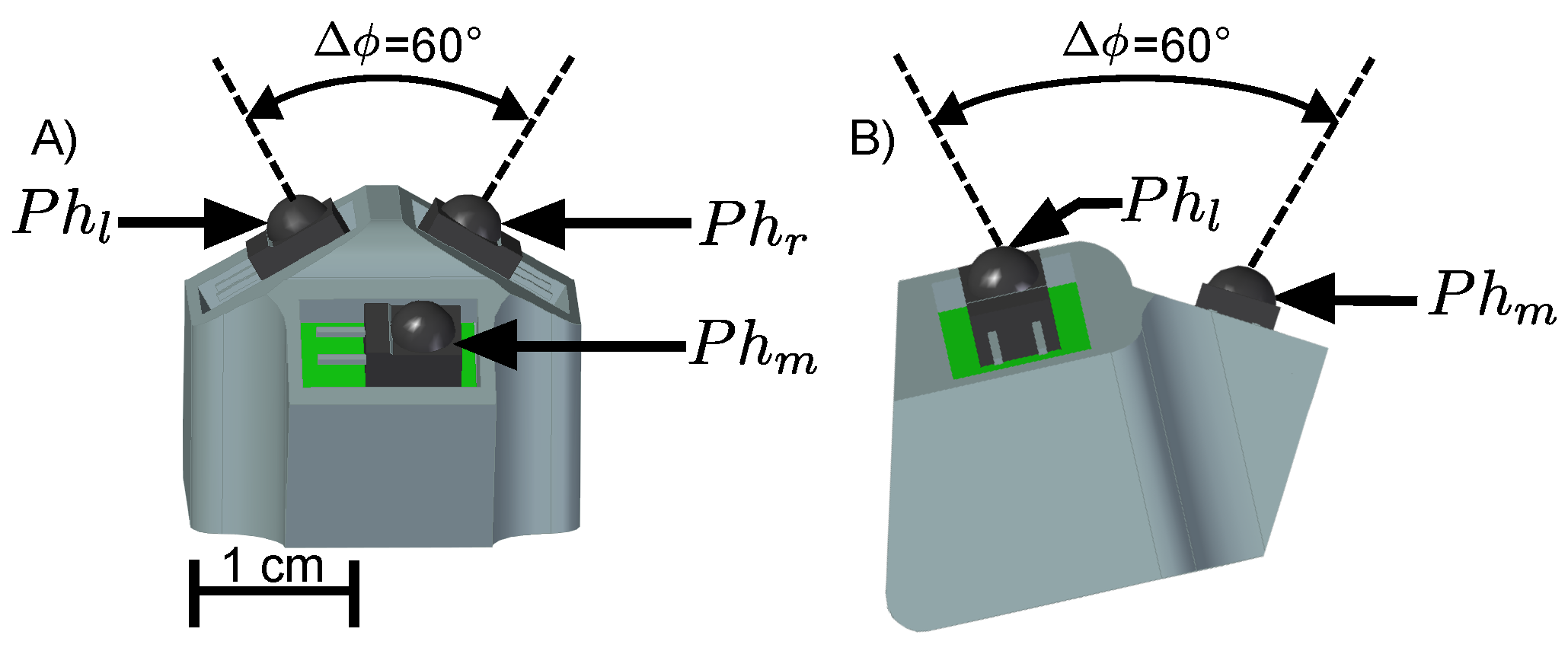
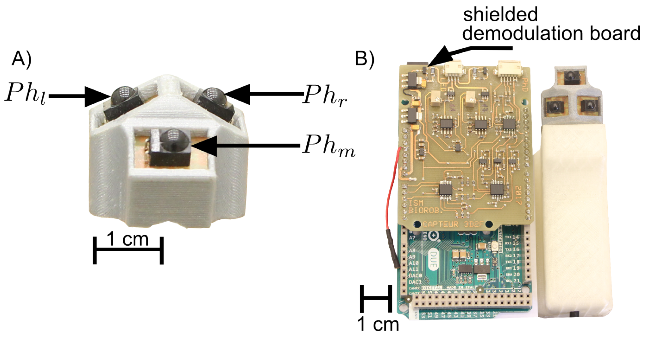
2. Sensor Design

The optical sensor device, called HyperCube, designed and developed in this study, is equipped with three photodiodes (Figure 1). Each photodiode is mounted on the face of a tetrahedron. As depicted in Figure 1A,B, the optical axis of each photodiode is separated by an inter-receptor angle $\Delta \varphi ={60}^{\circ }$, which defines the spatial acuity of the visual system [14].

3. Fabrication

The prototype of the sensor was obtained by 3D printing as shown on Figure 2A. It is equipped with three photodiodes made by Vishay Semiconductors with the reference BPV22F. Each photodiode has a maximum absorption at the wavelength of 950 nm which corresponds to the maximum emissive power of the infrared LEDs SF4249. As presented in Figure 2B, a custom-made electronic board for the frequency modulation of the flickering IR LEDs can produce two separate signals at 11 kHz and 17 kHz, respectively. The same electronic board composed of two analog demodulation circuits performs the acquisition and demodulation. Shielded on the Arduino board, the latter performs the visual signal processing and provides an estimation of the HyperCube’s angular position (i.e., azimuth and elevation angles) with respect to the infrared LEDs.

4. Modeling

Each photodiode features an angular sensitivity which is defined by the angle of acceptance denoted $\Delta \rho$, i.e., the full width at half maximum of the angular sensitivity. A bell-shaped sensitivity function models the angular sensitivity of each photodiode. It was inspired by the Gaussian angular sensitivity function of flies’ photoreceptors as described in [15].

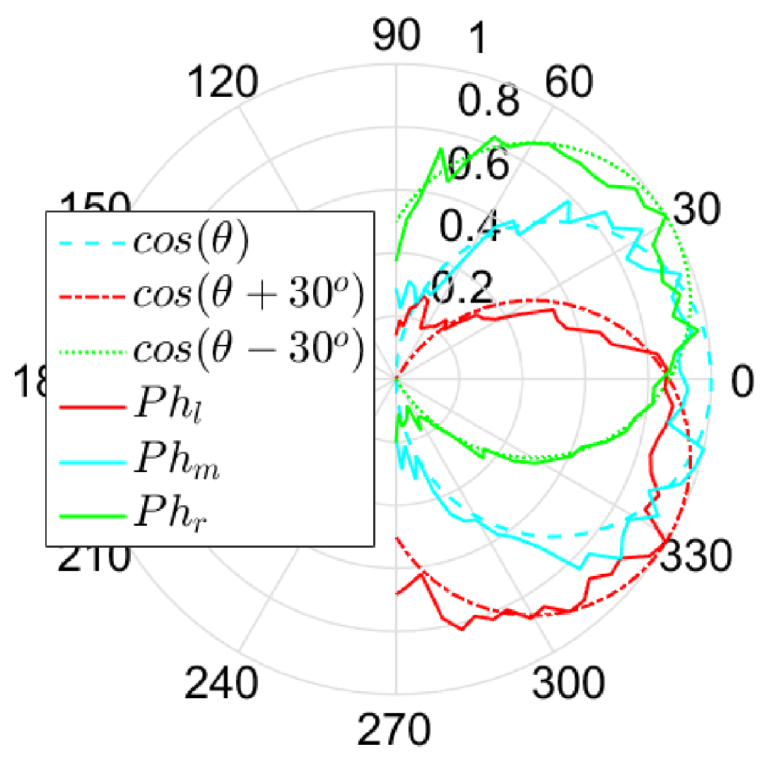
4.1. Angular Sensitivity of the Photosensors

As presented in Figure 3, the angular sensitivity of each photodiode in solid line is compared to the cosine-like angular sensitivity in dotted line. One can show that the cosine-like angular sensitivity of the model fits well to the experimental data and finally fits better than a Gaussian function. Moreover, the angle of acceptance $\Delta \rho$ is equal to ${120}^{\circ }$ and $\Delta \varphi$ between $P{h}_l$ and $P{h}_r$ is equal to ${60}^{\circ }$.

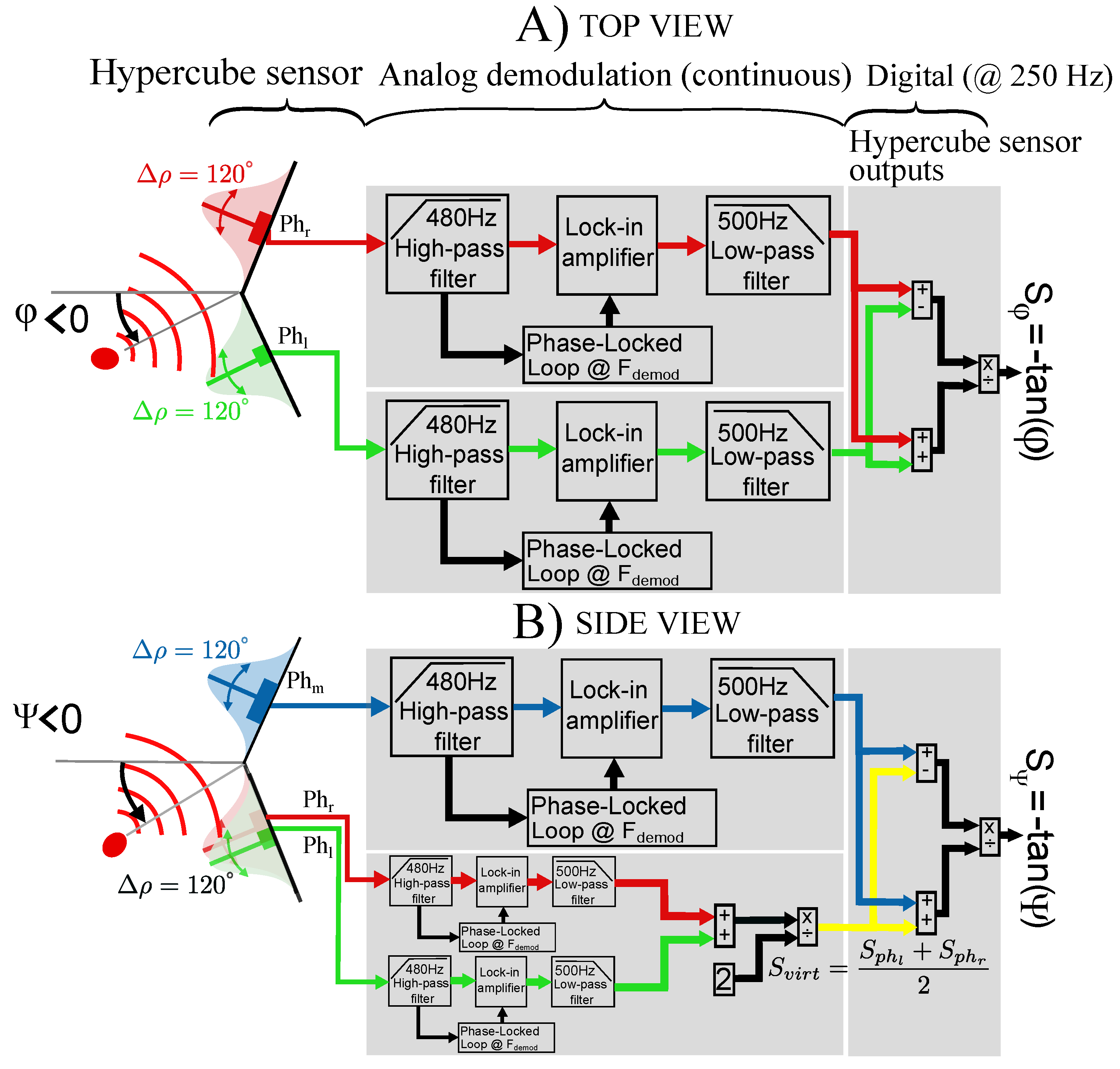
4.2. Principle of the Sensor

Two demodulated photodiode output signals are processed by an Arduino microcontroller. The analog demodulation steps were achieved by our custom-made shield board connected to the Arduino (see Figure 4). As shown in Figure 4A,B, the digital processing computes the relative difference over the sum of two adjacent demodulated photosensor output signals in order to assess the angular measurements (azimuth and elevation) [16]. The demodulation steps consist of using classical lock-in detection to demodulate the signal. However, the lock-in amplifier required a modulation signal which is provided here by a Phase-lock-loop circuit due to the fact that there is no physical link between the source (LED) and the receiver (photodiode).

As depicted in Figure 4, the digital processing operated in the microcontroller returns an output signal $S_{\phi }$ for the azimuth $\phi$ with $S_{\phi }=\frac{S_{p{h}_r}-S_{p{h}_l}}{S_{p{h}_r}+S_{p{h}_l}}$ and an output signal $S_{\psi }$ for the elevation $\psi$ with $S_{\psi }=\frac{S_{p{h}_m}-S_{p{h}_{virt}}}{S_{p{h}_m}+S_{p{h}_{virt}}}$ where $S_{virt}=\frac{S_{p{h}_l}+S_{p{h}_r}}{2}$. According to the visual sensor model mentioned in [13], $S_{\phi }\propto -tan\left(\phi \right)$ and $S_{\psi }\propto -tan\left(\psi \right)$. Therefore, the relative position $(\widehat{X},\widehat{Y})$ of the sensor with respect to the IR LED can be estimated with $\widehat{X}=-tan\left(\phi \right)\widehat{Z}$ and $\widehat{Y}\propto -tan\left(\psi \right)\widehat{Z}$, where $\widehat{Z}$ is the a priori known fixed height as shown on Figure 5.

5. Experimental Results

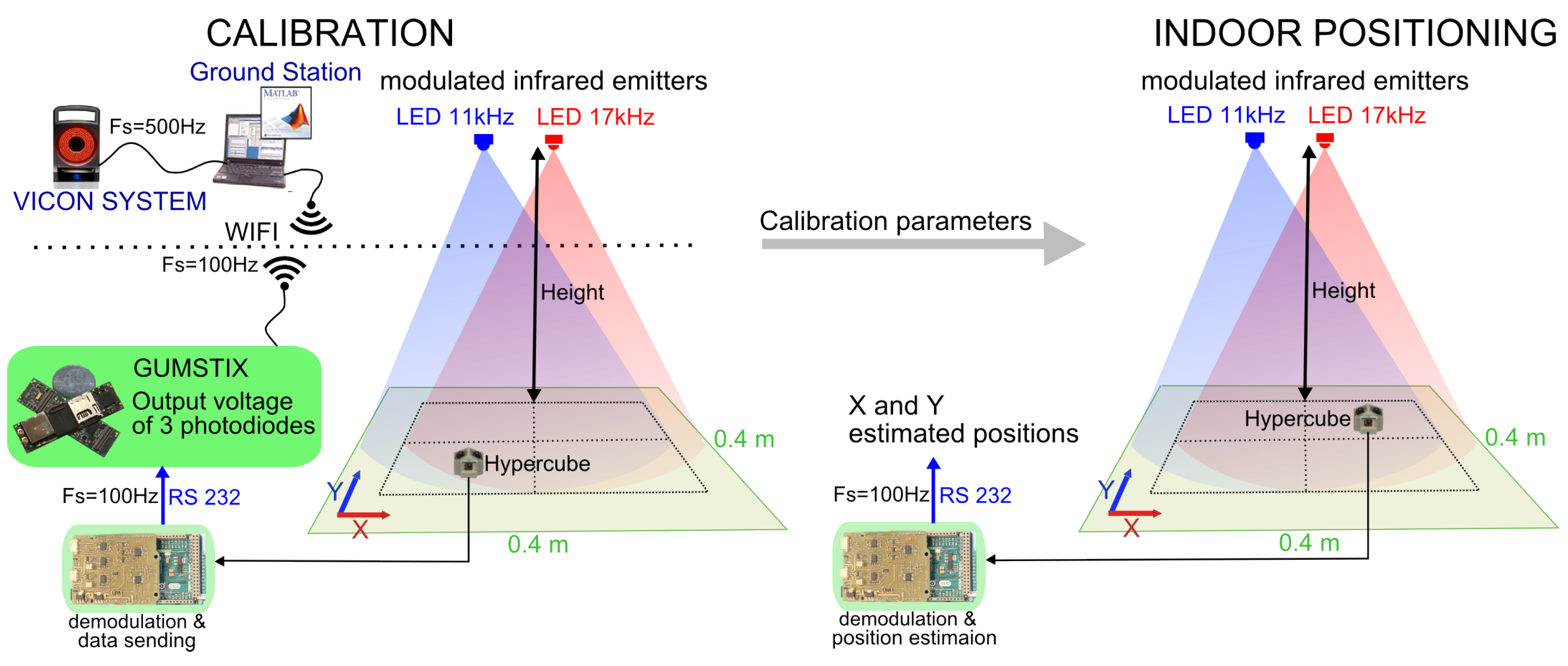
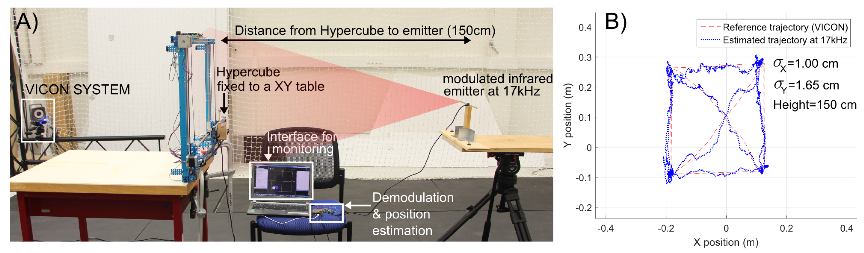
5.1. Position Estimation in 2D

A calibration, which consists of adjusting the sensor outputs $S_{\phi }$ and $S_{\psi }$ to the ratios $X/Z$ and $Y/Z$, is processed using the Vicon system.

$$\begin{array}{cc}\mathrm{minimize}\hfill & \frac{1}{n}\sum \sqrt{{(X_{ref}-\widehat{X})}^2+{(Y_{ref}-\widehat{Y})}^2}\hfill \\ \mathrm{subject}\mathrm{to}\hfill & -\frac{X_{ref}}{\widehat{Z}}=a_{\phi 1}.S_{\phi }^2+a_{\phi 2}.S_{\phi }+a_{\phi 3}.S_{\psi }^2+a_{\phi 4}.S_{\psi }+b_{\phi }\hfill \\ & -\frac{Y_{ref}}{\widehat{Z}}=a_{\psi 1}.S_{\phi }^2+a_{\psi 2}.S_{\phi }+a_{\psi 3}.S_{\psi }^2+a_{\psi 4}.S_{\psi }+b_{\psi }\hfill \end{array}$$

(1)

The coefficients $a_{\phi i}$ and $a_{\psi i}$ are determined using Matlab^®. The optimization Criterion (1) is to minimize the mean square error between the reference values and the actual data values provided by the sensor. The Matlab^® function fminunc is used to compute the coefficients. The localization was tested indoors for several lighting conditions. The optical sensing device was moving in X and Y at a fixed height as presented in Figure 5. After the calibration, the indoor localization is performed with the sole use of the optical sensor device connected to the demodulation board and the Arduino board.

Figure 6A gives a description of the experimental setup. One can see the location of the modulated infrared emitter and the coverage of the system. In this experiment, HyperCube is fixed to a XY table and moved by hand. One can note from the indoor localization results (Figure 6B) that the position estimation at the fixed height of 150 cm is accurate. The precision obtained features a standard deviation about 1 cm for X and inferior to 2 cm for Y measurements. Experiments over a longer distance are presented in the next section.

5.2. Localization of a Mobile Robot in 2D

In this section, we present the results obtained using HyperCube for indoor localizatin in 2D of a mobile robot. A new custom-made electronic board for the frequency modulation of the flickering IR LEDs is built. It can produce two separate signals at 5 kHz and 11 kHz. The mobile robot is equipped with a new custom-made electronic board composed of two analog demodulation circuits in charge of acquisition and demodulation. The experimental setup is presented in Figure 7. The ground height is $H=2$ m and the localization coverage area is 2 m × 2 m.

5.2.1. Kinematics and Dynamics Modeling of the Mobile Robot

Complete kinematics and dynamics modeling of the omni-directional robot with mecanum wheels are detailed in [17,18]. Figure 8 shows the disposition of the wheels related to the frames ${\mathrm{\Sigma }}_0$, ${\mathrm{\Sigma }}_{i\omega }$, (i = 1, 2, 3, 4). We define: $V_{i\omega }$ (i = 1, 2, 3, 4) the velocity vector corresponding to the wheels revolutions where $V_{i\omega }=R_w\times {\omega }_i$. $R_w$ is the radius of the wheel and ${\omega }_i$ is the revolution velocity of the wheel. $V_{ir}$ (i = 1, 2, 3, 4) is the tangential velocity vector of the free roller touching the floor and $V_0={\left[{\dot{x}}_m{\dot{y}}_m{\dot{\psi }}_m\right]}^T$ is the velocity vector in the local frame $(X_m,Y_m,Z_m)$.

The state vector $X={\left[xy\psi \right]}^T$ is composed of the positions x, y and the heading $\psi$ in the global frame $(X_G,Y_G,Z_G)$. Kinematics equation describing the relationship between $V_{\omega }$ and $V_0$ is given by:

$$V_{\omega }=J_0·V_0$$

(2)

$J_0=\left[\begin{array}{ccc}1& -1& -(l+L)\\ 1& 1& (l+L)\\ 1& 1& -(l+L)\\ 1& -1& (l+L)\end{array}\right]\in {\mathbb{R}}^{4\times 3}$ is a transformation matrix and $V_{\omega }={\left[V_{1\omega }{V}_{2\omega }{V}_{3\omega }{V}_{4\omega }\right]}^T$ is the wheel velocity vector corresponding to the angular velocity. Oppositely, the mobile robot velocity can be derived from the wheel velocity using a pseudo inverse matrix as in (3):

$$V_0={J_0}^{+}·V_{\omega }$$

(3)

where ${J_0}^{+}={\left({J_0}^T·J_0\right)}^{-1}{J_0}^T$. As a result, each element of $V_0$ is given by the following equations:

$${\dot{x}}_m=\frac{R_w}{4}\left({\omega }_1+{\omega }_2+{\omega }_3+{\omega }_4\right)$$

(4)

$${\dot{y}}_m=\frac{R_w}{4}\left(-{\omega }_1+{\omega }_2+{\omega }_3-{\omega }_4\right)$$

(5)

$${\dot{\psi }}_m=\frac{R_w}{4(L+l)}\left(-{\omega }_1+{\omega }_2-{\omega }_3+{\omega }_4\right)$$

(6)

The velocity $\dot{X}$ in the global frame $(X_G,Y_G,Z_G)$ is expressed in (7):

$$\left[\begin{array}{c}\dot{x}\\ \dot{y}\\ \dot{\psi }\end{array}\right]=\left[\begin{array}{ccc}cos\left(\psi \right)& -sin\left(\psi \right)& 0\\ sin\left(\psi \right)& cos\left(\psi \right)& 0\\ 0& 0& 1\end{array}\right]·\left[\begin{array}{c}{\dot{x}}_m\\ {\dot{y}}_m\\ {\dot{\psi }}_m\end{array}\right]$$

(7)

As presented in [18,19], the vehicle dynamics is given by (8):

$$\left[\begin{array}{c}\dot{\theta }\\ \ddot{\theta }\end{array}\right]=\left[\begin{array}{cc}{0}_{4\times 4}& I_{4\times 4}\\ 0_{4\times 4}& -M^{-1}{D}_{\theta }\end{array}\right]\left[\begin{array}{c}\theta \\ \dot{\theta }\end{array}\right]+\left[\begin{array}{c}{0}_{4\times 4}\\ M^{-1}\end{array}\right]\tau$$

(8)

$\theta ={\left[{\theta }_1{\theta }_2{\theta }_3{\theta }_4\right]}^T$ is the vector of the angular position of each wheel. $\tau ={\left[{\tau }_1{\tau }_2{\tau }_3{\tau }_4\right]}^T$ is the control input vector composed of the torque applied to each wheel with: $M=\left[\begin{array}{cccc}A+B+I_w& -B& B& A-B\\ -B& A+B+I_w& A-B& B\\ B& A-B& A+B+I_w& -B\\ A-B& B& -B& A+B+I_w\end{array}\right]$, $A=\frac{m{R_w}^2}{8}$, $B=\frac{I_z{R_w}^2}{16{(L+l)}^2}$ and $D_{\theta }$ is the coefficient of the wheel’s viscous friction. $I_z$ is the vehicle moment of inertia around the Z axis. $I_w$ is the wheel’s moment of inertia around the center of revolution.

5.2.2. Design of Position Control

The standard robot motion control have been designed using a sliding mode dynamic controller to track a desired trajectory as detailed in [19]. Let us consider the state vector $X={[x_{11},x_{12},x_{21},x_{22},x_{31},x_{32}]}^T={[\int x,x,\int y,y,\int \psi ,\psi ]}^T$ and the control input vector $u={\left[u_1{u}_2{u}_3\right]}^T={\left[{\dot{x}}_m{\dot{y}}_m{\dot{\psi }}_m\right]}^T$. From (7), the state space representation of the system is given by:

$$\begin{array}{cc}\hfill {\dot{x}}_{11}& =x_{12}\hfill \\ \hfill {\dot{x}}_{12}& =u_{1}cos\left(x_{32}\right)-u_{2}sin\left(x_{32}\right)\hfill \\ \hfill {\dot{x}}_{21}& =x_{22}\hfill \\ \hfill {\dot{x}}_{12}& =u_{1}sin\left(x_{32}\right)+u_{2}cos\left(x_{32}\right)\hfill \\ \hfill {\dot{x}}_{31}& =x_{32}\hfill \\ \hfill {\dot{x}}_{32}& =u_3\hfill \\ \hfill \end{array}$$

(9)

The control input vector $r={\left[r_1{r}_2{r}_3\right]}^T$ is defined to compensate for the nonlinear terms in (9)

$$\begin{array}{cc}\hfill u_1& =cos\left(x_{32}\right)r_1+sin\left(x_{32}\right)r_2\hfill \\ \hfill u_2& =-sin\left(x_{32}\right)r_1+cos\left(x_{32}\right)r_2\hfill \\ \hfill u_3& =r_3\hfill \\ \hfill \end{array}$$

(10)

Using (10) in the state space representation (9), a system of equations is written as following:

$$\begin{array}{c}\hfill {\sum }_1=\left\{\begin{array}{cc}{\dot{x}}_{11}\hfill & =x_{12}\hfill \\ {\dot{x}}_{12}\hfill & =r_1\hfill \end{array}\right.\end{array}$$

(11a)

$$\begin{array}{c}\hfill {\sum }_2=\left\{\begin{array}{cc}{\dot{x}}_{21}\hfill & =x_{22}\hfill \\ {\dot{x}}_{12}\hfill & =r_2\hfill \end{array}\right.\end{array}$$

(11b)

$$\begin{array}{c}\hfill {\sum }_3=\left\{\begin{array}{cc}{\dot{x}}_{31}\hfill & =x_{32}\hfill \\ {\dot{x}}_{32}\hfill & =r_3\hfill \end{array}\right.\end{array}$$

(11c)

The Equation (11a,b) stand for the equations of translation and the Equation (11c) describes the movement of rotation. As defined in [19], the positions of reference ${\xi }_{1d}$ and ${\xi }_{2d}$ in the inertial frame are introduced. The orientation reference in the same frame is also noted ${\xi }_{3d}$. Therefore, the following subsystem of equations is written:

$$\begin{array}{c}\hfill {\sum }_i^e=\left\{\begin{array}{cc}{\dot{z}}_{i1}\hfill & =z_{i2}\hfill \\ {\dot{z}}_{i2}\hfill & =r_i-{\dot{\xi }}_{id}\forall i\in \{1,2,3\}\hfill \\ {\dot{\varphi }}_{id}\hfill & ={\xi }_{id}\hfill \end{array}\right.\end{array}$$

(12a)

with $z_{i1}=x_{i1}-{\varphi }_{id}$, $z_{i2}=x_{i2}-{\xi }_{id}\forall i\in \{1,2,3\}$. The saturation function denoted ${\sigma }_M:\mathbb{R}\to \mathbb{R}$ is defined as:

$$\begin{array}{c}\hfill {\sigma }_M\left(S\right)=\left\{\begin{array}{c}Sif\left|S\right|<M\hfill \\ sign\left(S\right)\times Motherwise\hfill \end{array}\right.\end{array}$$

(13a)

The sliding surfaces $S_{i1}$ and $S_{i2}$ are defined for each axis X and Y such that:

$$\begin{array}{cc}\hfill S_{i1}& =a_{i1}{a}_{i2}{z}_{i1}-a_{i2}{z}_{i2}\hfill \\ \hfill S_{i2}& =a_{i1}{z}_{i2}\hfill \end{array}$$

(14)

where the coefficients $a_{i1}$ and $a_{i2}$ are chosen to ensure the attractiveness of the sliding surfaces. Therefore, we propose the candidate Lyapunov functions $V_{i1}$ and $V_{i2}$ for each sliding surface:

$$\begin{array}{cc}\hfill V_{i1}& =S_{i1}^2\hfill \\ \hfill V_{i2}& =S_{i2}^2\hfill \end{array}$$

(15)

As explained in [19], the exponential stability of the system is ensured and the control input signal $r_i$ can be written as:

$$\begin{array}{c}\hfill r_i={\sigma }_{i3}({\dot{\xi }}_{id}-{\sigma }_{M_{i2}}(a_{i1}{z}_{i2}+{\sigma }_{M_{i1}}(a_{i2}{z}_{i2}+a_{i1}{a}_{i2}{z}_{i1})))\forall i\in \{1,2,3\}.\end{array}$$

(16)

Using (10) and the expression provided by (16), the control input signals $u_1$, $u_2$ and $u_3$ are bounded such as:

$$\begin{array}{cc}\hfill |u_1|& =max(M_{13},M_{23},0.707(M_{13}+M_{23}))\hfill \\ \hfill |u_2|& =max(M_{13},M_{23},0.707(M_{13}+M_{23}))\hfill \\ \hfill |u_3|& =M_{33}\hfill \end{array}$$

(17)

Therefore, the angular speed of each wheel ${\omega }_i$ of the mobile robot is bounded such as the following:

$$\begin{array}{cc}\hfill |{\omega }_1|& =\frac{1}{R_w}\left((L+l)M_{33}\right)\hfill \\ \hfill |{\omega }_2|& =\frac{1}{R_w}(2·max(M_{13},M_{23},0.707(M_{13}+M_{23}))+(L+l)M_{33})\hfill \\ \hfill |{\omega }_3|& =\frac{1}{R_w}(2·max(M_{13},M_{23},0.707(M_{13}+M_{23}))+(L+l)M_{33})\hfill \\ \hfill |{\omega }_4|& =\frac{1}{R_w}\left((L+l)M_{33}\right)\hfill \end{array}$$

(18)

where $M_{ij},\forall i,j\in \{1,2,3\}$ is the saturation parameter as defined in (13a). Figure 9 presents the block diagram of the system. The position and heading of the mobile robot are controlled in closed loop. It is worth noting that:

• The nonlinear control block computes each angular reference speed ${\omega }_i^{*}$ for the wheel i. The control law minimizes the error between the reference position $X^{*}$ and the position estimate $\widehat{X}$.
• The angular speed of each wheel is controlled in closed loop using a local proportional integral controller (PI).
• The estimated position and heading of the mobile robot collected in the vector $\widehat{X}=(\widehat{x},\widehat{y},\widehat{\varphi })$ are provided by HyperCube or the Vicon motion capture system .

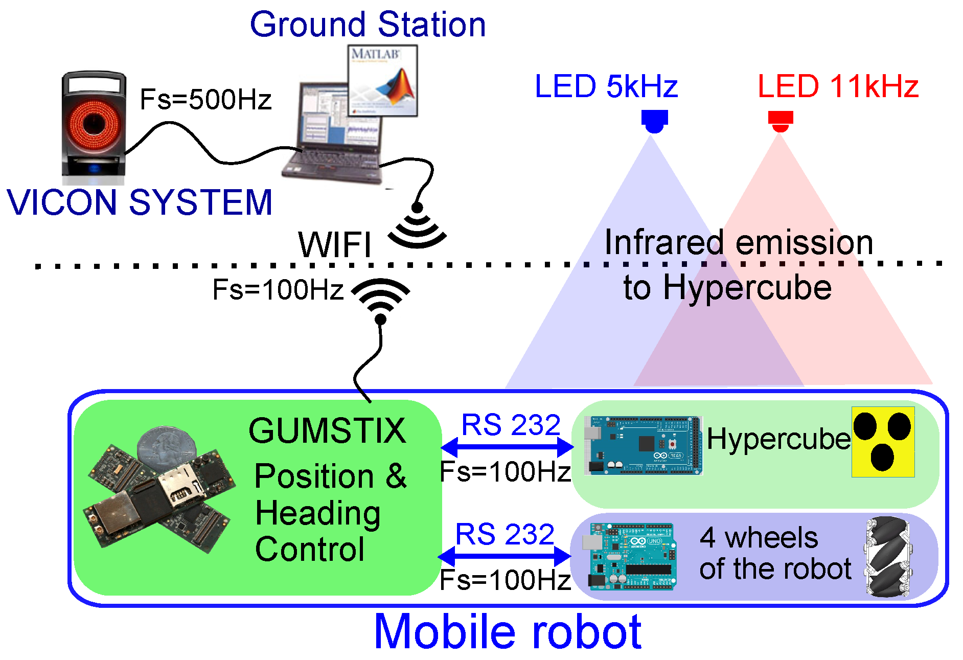
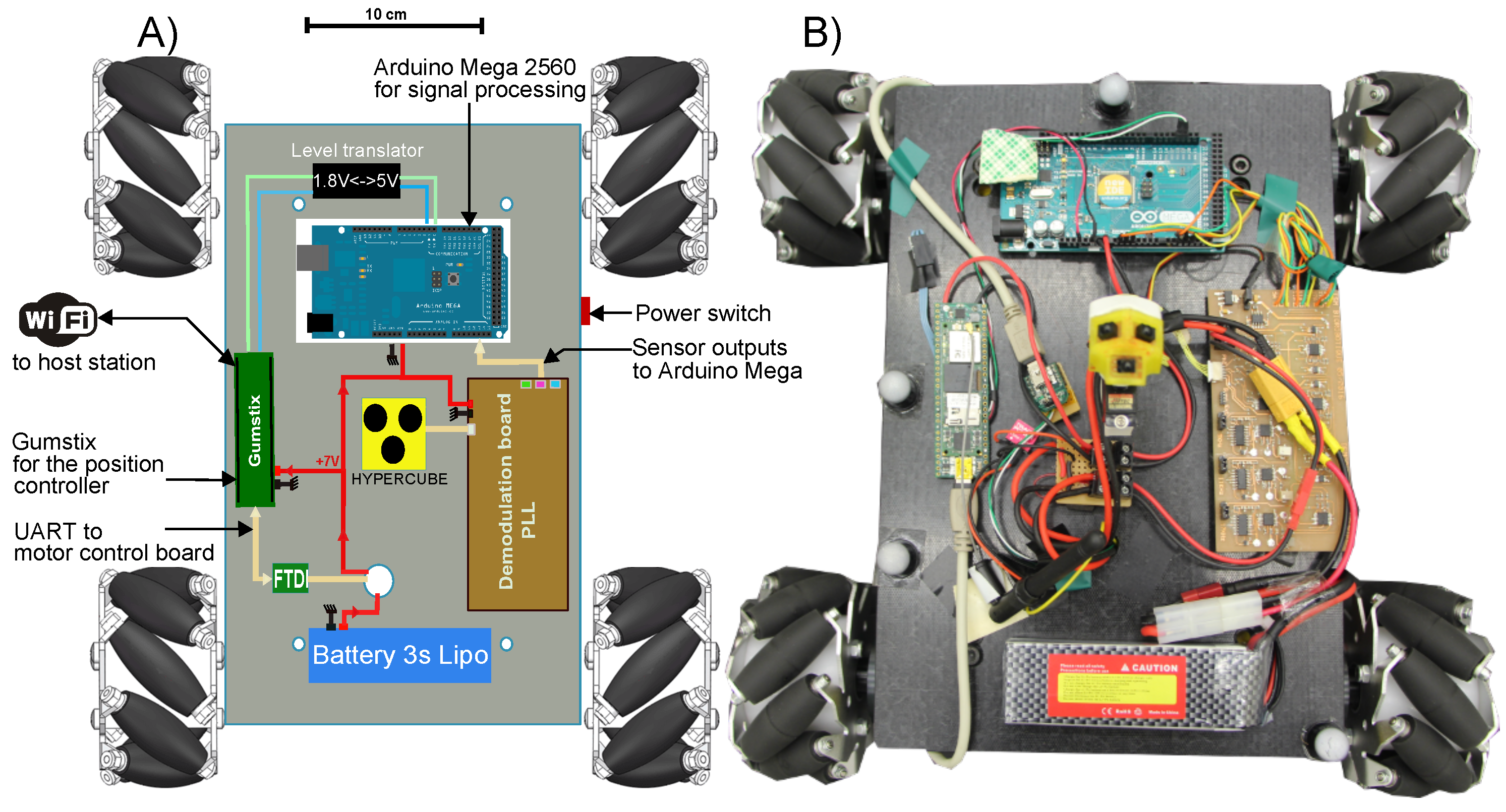
5.2.3. Implementation of the Indoor Localization for the Mobile Robot

To evaluate the performances of the indoor localization, the setup detailed in Figure 10 is composed of the following:

• The Vicon motion capture system featuring sub-millimetric accuracy. It provides the localization estimation of the mobile robot. The motion capture data are used for comparison purposes.
• The ground station connected to the Vicon system runs Matlab/Simulink^® and QUARC^® software programs. The nonlinear control law of the mobile robot presented in Section 5.2.2 is designed with Matlab/Simulink^® and compiled. The program is transferred via WIFI radio link to the Gumstix microcontroller embedded on the mobile robot. The control algorithm runs onboard the robot.

The mobile robot aims at tracking a desired trajectory using HyperCube in a feedback control loop. An Arduino 380 board controls in closed-loop the angular velocity of each wheel. An Arduino Mega 2560 board is connected to the custom-made demodulation board of HyperCube which provides analog signals. The analog processing of the photodiode’s output signal is depicted in Figure 4. The Gumstix board uses the estimation of the robot position $\widehat{X}=(\widehat{x},\widehat{y},\widehat{\varphi })$ for control purpose.

Figure 11A gives a schematic of the hardware embedded on the mobile robot for indoor localization using HyperCube. Figure 11B shows the hardware implementation and HyperCube mounted onboard the mecanum wheeled omni-directional robot. Four reflective markers make the mobile robot visible by the Vicon system.

5.2.4. Application to the 2D Localization

The aim of this section is twofold: (i) using HyperCube in open loop, reconstruct the trajectory $(x,y)$ of the mobile robot in the coverage area presented in Figure 7; and (ii) using HyperCube in closed loop, track a desired trajectory. For that purpose, the following experiments are performed.

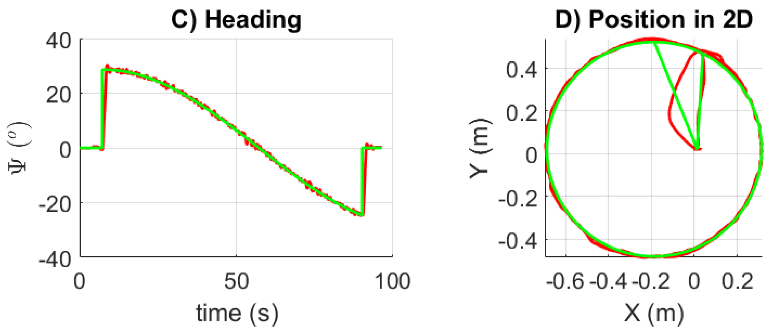
5.2.5. Validation of the Nonlinear Control Law for Trajectory Tracking

The Vicon cameras provide to the nonlinear controller detailed in Section 5.2.2 the accurate localization and orientation of the robot in real-time. The mobile robot moves on a circular path of diameter 1 m. In the same time, the desired orientation $\psi$ is a sinus. The results are given in Figure 12 where Figure 12A–C shows in red the positions $(x,y)$ and the heading $\psi$ versus time of the mobile robot compared to the reference in green. Figure 12D plots y versus x. Using accurate estimations of position and heading, the mobile robot follows the desired trajectory with precision without overshoot. This result validates the good performances of the sliding mode nonlinear control law.

5.2.6. Trajectory Reconstruction Using HyperCube

While keeping the circular path of diameter 1 m as reference, the desired orientation $\psi$ is regulated at zero. The mecanum wheeled omni-directional robot maintains its orientation along the path. In this experiment, the trajectory is reconstructed using the measurements provided by HyperCube and only one IR LED that flickers at 11 kHz. However, the estimated positions provided by HyperCube were not used to control in closed-loop the robot. Figure 13 shows the results of the reconstruction. In Figure 13A,B, the position estimations in X and Y are plotted versus time and compared to the ground truth provided by the Vicon system. Figure 13C presents the heading $\psi$ which is maintained at zero. There is no curve for HyperCube since HyperCube is not used to estimate the heading. Figure 13D depicts the XY graph. Satisfactory trajectory reconstruction can be verified by comparing the actual path of the mobile robot to the estimated one given by HyperCube.

One can see in Figure 14A,B the plots of the autocorrelation functions of the residuals. The noise for each axis has nearly white characteristics.

Moreover, given $H=2$ m, the precision obtained reaches a standard deviation as small as $1.86$ cm for X and $1.37$ cm for Y (see Figure 15). Looking accross the precision of the reconstruction, the mobile robot was then controlled by means of HyperCube.

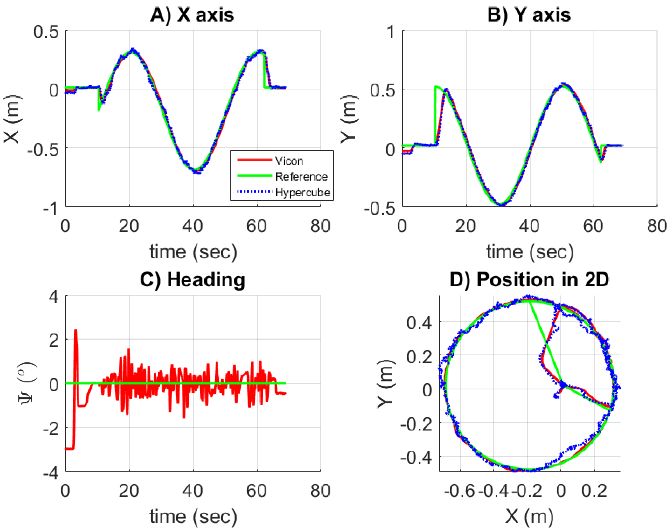
5.2.7. Robot Closed-Loop Control Based on HyperCube

In this section, the goal was to use the measurements provided by HyperCube to control in closed-loop the linear positions (x, y) of the robot. The current version of the sensor can only estimate the positions but not the rotations. For a robotic application using aerial robots for instance, HyperCube could be associated to a stabilizing gimbal system to reduce the effects of the variations of roll and picth angles which could affect the measurements. In the present application, the orientation $\psi$ is given by the Vicon cameras. If we denote $x_{sensor}$ and $y_{sensor}$ the coordinates of the mobile robot in the local frame, the estimates of position $\widehat{x}$ and $\widehat{y}$ in the global frame are obtained by applying the rotation matrix as following:

$$\left[\begin{array}{c}\widehat{x}\\ \widehat{y}\\ \widehat{\psi }\end{array}\right]=\left[\begin{array}{ccc}cos\left(\widehat{\psi }\right)& -sin\left(\widehat{\psi }\right)& 0\\ sin\left(\widehat{\psi }\right)& cos\left(\widehat{\psi }\right)& 0\\ 0& 0& 1\end{array}\right]\left[\begin{array}{c}{x}_{sensor}\\ y_{sensor}\\ {\psi }_{vicon}\end{array}\right]$$

(19)

where ${\psi }_{vicon}$ is the estimation of the orientation given by the Vicon cameras. Figure 16 shows the results while the sensor is used in closed loop. The orientation $\psi$ is estimated with the motion capture system. Figure 16A,B superimposes the positions x and y measured by HyperCube (blue curve) and by the Vicon system (red curve). Figure 16C presents the regulation of the heading versus time. Since the orientation is given by the Vicon cameras and not by HyperCube, there is no curve related to HyperCube in Figure 16C. Once equipped with HyperCube, the experimental results show that HyperCube can be suitable to make the mobile robot follow faithfully the reference trajectory. Therefore, the performance of the HyperCube sensor have been validated indoors by using only one flickering IR LED. A limitation of this solution is the need of the orientation $\psi$ provided by the Vicon system. However, for this kind of application, onboard sensors such as a low-cost inertial measurement unit (IMU) for instance in [20], magnetometer as proposed in [21] or odometry could be used to get the heading in real time.

6. Conclusions

In this paper, we proposed a novel positioning system for indoor application which can measure the angular position of a moving optical sensor, HyperCube. The latter was coupled to an Arduino-compatible demodulator through a custom-made shield board. Based on infrared light emission, the proposed solution for indoor localization spotlights the following features: (i) a minimalistic sensor in terms of small size (10 cm${}^3$), light weight (6 g) and low power consumption (0.4 W for the sensor and the analog demodulation board); (ii) a fast analog signal processing and a digital processing implemented on an Arduino microcontroller (difference over the sum); and (iii) an online accurate position estimation in 2D.

We have shown that the proposed sensor was able to estimate the position in 2D at a distance of 1.5 m from the LEDs with an accuracy as small as 1-cm at a sampling frequency of 100 Hz using only one IR LED flickering at 17 kHz. We also proposed a robotic application which consisted in localizing a moving mecanum wheeled omnidirectional robot indoors. For a trajectory reconstruction purpose, the precision of the position estimation reached good performances with a standard deviation as small as 1.86 cm for X and 1.37 cm for Y with only one flickering IR LED placed at 2 m above the robot. To show the performance of HyperCube, the sensor was implemented in the position feedback control loop to make the mobile robot able to track a reference trajectory (a circle of 1 m in diameter). It turned out that the mobile robot followed the desired path faithfully, validating that the indoor local positioning system using flickering IR LEDs is a reliable and an efficient solution.

To further improve the performance of the proposed system, the sensor measurements provided by HyperCube will be fused with other sensors such as IMU to improve the position estimation. The height could also be estimated using two IR LEDs at two different frequencies. Moreover, one could investigate the estimation of the heading $\psi$ using several IR LEDs at the same time.

References

- Bahl, P.; Padmanabhan, V.N. RADAR: An in-building RF-based user location and tracking system. In Proceedings of the INFOCOM 2000 Nineteenth Annual Joint Conference of the IEEE Computer and Communications Societies, Tel Aviv, Israel, 26–30 March 2000; Volume 2, pp. 775–784. [Google Scholar]
- Raja, A.K.; Pang, Z. High accuracy indoor localization for robot-based fine-grain inspection of smart buildings. In Proceedings of the 2016 IEEE International Conference on Industrial Technology (ICIT), Taipei, Taiwan, 14–17 March 2016; pp. 2010–2015. [Google Scholar]
- Kjærgaard, M.B. A taxonomy for radio location fingerprinting. In Proceedings of the International Symposium on Location-and Context-Awareness, Oberpfaffenhofen, Germany, 20–21 September 2007; Springer: Berlin, Germany, 2007; pp. 139–156. [Google Scholar]
- Reinke, C.; Beinschob, P. Strategies for contour-based self-localization in large-scale modern warehouses. In Proceedings of the 2013 IEEE 9th International Conference on Intelligent Computer Communication and Processing (ICCP), Cluj-Napoca, Romania, 5–7 September 2013; pp. 223–227. [Google Scholar]
- Scaramuzza, D.; Fraundorfer, F. Visual Odometry [Tutorial]. IEEE Robot. Autom. Mag. 2011, 18, 80–92. [Google Scholar] [CrossRef]
- Frassl, M.; Angermann, M.; Lichtenstern, M.; Robertson, P.; Julian, B.J.; Doniec, M. Magnetic maps of indoor environments for precise localization of legged and non-legged locomotion. In Proceedings of the 2013 IEEE/RSJ International Conference on Intelligent Robots and Systems, Tokyo, Japan, 3–7 November 2013; pp. 913–920. [Google Scholar]
- Yasir, M.; Ho, S.W.; Vellambi, B.N. Indoor Position Tracking Using Multiple Optical Receivers. J. Lightw. Technol. 2016, 34, 1166–1176. [Google Scholar] [CrossRef]
- Sakai, N.; Zempo, K.; Mizutani, K.; Wakatsuki, N. Linear Positioning System based on IR Beacon and Angular Detection Photodiode Array. In Proceedings of the International Conference on Indoor Positioning and Indoor Navigation (IPIN), Alcalá de Henares, Spain, 4–7 October 2016; pp. 4–7. [Google Scholar]
- Simon, G.; Zachár, G.; Vakulya, G. Lookup: Robust and Accurate Indoor Localization Using Visible Light Communication. IEEE Trans. Instrum. Meas. 2017, 66, 2337–2348. [Google Scholar] [CrossRef]
- Arnon, S. Visible Light Communication; Cambridge University Press: Cambridge, UK, 2015. [Google Scholar]
- Komine, T.; Nakagawa, M. Fundamental analysis for visible-light communication system using LED lights. IEEE Trans. Consum. Electron. 2004, 50, 100–107. [Google Scholar] [CrossRef]
- Ijaz, F.; Yang, H.K.; Ahmad, A.; Lee, C. Indoor positioning: A review of indoor ultrasonic positioning systems. In Proceedings of the 2013 15th International Conference on Advanced Communication Technology (ICACT), PyeongChang, Korea, 27–30 January 2013; pp. 1146–1150. [Google Scholar]
- Raharijaona, T.; Mignon, P.; Juston, R.; Kerhuel, L.; Viollet, S. HyperCube: A Small Lensless Position Sensing Device for the Tracking of Flickering Infrared LEDs. Sensors 2015, 15, 16484–16502. [Google Scholar] [CrossRef] [PubMed]
- Land, M.F. Visual acuity in insects. Annu. Rev. Entomol. 1997, 42, 147–177. [Google Scholar] [CrossRef] [PubMed]
- Stavenga, D. Angular and spectral sensitivity of fly photoreceptors. II. Dependence on facet lens F-number and rhabdomere type in Drosophila. J. Comp. Physiol. A 2003, 189, 189–202. [Google Scholar]
- Kerhuel, L.; Viollet, S.; Franceschini, N. The VODKA Sensor: A Bio-Inspired Hyperacute Optical Position Sensing Device. IEEE Sens. J. 2012, 12, 315–324. [Google Scholar] [CrossRef]
- Viboonchaicheep, P.; Shimada, A.; Kosaka, Y. Position rectification control for Mecanum wheeled omni-directional vehicles. In Proceedings of the IECON’03 29th Annual Conference of the IEEE Industrial Electronics Society, Roanoke, VA, USA, 2–6 November 2003; IEEE: Piscataway, NJ, USA, 2003; Volume 1, pp. 854–859. [Google Scholar]
- Lin, L.C.; Shih, H.Y. Modeling and adaptive control of an omni-mecanum-wheeled robot. Intell. Control Autom. 2013, 4, 166–179. [Google Scholar] [CrossRef]
- Guerrero-Castellanos, J.; Villarreal-Cervantes, M.; Sanchez-Santana, J.; Ramirez-Martinez, S. Seguimiento de trayectorias de un robot movil (3,0) mediante control acotado. Revista Iberoamericana de Automática e Informática Industrial RIAI 2014, 11, 426–434. [Google Scholar] [CrossRef]
- Euston, M.; Coote, P.; Mahony, R.; Kim, J.; Hamel, T. A complementary filter for attitude estimation of a fixed-wing UAV. In Proceedings of the IROS 2008 IEEE/RSJ International Conference on Intelligent Robots and Systems, Nice, France, 22–26 September 2008; IEEE: Piscataway, NJ, USA, 2008; pp. 340–345. [Google Scholar]
- Kim, H.S.; Seo, W.; Baek, K.R. Indoor Positioning System Using Magnetic Field Map Navigation and an Encoder System. Sensors 2017, 17, 651. [Google Scholar] [CrossRef] [PubMed]
© 2017 by the authors. Licensee MDPI, Basel, Switzerland. This article is an open access article distributed under the terms and conditions of the Creative Commons Attribution (CC BY) license (http://creativecommons.org/licenses/by/4.0/).
Share and Cite
Raharijaona, T.; Mawonou, R.; Nguyen, T.V.; Colonnier, F.; Boyron, M.; Diperi, J.; Viollet, S. Local Positioning System Using Flickering Infrared LEDs. Sensors 2017, 17, 2518. https://doi.org/10.3390/s17112518
Raharijaona T, Mawonou R, Nguyen TV, Colonnier F, Boyron M, Diperi J, Viollet S. Local Positioning System Using Flickering Infrared LEDs. Sensors. 2017; 17(11):2518. https://doi.org/10.3390/s17112518
Chicago/Turabian StyleRaharijaona, Thibaut, Rodolphe Mawonou, Thanh Vu Nguyen, Fabien Colonnier, Marc Boyron, Julien Diperi, and Stéphane Viollet. 2017. "Local Positioning System Using Flickering Infrared LEDs" Sensors 17, no. 11: 2518. https://doi.org/10.3390/s17112518
APA StyleRaharijaona, T., Mawonou, R., Nguyen, T. V., Colonnier, F., Boyron, M., Diperi, J., & Viollet, S. (2017). Local Positioning System Using Flickering Infrared LEDs. Sensors, 17(11), 2518. https://doi.org/10.3390/s17112518