1. Introduction
Due to the enormous progress in availability and performance of laser light sources and electro-optical components, tunable diode laser absorption spectroscopy (TDLAS) has entered various disciplines both in research and industrial applications. Being a highly-sensitive, selective, fast, non-destructive and in situ method, TDLAS is currently more and more used for quantitative assessment of gas concentration in several fields. These include, to mention only a few, atmospheric environmental monitoring [
1,
2,
3,
4,
5,
6], medical diagnostics [
7,
8,
9], chemical analysis [
10], and industrial process control [
11,
12,
13]. The increasing number of applications has pushed the requirements for this method both in terms of sensitivity and in terms of stability. On the other hand, for practical and commercial applications, there is a growing interest in compact, simple in design and cost-effective sensitive sensors that do not require special optical components but guarantee the sensitivity achievable with complex laboratory equipment.
One of the most common limits to the sensor performance is the presence of unwanted interference fringes due to etalons [
14]. These interferences may arise due to multiple reflections from reflecting or scattering surfaces in the system, like mirrors, lenses, optical fiber end faces, laser-head windows or dust particles in the gas [
14]. Even surfaces that are diffusive, for example due to dust deposited on sensor windows, can give rise to fringes over time [
15]. In particular, fringes that have a free spectral range (FSR) on the order of the width of the absorption lines contribute to significant errors in the determination of the line features. Special strategies have been proposed to deal with these types of interferences, as, for example, in [
16], where for small fringe amplitudes and a measurement window that is a multiple of the fringe FSR, the fringe was removed by an analysis in the Fourier domain. Furthermore, since the amplitude and the frequency of these interferences depend on the distance and alignment of the optical elements, they are affected by temperature changes and by mechanical disturbances, giving rise, for example, to a drift of the output signal, thus worsening the long-term performance of the system [
17].
The simplest strategy to reduce the effects of interference fringes consists of using anti-reflection coating and wedging or angling of the optical surfaces. Other approaches include, to mention only few, dithering one of the surfaces creating the interference and integrating the signal so as to average out its influence [
18,
19], selecting a particular modulation frequency [
20] or modulation scheme [
21,
22], specifically choosing the distance between the interfering surfaces [
23], and post-processing filtering [
24]. A comprehensive review on signal enhancement and noise reduction techniques can be found in [
25]. Although all of these approaches have been successfully implemented in past years, they nonetheless have limitations in the practical implementation depending on the application-specific conditions. For example, it may not always be possible to dither one surface, and the application of a specific detection scheme may limit the flexibility of the measurement.
In this work, a new and widely usable approach is presented that relies only on post processing of the data. Therefore, it requires no modification to the apparatus setup or hardware, and can be easily adapted to different experimental configurations. The new presented algorithm allows the extraction of a signal, as the absorption lines of a gas molecule, from a background containing arbitrary disturbances without having to make any assumption on the characteristics of these disturbances in terms of functional form. Therefore, it has the potential to improve the sensitivity and the stability of TDLAS. Furthermore, this algorithm, which is particularly easy to implement if the Fourier transform of the signal can be written in closed form, is very general and can be applied to any kind of spectroscopic data. The paper is organized as follows:
Section 2 describes the fundamentals of the method and of the algorithm;
Section 3 demonstrates its application to simulated signals; and
Section 4 shows the results for a case of direct absorption spectroscopy for oxygen gas sensing.
2. Description of the Algorithm
The algorithm described in this work has the ability to identify a spectroscopic feature from an arbitrary background that does not need to be modeled. The total signal detected in an experiment, here referred to as “total signal”
, is modeled as a sum of two contributions: one spectroscopic feature, like an absorption line, referred to here as “signal”
and a background referred to here as “background”
:
In the case of direct absorption spectroscopy,
is the absorbance and
is the distorted absorbance due to
. As mentioned above, the method shines if the background
cannot be modeled by a known analytical expression. In fact, if
is not known, it is not possible to perform a nonlinear fit of
and extract the signal
without making assumptions on the functional form of
. On the other hand, if the functional form is known but very complex, the algorithm may be advantageous because the inclusion of the background in the nonlinear fit may not be possible. Another significant advantage of the proposed algorithm is that the extraction works equally well independently of the amplitude of the interferences, as it will be shown in
Section 3 and
Section 4.
2.1. Steps of the Algorithm: General Description
Before describing the steps of the algorithm, the nomenclature and hypothesis for its applicability are introduced. The algorithm is based on the main hypothesis that the Fourier transform of the background
is significantly different than zero only for values of
k smaller than a certain cut-off
where
denotes the continuous Fourier transform (CFT),
a cut-off frequency and
contains the contribution of
for
, which is assumed to be negligible. One central aspect is the determination of a reasonable estimate for this cut-off frequency, as described in the section “Determine the cut-off frequency”.
Note that this formulation applies to continuous functions. Since in practice there will always be only a discrete set of points, it is necessary to approximate the CFT in Equation (
2) by a modified discrete Fourier transform (DFT)
where
denotes the modified DFT defined in
Appendix A Equation (
A6),
the cut-off point corresponding to the cut-off frequency
, and
contains the contribution of
for
, which is assumed to be negligible.
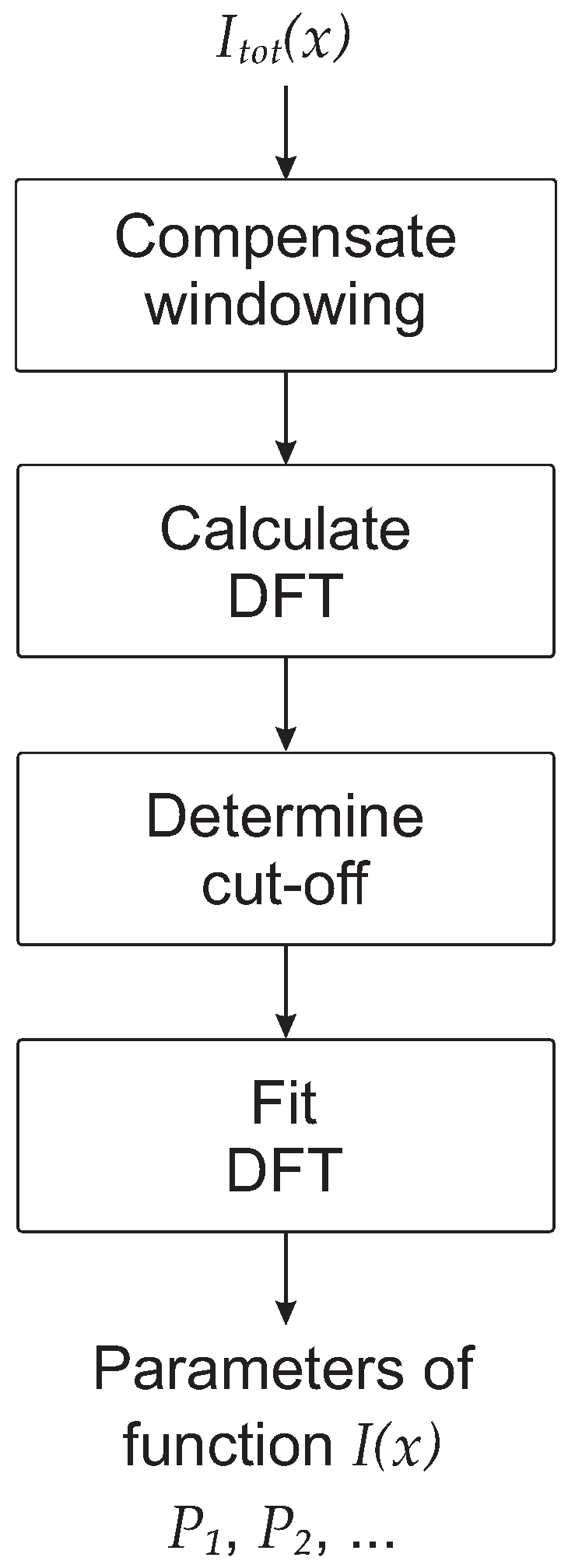
The schematic flow diagram of the algorithm is shown in
Figure 1 to give the reader a high-level understanding of the idea behind it. The single steps are described in detail below.
2.2. Compensate Windowing
In all experiments, the data always cover a limited range in the
x-direction. For example, the data shown in this paper are measured for a finite laser wavelength range. Mathematically, this is equivalent to applying a rectangular window (RW) before calculating the Fourier transform. This is a problem that, if not addressed, will limit the precision that can be achieved with the described algorithm. In fact, the RW results in making
in Equation (
2) not negligible anymore, and thus leads to an error in the fitting procedure of
. This is due to the fact that the DFT of a RW has an amplitude envelope that is proportional to
, and so it does not go to zero fast enough [
26].
To reduce the effect of windowing considerably, the proposed algorithm applies a more intelligent window. The not so often used Tukey window [
27,
28] has remarkable properties that help tremendously in reducing
dramatically. The Tukey window, indicated with
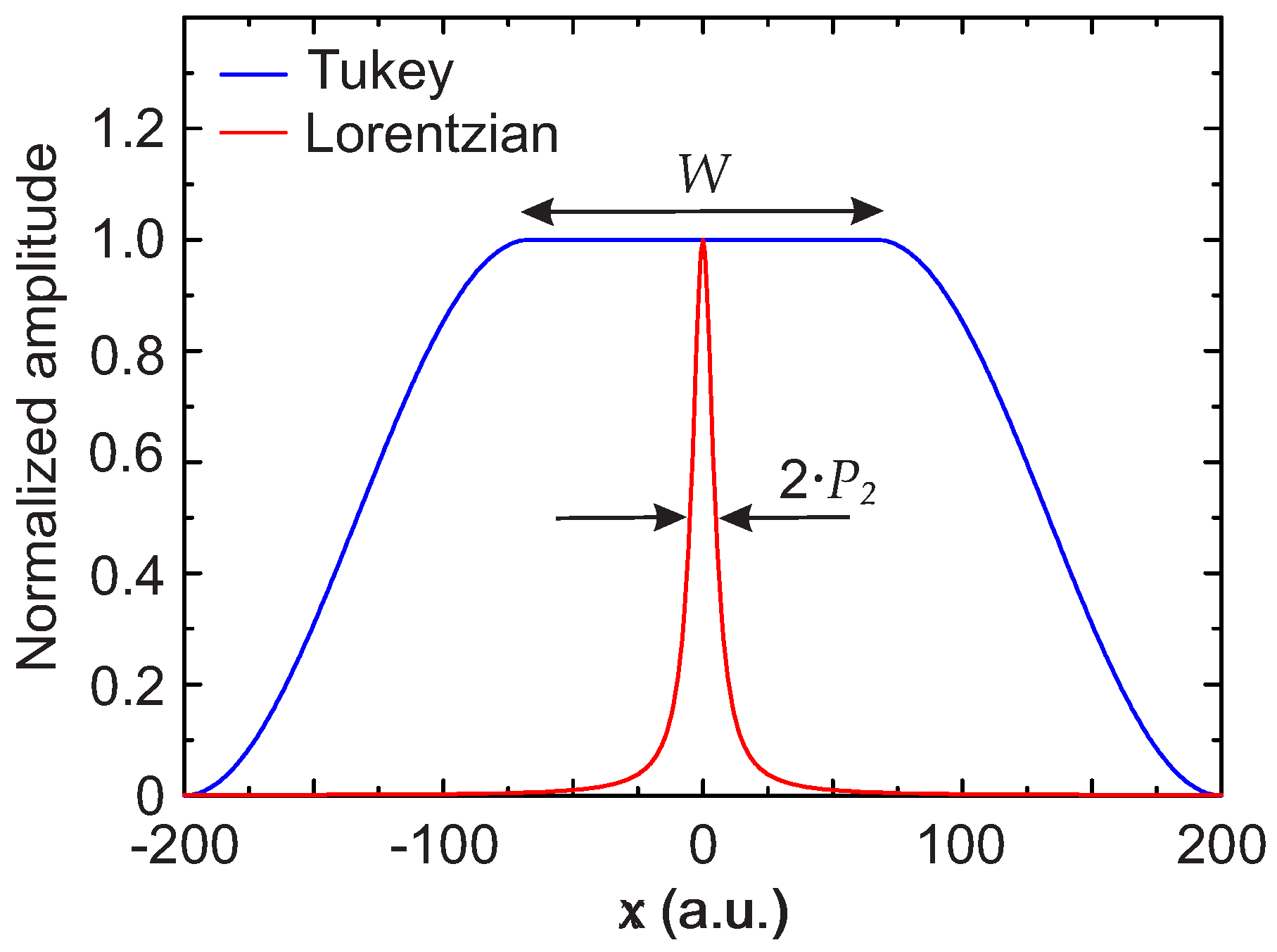
, is a perfectly flat (constant) symmetric function in the middle that then decreases rapidly to zero on the sides.
The width of the constant part of the Tukey function has to be chosen intelligently.
Figure 2 shows a Lorentzian function with a half width at half maximum (HWHM) indicated as
and Tukey function with a width indicated as
W, with both functions normalized to 1 for clarity. In this work, a.u. indicates arbitrary units. As it is easy to understand from
Figure 2, if
W is significantly bigger than
, then
can be approximated with
. Therefore, defining
, it follows that
This is the function of which the DFT has to be calculated, instead of simply using
. Equation (
4) can then be approximated under the assumption of
W being significantly bigger than
as
is thus the sum of the signal of
and a background that is the product of the original background
and
. The modified background
has a Fourier transform that goes to zero much more rapidly ([
27,
28]). This means that
is much smaller if one considers
instead of
. In other words, while using
,
will contain the contribution of
that is considerably smaller than
multiplied by an RW.
Analyzing the deviation between the output of the algorithm and the input signal
with simulated data, it was established that the algorithm works well if the width of the Tukey window is
. In this work,
was used for both the simulated and for the experimental data. The case with
is shown schematically in
Figure 2.
2.3. Calculate the DFT
The step after compensating for the windowing is the calculation of the DFT. To be able to extract the parameters of the function
directly from the DFT, it is essential to approximate the CFT by a modified DFT as described in
Appendix A. For all the data shown in this paper, the DFT was calculated using the formula (A6).
2.4. Determine Cut-Off
As shown in
Figure 1, the next step is to determine the optimal cut-off point
that plays an important role and needs to be chosen carefully. The approach proposed in this work is to choose
so as to maximize the coefficient of determination
obtained by fitting the DFT for
to the functional form of the Fourier transform of the line shape. In our example for a Lorenztian function, the DFT was fitted by Equation (
7), as is explained in more detail later. An example of the implementation is described in the following algorithm written in pseudo code, where
N indicates the number of points of the dataset (i.e., the finite number of experimental points),
D_i the ith point of the DFT of the signal
,
Rsquared the coefficient of determination
,
FFFT the functional form of the Fourier transform of
, and
Rlimit the value which should be reached for
. This limiting value can be helpful since, beyond a certain value, even if
continues to increase when increasing
, the quality of the fit will not improve significantly and it is not necessary to exclude more points from the DFT for the fit:
pointtoremove = 0
Rsqmin = 0
for i = 0 to N/2
 remove the first i points starting from D_0 to D_{i-1} from the DFT
 fit the remaining points D_i to D_{N/2} to the FFFT and save
  the fit parameter Rsquared
 if (i = 0) then pointtoremove = 0
 else if (Rsquared > Rsqmin) then pointtoremove = i and Rsqmin = Rsquared
 if (Rsqmin > Rlimit) then break loop
end of for loop.
At the end of this loop in the abovementioned pseudo-code
is determined and saved in the variable
pointtoremove.
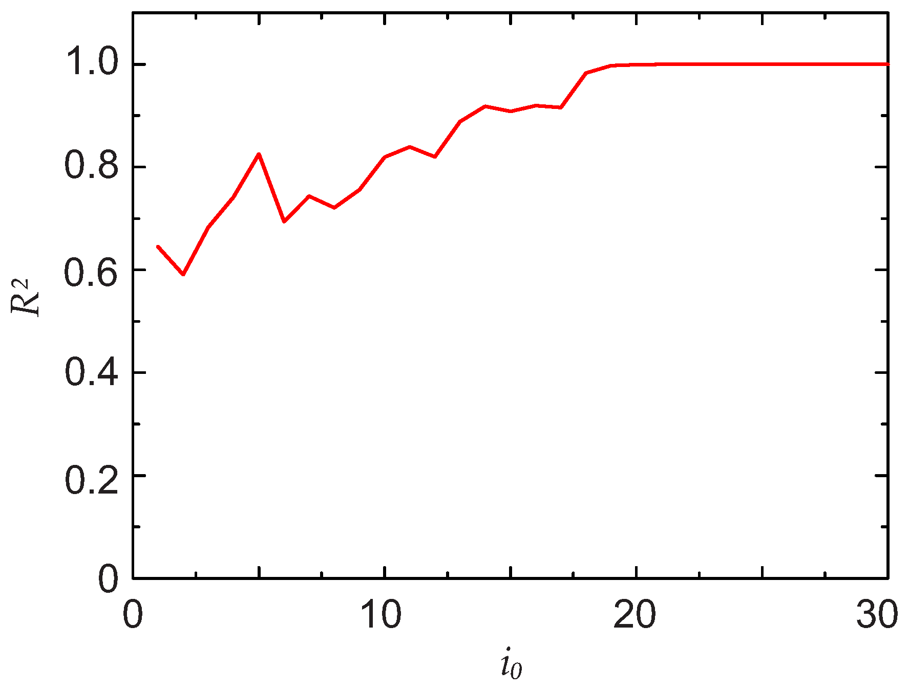
Rsquared can be chosen depending on the application. For the curves shown in this paper, the loop was stopped for
Rlimit . An example of the evolution of
with increasing
is shown in
Figure 3. The data refer to the third scenario described later in
Section 3. Above
,
still continues to slightly increase, but the statistical goodness of the fit does not improve further.
2.5. Fit of DFT
The final step of the algorithm is to perform a nonlinear fit of the DFT for . Since the functional form of the DFT is known, this is a standard procedure that can be performed, for example, with least-square-fit routines and will not be discussed here. After the fit is determined without the need of doing an inverse Fourier transform since the functional form of is known.
2.6. Algorithm Applied to a Lorentzian Line Shape
In this section, the implementation of the algorithm for a Lorentzian signal is described as an example. This functional form was chosen because it describes the absorption lines of many gas molecules, as, for example, oxygen under atmospheric conditions. In other conditions, like at higher temperatures or lower pressures, the Gaussian contribution due to Doppler broadening cannot be neglected and a Voigt profile is a better description.
The Lorentzian function can be written as
with
. In this form,
and
represent the area and the HWHM of the line. Writing
in this form is particularly advantageous since in direct absorption spectroscopy the gas concentration can be determined directly from the area under the line, and is thus directly proportional to
. In this formulation,
is then a simple exponential
Thus, once the parameters
and
are determined from the fit of the DFT,
is known.
3. Application to Simulated Data
The novel algorithm was first applied to artificially simulated data to demonstrate its functioning and its performance. Since the signal to be extracted
is known, it is possible to estimate the accuracy and robustness of the algorithm in the presence of backgrounds with different characteristics. In particular, three scenarios with different types of periodic disturbances were simulated. The signal to be extracted,
, is for all three cases the same Lorentzian function written in the form of Equation (
6) with
and
. All three scenarios were chosen to reflect real cases that are typical of TDLAS.
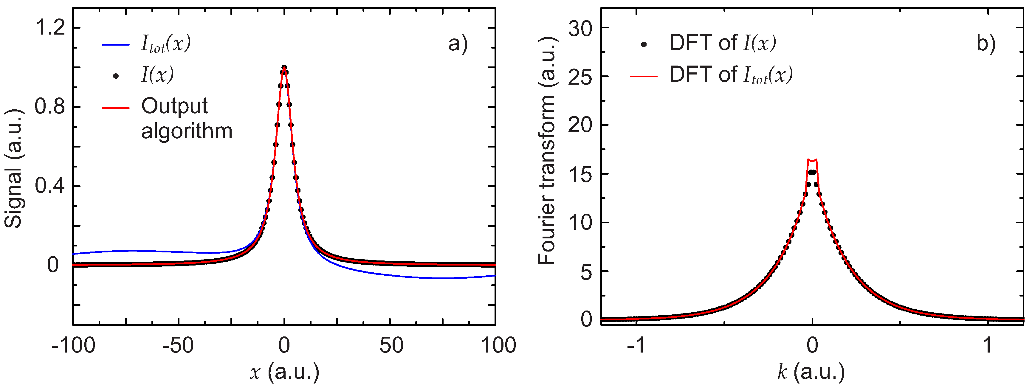
The first scenario is chosen to represent the experimental situation when the background has a periodic disturbance with an FSR comparable to the width of the line to be detected. This type of background is particularly problematic because it strongly affects the determination of the line shape. Furthermore, it cannot be removed by introducing a small jitter on the diode laser current and averaged out [
29] or be filtered out with standard post-processing methods, without introducing a significant distortion of the line shape. This type of background is taken here as a simple a cosine function
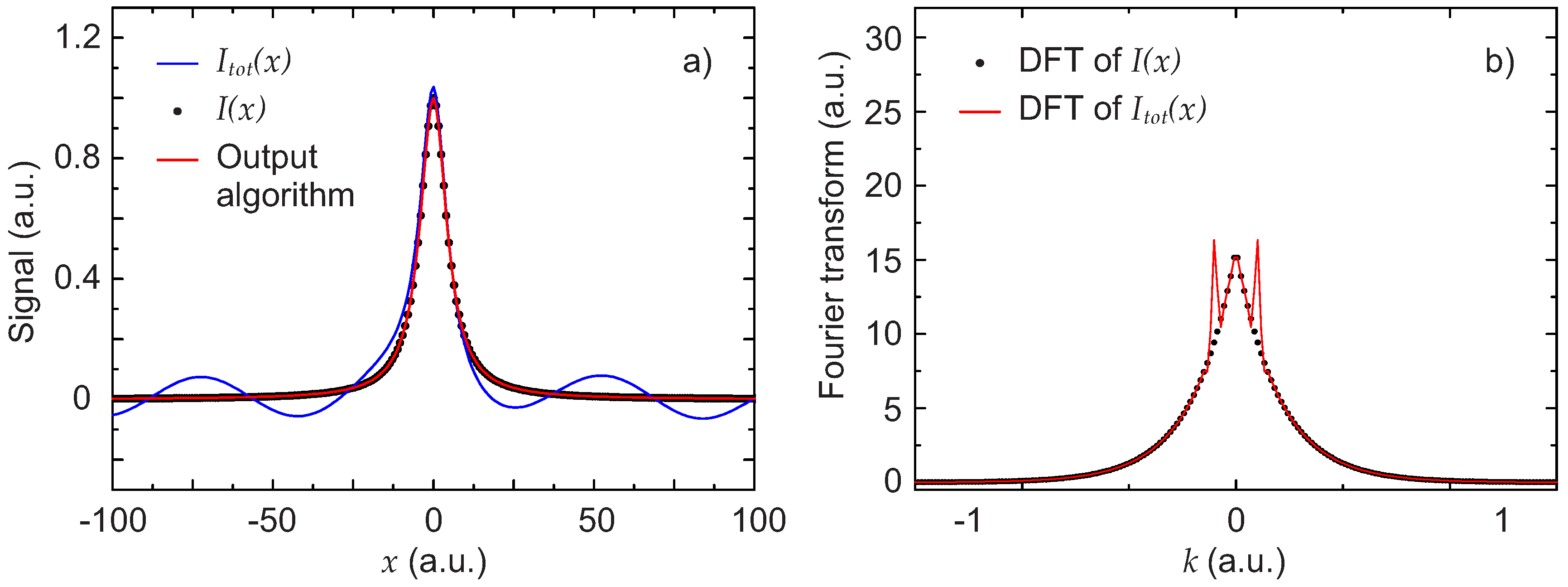
The total signal
in this case, together with the expected signal
are shown in
Figure 4a. Also shown is the result obtained by applying the described algorithm. Despite the problematic background, the output of the algorithm is practically identical to
. The percent deviation of the two parameters
and
describing the Lorentzian obtained with the algorithm from the initial value used to generate
is only of
for
and
for
.
To better illustrate the contribution of the background, the DFT of the Lorentzian and the DFT of the total signal signal are also shown in
Figure 4b. The two peaks visible in the figure represent the contribution of the background. With the pseudo-code algorithm described in
Section 2.1, the cut-off was
.
The second scenario discussed here is that of a background with a weak disturbance characterized by an FSR much larger than the line width and as large as or larger than the measuring range. This type of disturbance arises because of reflections between two surfaces separated by a very short physical dimension, like the laser-chip output face and the glass window of the laser packaging. The chosen functional form to simulate this scenario is the following:
The result of the algorithm for this scenario is shown in
Figure 5.
Figure 5a plots the total signal
, the expected signal
and the result obtained by applying the algorithm.
Figure 5b shows the DFT of the Lorentzian and the DFT of the total signal. The two peaks, due to the contribution of the background, are now very close to zero, which makes the extraction particularly unproblematic. With the pseudo-code algorithm described in
Section 2.1, the cut-off was
.
In this case, it is also clear from the figure that the algorithm extracts the signal exceedingly well. The percent deviation of the two parameters describing the Lorentzian obtained with the algorithm from the expected values is only of for and for .
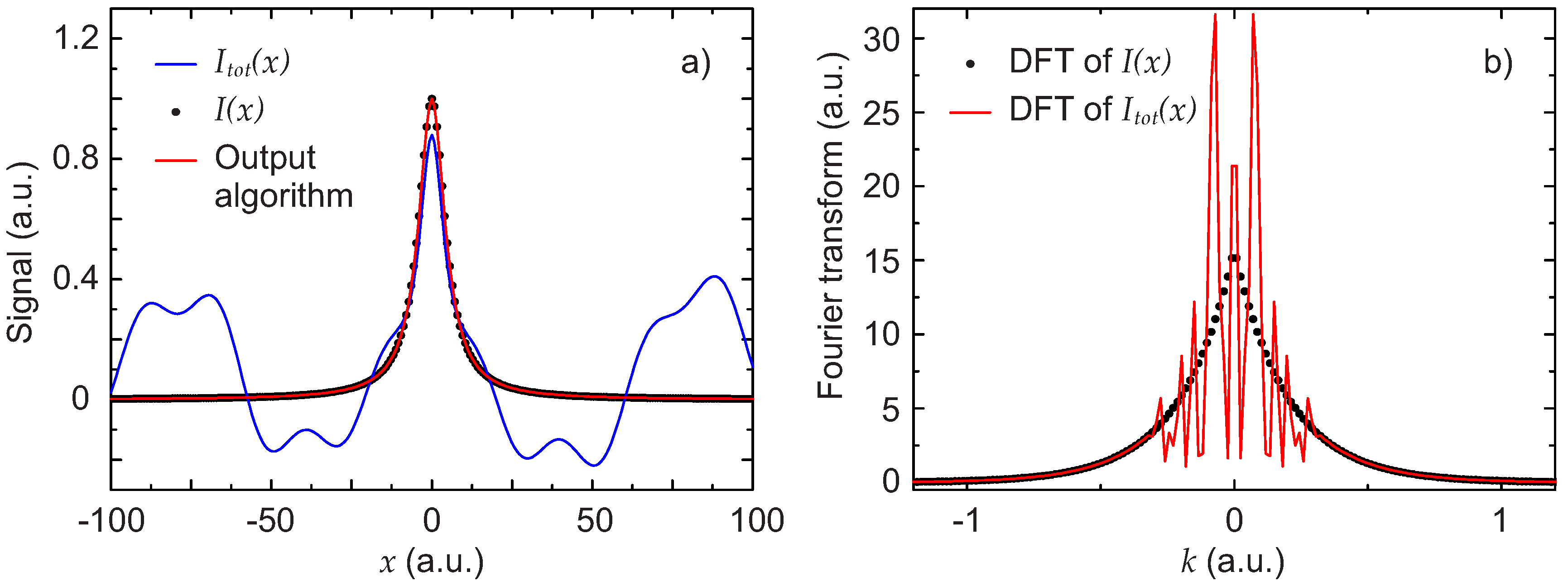
As a third scenario, a background resulting from the sum of a hundred cosine functions is considered. This less realistic case is chosen to demonstrate that, no matter how dramatic the interferences are, the algorithm can extract signal
very well. In addition, this scenario illustrates the case when the functional form of the background is too complex to be included in a nonlinear fit of
. The background is thus written as
where
is chosen randomly from a normal distribution with an average equal to zero and a standard deviation of
,
from a normal distribution with an average equal to zero and a standard deviation of
, and
from a normal distribution with an average equal to zero and a standard deviation of
.
Figure 6a shows the total signal
, the expected signal
and the result obtained by applying the described algorithm. Despite the very complicated background, the extraction of the signal
by the algorithm works very well. In
Figure 6b, the DFT of the Lorentzian and the DFT of the total signal are also shown. Due to the high number of cosine functions in the background, the DFT has a very structured shape. With the pseudo-code algorithm described in
Section 2.1, the cut-off was
(see also
Figure 3).
The percent deviation of the two parameters describing the Lorentzian obtained with the algorithm for this scenario is only of for and for . The deviation of both parameters is particularly low in this case. To better estimate the error and the standard deviation on the parameters, the method was applied to 500 functions created with the random sum of 100 cosines described above. Then, the error was evaluated and its distribution studied. As a result, has a mean value of the absolute value of the percentage error of 0.12% with a standard deviation of 0.19%, and a mean of 0.04% with a standard deviation of 0.06%.
Finally, the analysis of the algorithm with simulated data has allowed for determining the causes of the discrepancy between the parameters extracted with the algorithm and those of the starting function
. The main contribution to these arises from the approximation of the CFT by a DFT and is due to a rather large point spacing and limited x-range of
used in the simulated data. Smaller contributions arise from an imperfect window compensation, and a very small frequency folding [
30], which was neglected here. Since the purpose of this paper is to illustrate the algorithm and not to minimize the discrepancies, the simulated data were chosen to be as close as possible to typical experimental data. The application to the three scenarios demonstrate well how, even with a very complicated background like in the third one, the proposed algorithm can extract the underlying signal extremely well.
4. Experimental Results
To demonstrate the robustness of the method on real gas sensing measurements, absorption spectroscopy was performed on the three strong lines R9R9 (760.77 nm), R7Q8 (760.89 nm) and R7R7 (761.00 nm) of the O2 near infrared A-band in the presence of multiple interference fringes.
4.1. Experimental Setup
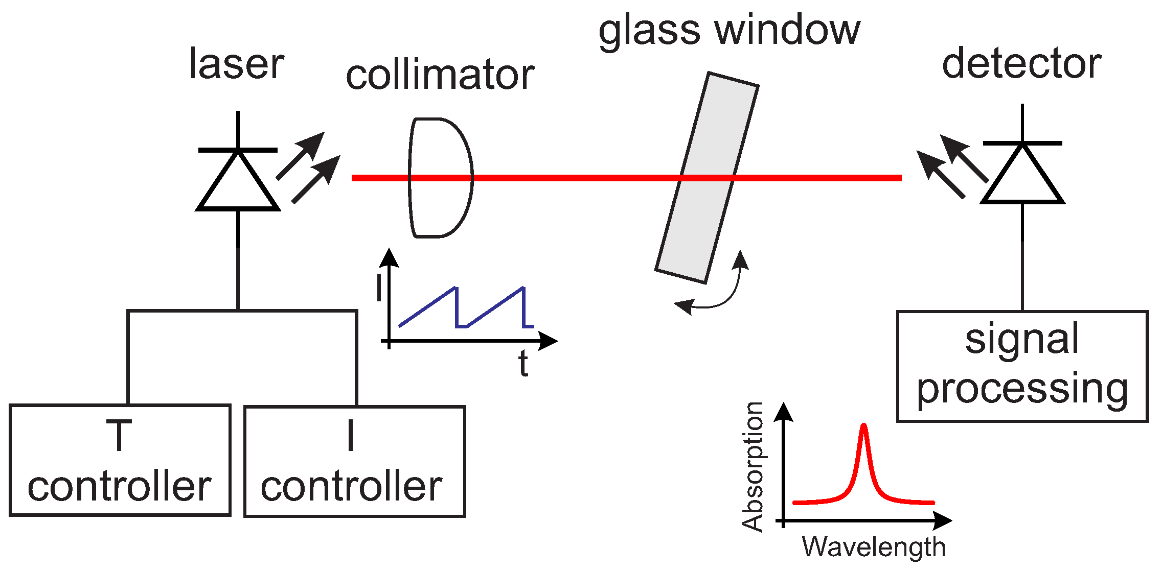
The setup for the absorption spectroscopy experiments was chosen to be extremely simple and is shown schematically in
Figure 7.
The light source is a 0.25 mW single-mode vertical-cavity surface-emitting laser (VCSEL) (760 nm TO5 VCSEL, Philips Photonics, Ulm, Germany) emitting at 760 nm. The laser current and temperature were adjusted by a temperature controller (TEC 2000, Thorlabs, Newton, NJ, USA) and a VCSEL laser diode controller (LDC 200C, Thorlabs, Newton, NJ, USA). The light emitted by the laser is collimated by a lens. The light transmitted by the sample is collected using a large-area Si 10 × 10 mm2 photodiode (FS1010, Thorlabs, Newton, NJ, USA), amplified by an adjustable-gain photodiode amplifier (PDA200C, Thorlabs, Newton, NJ, USA). The current ramp for the wavelength-sweep and the data acquisition were performed by a DAQ card (USB-6361, National Instruments Switzerland GmbH, Ennetbaden, Switzerland) using a LabviewTM software. The laser current sweep was chosen so to be able to measure three oxygen absorption lines. The total distance between the laser and the detector was kept fixed at approximately 36 cm. Interference fringes of adjustable intensity were generated by inserting and tilting a glass window of known material in the optical path. By varying the thickness of the glass window, it is possible to achieve fringes with different FSR; by tilting the glass window, it is possible to adjust the amplitude of the fringes. In this work, two glass windows of BK7 of thicknesses d = 11 mm (window 1) and d = 4 mm (window 2) were used. These two windows were chosen to create interferences fringes with FSR comparable to (window 1) and greater than (window 2) the line width of the signal. These types of interferences are the most disturbing because they cannot be easily eliminated—for example, by a small jitter in the laser current or by standard post-processing filtering.
4.2. Oxygen Sensing
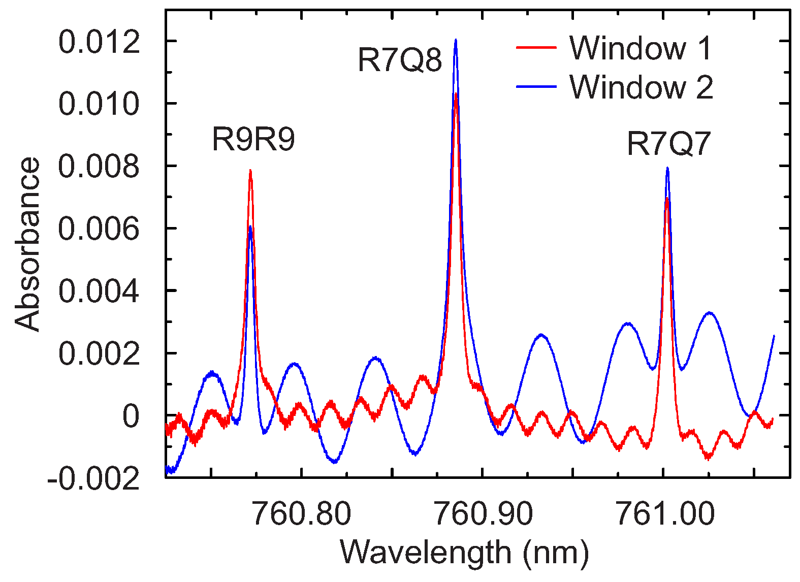
The absorbance signal of the three oxygen lines R9R9, R7Q8 and R7R7 is shown in
Figure 8. The interference fringes due to the glass window are clearly visible. Superimposed to these fringes, other minor ones are also visible, which are due to the glass window of the laser package and to the surfaces of the collimator. The zero-absorbance baseline arising from the nonlinear wavelength-dependent intensity of the laser was determined by a fourth-order polynomial fit over the entire sweep range. All the measurements reported in this work were performed in air, at room temperature and ambient pressure.
Both measurements shown in
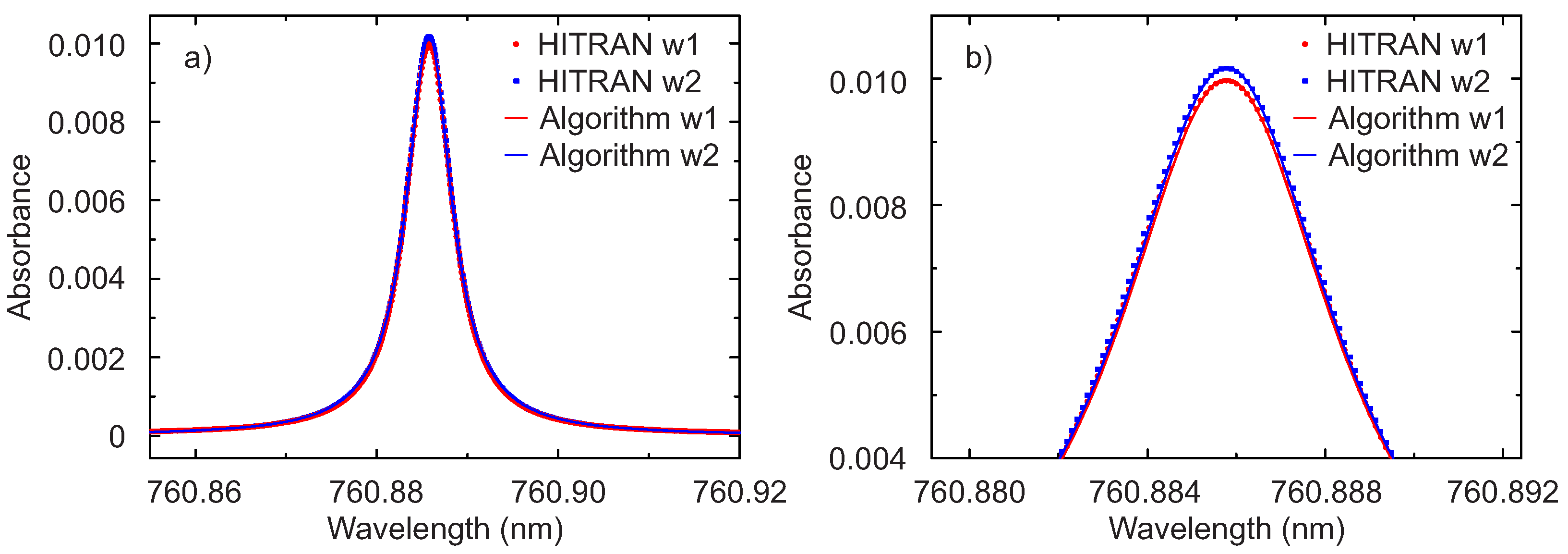
Figure 8 were processed with the proposed algorithm assuming a Lorentzian line shape. The results for the line R7Q8 is shown in
Figure 9. For comparison also the expected absorption lines based on the HITRAN 2012 database [
31] and determined using the application SpectraPlot [
32] are shown. It is evident from
Figure 9, and particularly from the enlargement in (b), that the algorithm extracts the absorption line extremely well. Differently from many fitting methods, the algorithm does not require neither input parameters nor initial values. The slightly lower peak height for the line in the presence of window 1 is due to the fact that the distance between laser and detector was kept fixed and window 1 is thicker, thus reducing the optical path length for oxygen absorption of
mm
mm. This difference in the HITRAN simulated curves was extracted correctly by the algorithm. To estimate the accuracy of the algorithm, the area under the absorption line from the HITRAN database calculated numerically was compared with the value of
extracted with the algorithm. For both measurements, the difference is 0.1%. There are still minimal deviations between the extracted and simulated lines, which could be reduced by considering a Voigt instead of a purely Lorentzian profile for the oxygen lines.
5. Conclusions
In this work, a novel semi-parametric algorithm is presented, which allows the extraction of a signal from an arbitrary background. In particular, the algorithm is applied to a background that is the sum of periodic interference fringes of different amplitudes and FSR. These types of disturbances, arising, for example, from multiple reflections between surfaces in the optical path, are of highest relevance for absorption spectroscopy because they are frequently the most common limit to gas sensor performance. The novel algorithm is firstly demonstrated on simulated data for three scenarios chosen to represent particularly relevant practical situations. In all three cases, the discrepancy between the results obtained with the algorithm and the expected values for the line parameters is very small—less than 0.3%. Then, the algorithm is applied to experimental data of oxygen absorption in the presence of multiple interferences. Despite the strong fringes, the extracted line shows a remarkable agreement with the expected curves from the HITRAN database, with deviation of the area of only 0.1%.
The great advantage of the algorithm is that it is semi-parametrical. This means that it requires no input parameters to extract the signal. This is clearly demonstrated by the third scenario with simulated data, where a background comprising a hundred cosine functions with different amplitudes, frequencies and phases could not be possibly modeled by standard nonlinear fits. In this work, the cut-off was determined dynamically by maximizing the coefficient of determination. Its recalculation at every measurement enables the accuracy achieved. This would be advantageous also in field applications, so that if the fringes should change in the time, the algorithm would automatically adjust the cut-off .
These results show that the performance of a very simple sensing setup, with standard anti-reflection coatings and minimal precautions to minimize the interference fringes, can be strongly improved by simply post processing the data with the proposed algorithm.
In this paper, the algorithm was applied to a Lorentzian line shape in direct absorption spectroscopy for oxygen concentration determination. However, it can be applied to account for other line shapes, for example a Voigt profile, or to signals with a different functional form, as arising, for example, from wavelength-modulation spectroscopy. Particularly in the case of fringes with large amplitudes and FSR of the order of the FWHM of the line, it can extract the desired signal very well, making the signal insensitive to fringes and their changes with time. Preliminary results on simulated data indicate that the algorithm performs equally well even if the signal amplitude is ten times smaller than the fringes. Further studies are needed to test the performance of the algorithm in similar extreme cases.
In conclusion, the presented algorithm, being able to extract the signal feature from an arbitrary background, has the potential to allow interference-immune TDLAS, solving long-time stability problems arising from changes over time of the background, like thermal drift. Furthermore, this algorithm is not specific of TDLAS and can be applied to any kind of spectroscopic data, provided the functional shape of the signal to be detected is known.


