
Effective Alternating Direction Optimization Methods for Sparsity-Constrained Blind Image Deblurring


Abstract
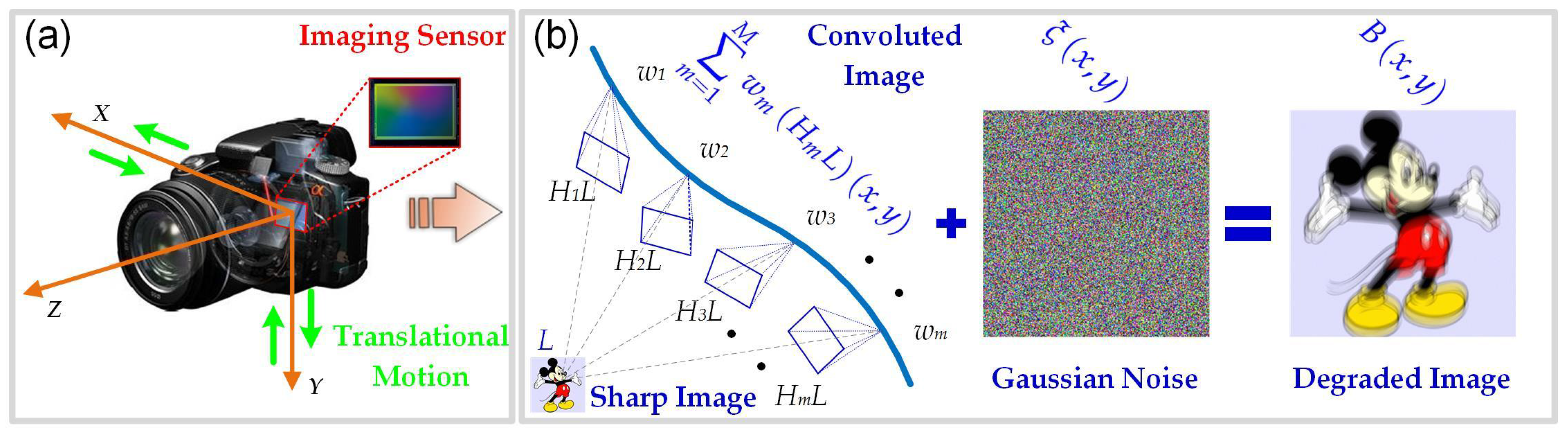
:1. Introduction
1.1. Background and Related Work
1.2. Motivation and Contributions
- To accurately estimate the blur kernel, a hybrid regularization method was proposed by combining the -norm of kernel intensity with the squared -norm of the intensity derivative. An alternating direction method was presented to effectively solve the resulting blur kernel estimation problem.
- The TGV-regularized variational model with an -norm data-fidelity term was proposed for enhancing the non-blind deconvolution result. To guarantee the stability and effectiveness of the solution, an ADMM-based numerical method was developed to solve the resulting non-smooth optimization problem.
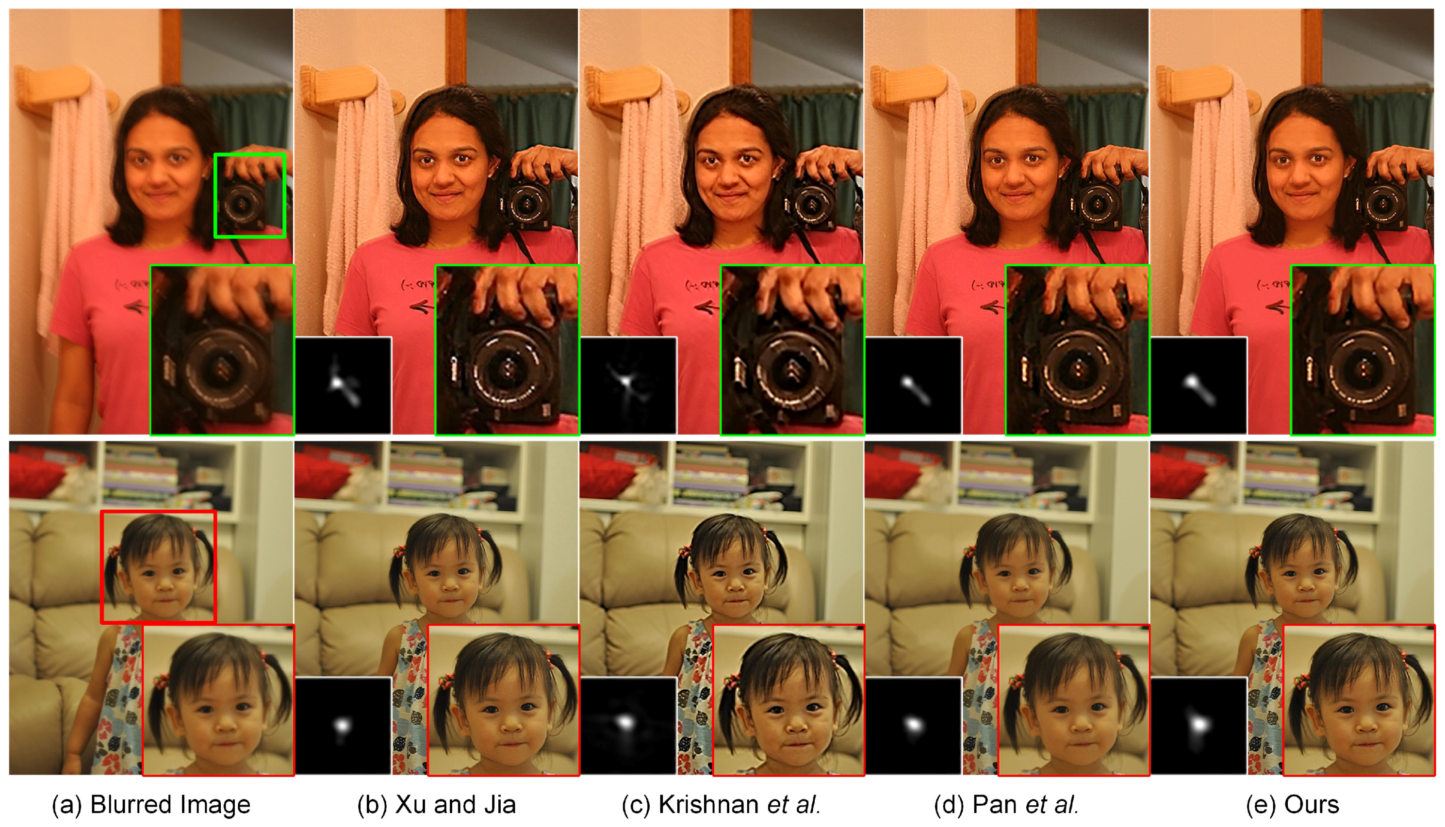
- The satisfactory blind deblurring performance of the proposed method has been illustrated using comprehensive experiments on both synthetic and realistic blurred images (with large blur kernels). The proposed method has also been successfully exploited for single-image deblurring in the field of ocean engineering.
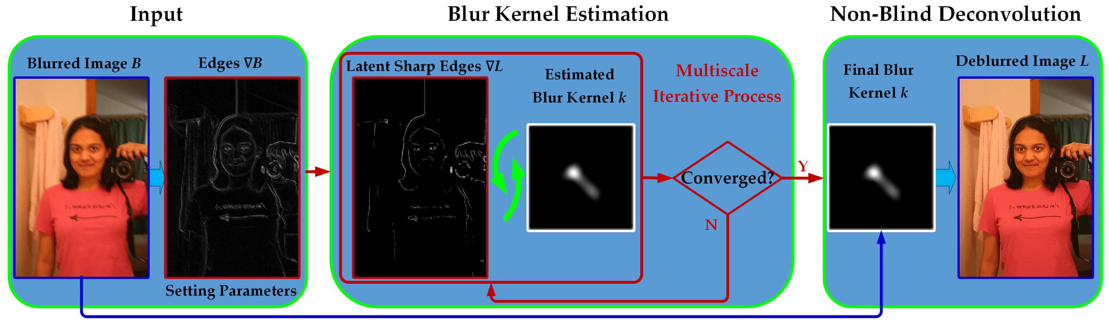
2. Hybrid Regularized Blur Kernel Estimation
2.1. Sharp Edge Restoration
| Algorithm 1 ADMM for Subproblem (6). |
2.2. Blur Kernel Estimation
| Algorithm 2 Hybrid regularized blur kernel estimation. |
|
3. Robust Non-Blind Deconvolution
3.1. -Subproblems
3.2. -Subproblems
3.3. Update the Lagrange Multipliers
| Algorithm 3 ADMM for the -TGV Model (20). |
|
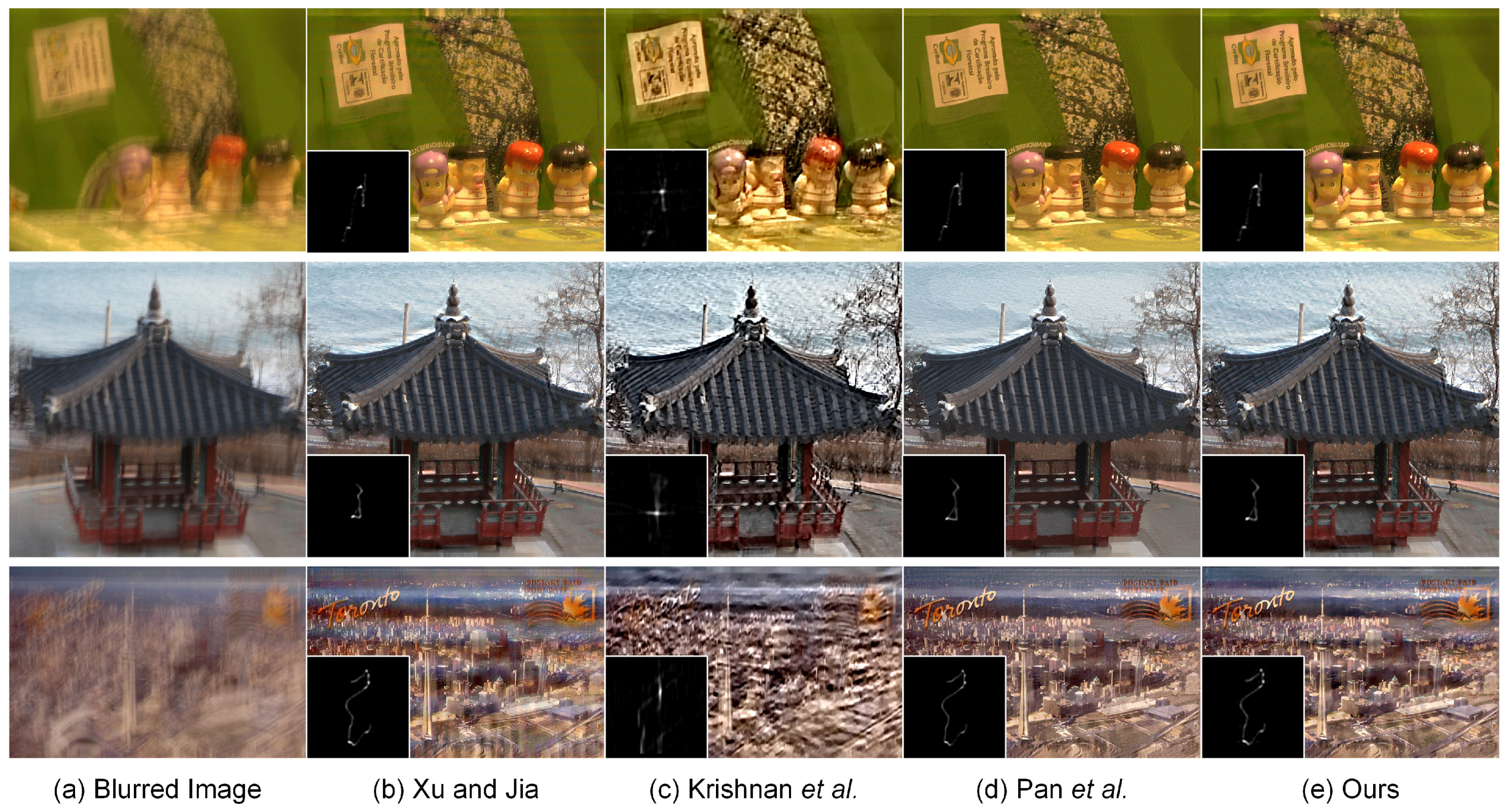
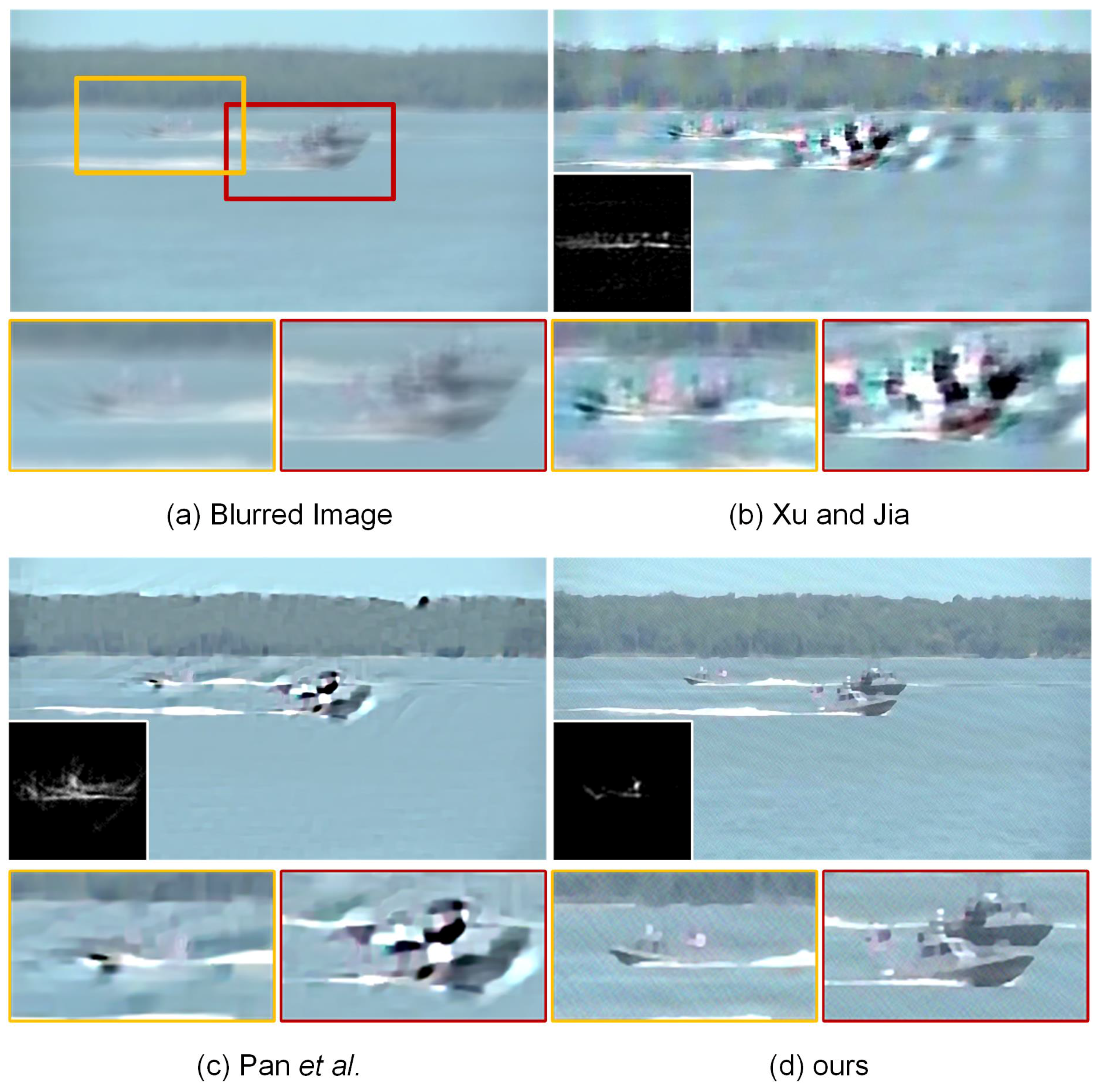
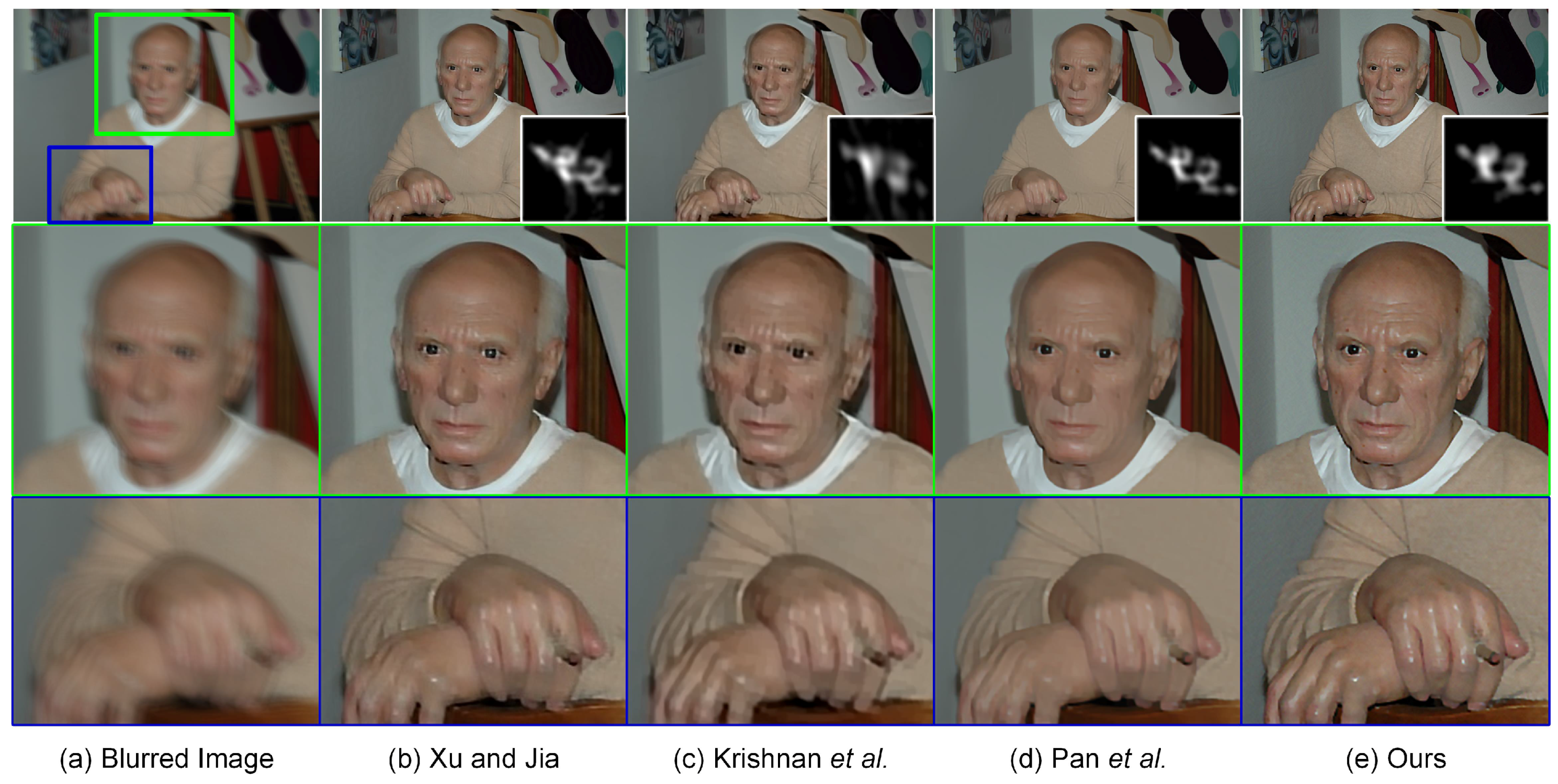
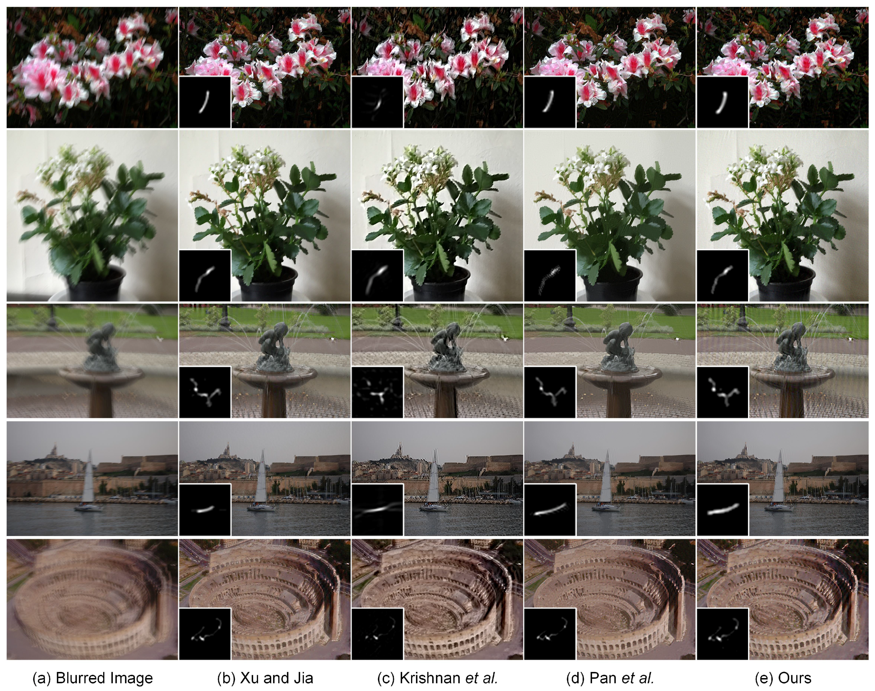
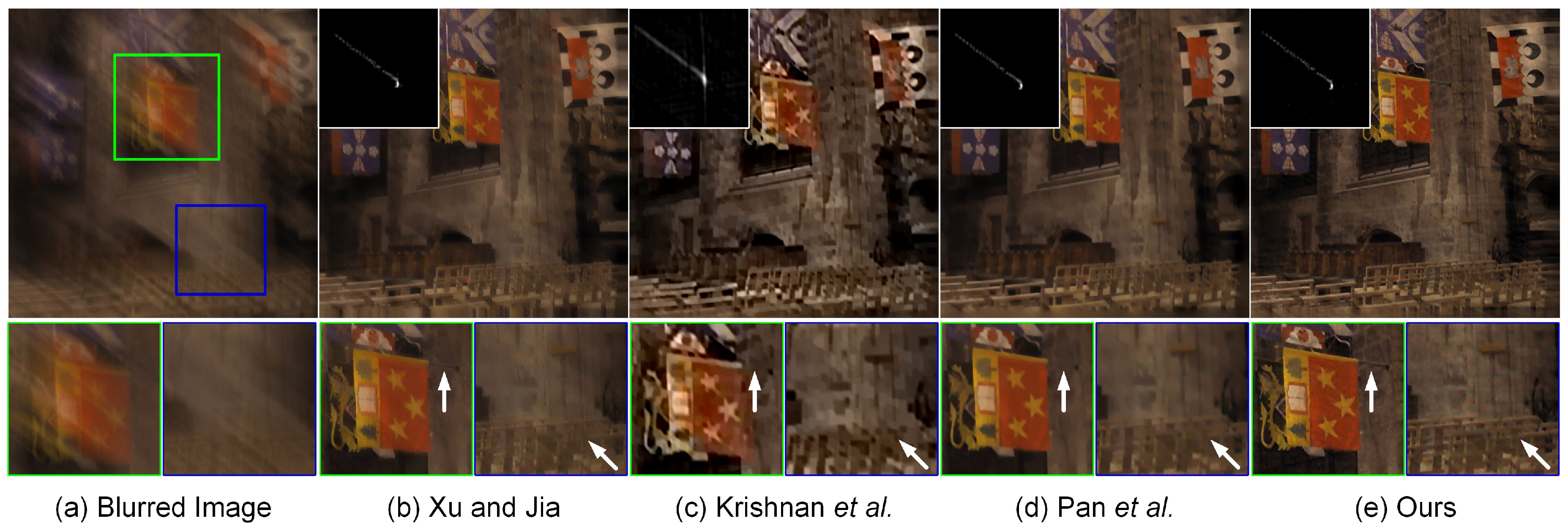
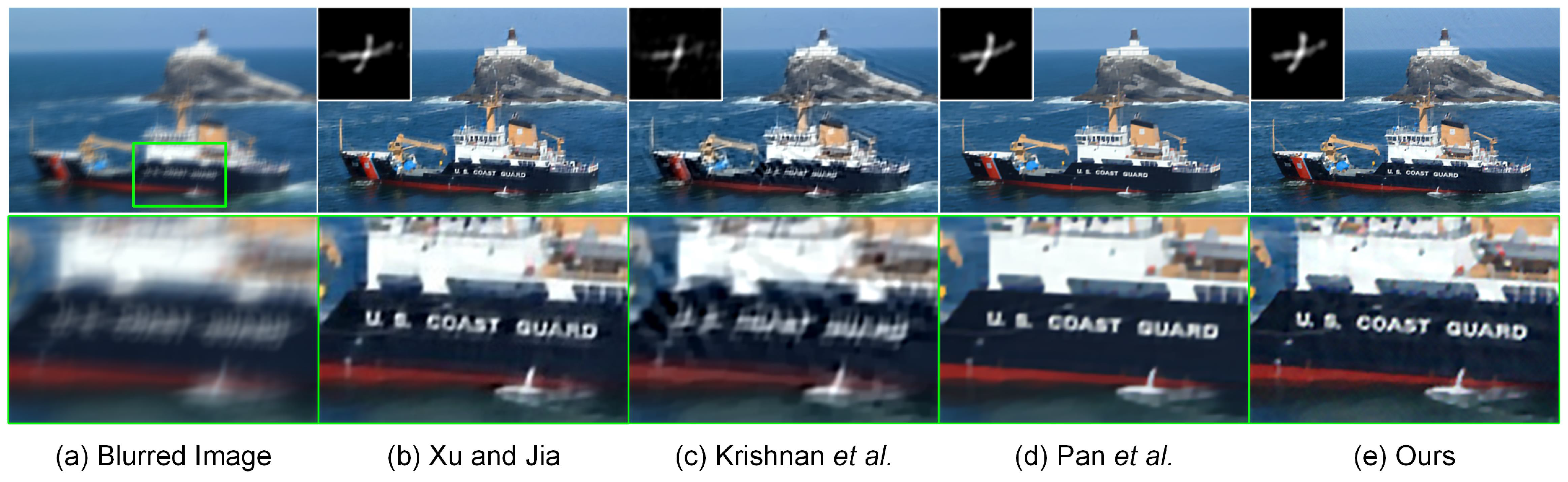
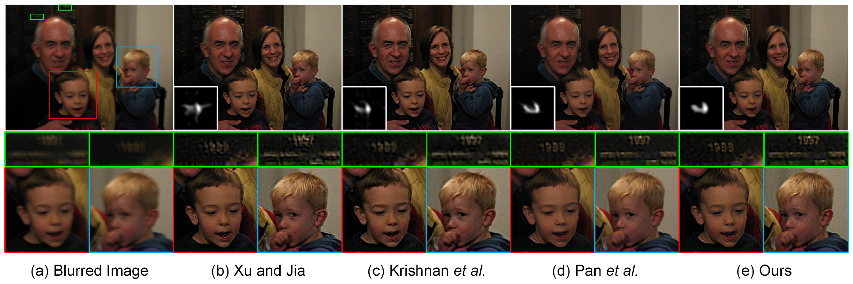
4. Experimental Results and Discussion
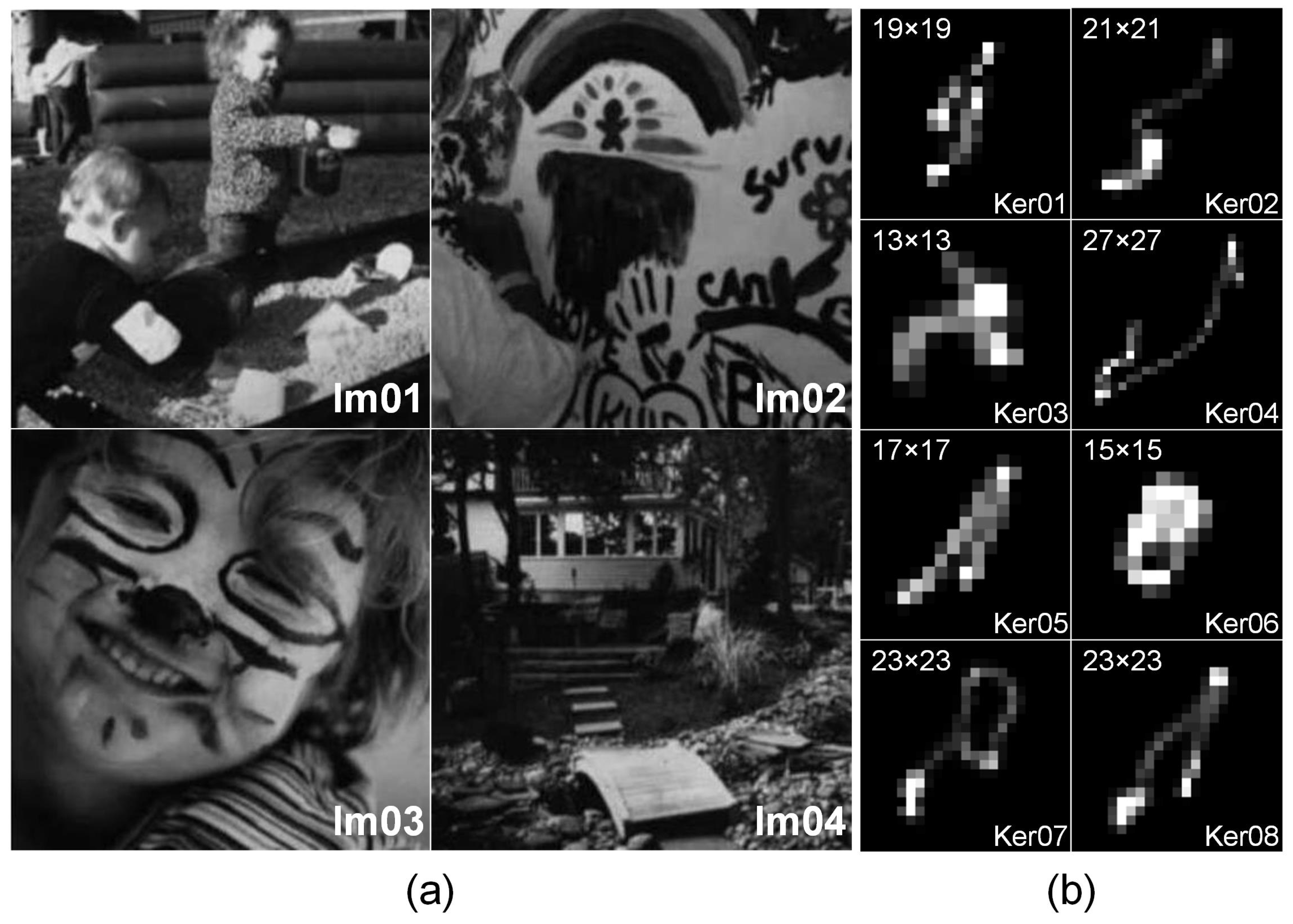
4.1. Experimental Settings
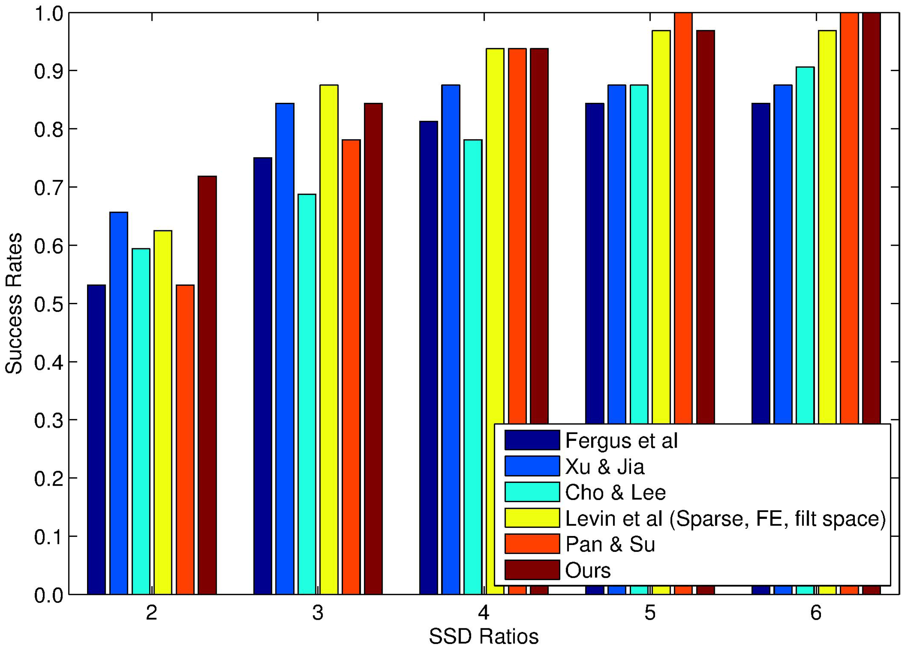
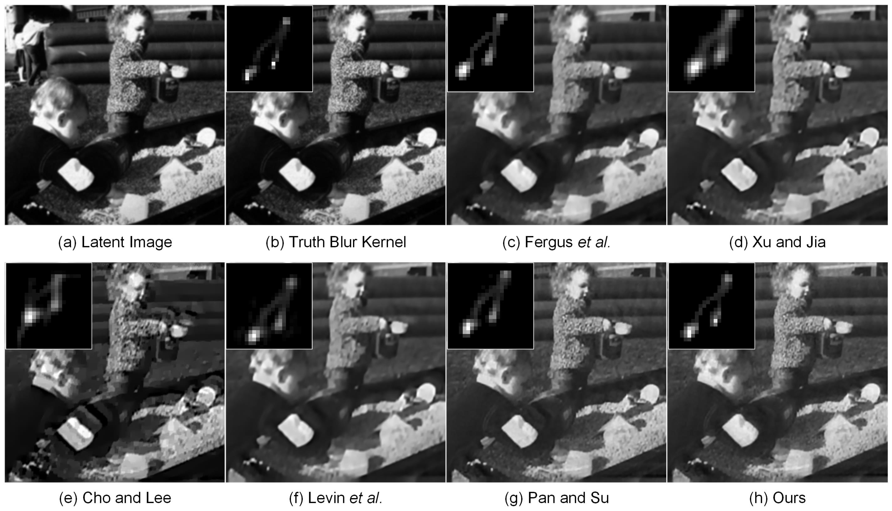
4.2. Experiments on Synthetically-Blurred Images
4.3. Experiments on a Large Blur Kernel
4.4. Experiments on Ocean Engineering
4.5. Experiments on More Realistic Blurred Images
5. Conclusions and Future Work
- The constant parameters (i.e., and ) for both the -norm of kernel intensity and the squared -norm of intensity derivative in (3) are manually selected in our current work. Essentially, it is necessary to automatically and adaptively select the parameters according to the statistical properties of the blur kernel. For instance, if the blur kernel can be better sparsely represented in the spatial domain, should be larger; whereas plays a more important role if the blur kernel has a significant piecewise smooth structure. In our future work, an automatic estimation method should be developed to adaptively select the weighting parameters and in (3) to enhance the accuracy of blur kernel estimation.
- The single-image blind deblurring method proposed in this work is performed based on a common assumption that the blur kernel is uniform (i.e., spatially invariant) across the image plane. Recent work in the literature [2,60,61,62,63,64,65] has illustrated that the uniform simple assumption does not always hold in practice. To further enhance image quality, the assumption of the non-uniform (i.e., spatially variant) blur kernel has gained increasing attention in modern imaging sciences. In our opinion, the proposed hybrid regularized blur kernel estimation method discussed in Section 2 can be naturally extended to the case of non-uniform deblurring in future work.
Acknowledgments
Author Contributions
Conflicts of Interest
References
- Yang, F.; Huang, Y.; Luo, Y.; Li, L.; Li, H. Robust image restoration for motion blur of image sensors. Sensors 2016, 16, 845. [Google Scholar] [CrossRef] [PubMed]
- Cheong, H.; Chae, E.; Lee, E.; Jo, G.; Paik, J. Fast image restoration for spatially varying defocus blur of imaging sensor. Sensors 2015, 15, 880–898. [Google Scholar] [CrossRef] [PubMed]
- Ruiz, P.; Zhou, X.; Mateos, J.; Molina, R.; Katsaggelos, A.K. Variational Bayesian blind image deconvolution: A review. Digit. Signal Prog. 2015, 47, 116–127. [Google Scholar] [CrossRef]
- Levin, A.; Weiss, Y.; Durand, F.; Freeman, W.T. Understanding blind deconvolution algorithms. IEEE Trans. Pattern Anal. Mach. Intell. 2011, 33, 2354–2367. [Google Scholar] [CrossRef] [PubMed]
- Wang, C.; Yue, Y.; Dong, F.; Tao, Y.; Ma, X.; Clapworthy, G.; Ye, X. Enhancing Bayesian estimators for removing camera shake. Comput. Graph. Forum 2013, 32, 113–125. [Google Scholar] [CrossRef]
- Kundur, D.; Hatzinakos, D. Blind image deconvolution. IEEE Signal Process. Mag. 1996, 13, 43–64. [Google Scholar] [CrossRef]
- Fergus, R.; Singh, B.; Hertzmann, A.; Roweis, S.T.; Freeman, W.T. Removing camera shake from a single photograph. ACM Trans. Graph. 2006, 25, 787–794. [Google Scholar] [CrossRef]
- Shan, Q.; Jia, J.Y.; Agarwala, A. High-quality motion deblurring from a single image. ACM Trans. Graph. 2008, 28, 73. [Google Scholar]
- Krishnan, D.; Tay, T.; Fergus, R. Blind deconvolution using a normalized sparsity measure. In Proceedings of the 24th IEEE Conference on Computer Vision and Pattern Recognition, Colorado Springs, CO, USA, 20–25 June 2011; pp. 233–240.
- Kotera, J.; Šroubek, F.; Milanfar, P. Blind deconvolution using alternating maximum a posteriori estimation with heavy-tailed priors. In Proceedings of the 15th International Conference on Computer Analysis of Images and Patterns, York, UK, 27–29 August 2013; pp. 59–66.
- Xu, L.; Jia, J.Y. Two-phase kernel estimation for robust motion deblurring. In Proceedings of the 11th European Conference on Computer Vision, Crete, Greece, 5–11 September 2010; pp. 157–170.
- Cho, S.; Lee, S. Fast motion deblurring. ACM Trans. Graph. 2009, 28, 145. [Google Scholar] [CrossRef]
- Pan, J.S.; Su, Z.X. Fast l0-regularized kernel estimation for robust motion deblurring. IEEE Signal Process. Lett. 2013, 20, 841–844. [Google Scholar]
- Cai, J.F.; Ji, H.; Liu, C.; Shen, Z. Framelet-based blind motion deblurring from a single image. IEEE Trans. Image Process. 2012, 21, 562–572. [Google Scholar] [PubMed]
- Shao, W.Z.; Li, H.B.; Elad, M. Bi-l0-l2-norm regularization for blind motion deblurring. J. Vis. Commun. Image Represent. 2015, 33, 42–59. [Google Scholar] [CrossRef]
- Engl, H.W.; Hanke, M.; Neubauer, A. Regularization of Inverse Problems; Kluwer Academic Publishers: Dordrecht, Netherlands, 1996. [Google Scholar]
- Donatelli, M. A multigrid for image deblurring with Tikhonov regularization. Numer. Linear Algebr. Appl. 2015, 12, 715–729. [Google Scholar] [CrossRef]
- Hamarik, U.; Palm, R.; Raus, T. Extrapolation of Tikhonov regularization method. Math. Model. Anal. 2010, 15, 55–68. [Google Scholar] [CrossRef]
- Liu, W.; Wu, C.S. A predictor-corrector iterated Tikhonov regularization for linear ill-posed inverse problems. Appl. Math. Comput. 2013, 221, 802–818. [Google Scholar] [CrossRef]
- Lucy, L.B. An iterative technique for the rectification of observed distributions. Astro. J. 1974, 79, 745–754. [Google Scholar] [CrossRef]
- Wiener, N. Extrapolation, Interpolation, and Smoothing of Stationary Time Series; MIT Press: Cambridge, MA, USA, 1949. [Google Scholar]
- Yuan, L.; Sun, J.; Quan, L.; Shum, H.Y. Progressive inter-scale and intra-scale non-blind image deconvolution. ACM Trans. Graph. 2008, 27, 74. [Google Scholar] [CrossRef]
- Rudin, L.I.; Osher, S.; Fatemi, E. Nonlinear total variation based noise removal algorithms. Phys. D 1992, 60, 259–268. [Google Scholar] [CrossRef]
- Chan, T.F.; Wong, C.K. Total variation blind deconvolution. IEEE Trans. Image Process. 1998, 7, 370–375. [Google Scholar] [CrossRef] [PubMed]
- Babacan, S.D.; Molina, R.; Katsaggelos, A.K. Variational Bayesian blind deconvolution using a total variation prior. IEEE Trans. Image Process. 2009, 18, 12–26. [Google Scholar] [CrossRef] [PubMed]
- Krishnan, D.; Fergus, R. Fast image deconvolution using hyper-Laplacian priors. In Proceedings of the 23rd Annual Conference on Neural Information Processing Systems, Vancouver, BC, Canada, 7–9 December 2009; pp. 1033–1041.
- Chan, T.; Marquina, A.; Mulet, P. High-order total variation-based image restoration. SIAM J. Sci. Comput. 2000, 22, 503–516. [Google Scholar] [CrossRef]
- Stefan, W.; Renaut, R.A.; Gelb, A. Improved total variation-type regularization using higher order edge detectors. SIAM J. Imaging Sci. 2010, 3, 232–251. [Google Scholar] [CrossRef]
- Lysaker, M.; Tai, X.C. Iterative image restoration combining total variation minimization and a second-order functional. Int. J. Comput. Vis. 2006, 66, 5–18. [Google Scholar] [CrossRef]
- Liu, R.W.; Wu, D.; Wu, C.S.; Xu, T.; Xiong, N. Constrained nonconvex hybrid variational model for edge-preserving image restoration. In Proceedings of the 2015 IEEE International Conference on Systems, Man, and Cybernetics, Hong Kong, China, 9–12 October 2015; pp. 1809–1814.
- Papafitsoros, K.; Schönlieb, C.B. A combined first and second order variational approach for image reconstruction. J. Math. Imaging Vis. 2014, 48, 308–338. [Google Scholar] [CrossRef]
- Bredies, K.; Kunisch, K.; Pock, T. Total generalized variation. SIAM J. Imaging Sci. 2010, 3, 492–526. [Google Scholar] [CrossRef]
- Bredies, K.; Dong, Y.; Hintermüller, M. Spatially dependent regularization parameter selection in total generalized variation models for image restoration. Int. J. Comput. Math. 2013, 90, 109–123. [Google Scholar] [CrossRef]
- Liu, R.W.; Shi, L.; Yu, S.C.H.; Wang, D. Box-constrained second-order total generalized variation minimization with a combined L1,2 data-fidelity term for image reconstruction. J. Electron. Imaging 2015, 24, 033026. [Google Scholar] [CrossRef]
- Duan, J.; Lu, W.; Tench, C.; Gottlob, I.; Proudlock, F.; Samani, N.N.; Bai, L. Denoising optical coherence tomography using second order total generalized variation decomposition. Biomed. Signal Process. Control 2016, 24, 120–127. [Google Scholar] [CrossRef]
- Zhang, X.; Burger, M.; Bresson, X.; Osher, S. Bregmanized nonlocal regularization for deconvolution and sparse reconstruction. SIAM J. Imaging Sci. 2010, 3, 253–276. [Google Scholar] [CrossRef]
- Tang, S.; Gong, W.; Li, W.; Wang, W. Non-blind image deblurring method by local and nonlocal total variation models. Signal Process. 2014, 94, 339–349. [Google Scholar] [CrossRef]
- Liu, R.W.; Shi, L.; Yu, S.C.H.; Wang, D. A two-step optimization approach for nonlocal total variation-based Rician noise reduction in magnetic resonance images. Med. Phys. 2015, 42, 5167–5187. [Google Scholar] [CrossRef] [PubMed]
- Zhang, C.; Wu, D.; Liu, R.W.; Xiong, N. Non-local regularized variational model for image deblurring under mixed Gaussian-impulse noise. J. Internet Technol. 2015, 16, 1301–1320. [Google Scholar]
- Xu, L.; Lu, C.; Xu, Y.; Jia, J. Image smoothing via l0 gradient minimization. ACM Trans. Graph. 2011, 30, 174. [Google Scholar] [CrossRef]
- Xu, L.; Zheng, S.; Jia, J. Unnatural l0 sparse representation for natural image deblurring. In Proceedings of the 26th IEEE Conference on Computer Vision and Pattern Recognition, Portland, OR, USA, 23–28 June 2013; pp. 1107–1114.
- Pan, J.; Hu, Z.; Su, Z.; Yang, M.H. L0-regularized intensity and gradient prior for deblurring text images and beyond. IEEE Trans. Pattern Anal. Mach. Intell. 2016. [Google Scholar] [CrossRef]
- Boyd, S.; Parikh, N.; Chu, E.; Peleato, B.; Eckstein, J. Distributed optimization and statistical learning via the alternating direction method of multipliers. Found. Trends Mach. Learn. 2010, 3, 1–122. [Google Scholar] [CrossRef]
- Liu, R.W.; Wu, D.; Wu, C.S.; Xiong, N. Hybrid regularized blur kernel estimation for single-image blind deconvolution. In Proceedings of the 2015 IEEE International Conference on Systems, Man, and Cybernetics, Hong Kong, China, 9–12 October 2015; pp. 1815–1820.
- Liu, R.W.; Shi, L.; Huang, W.; Xu, J.; Yu, S.C.H.; Wang, D. Generalized total variation-based MRI Rician denoising model with spatially adaptive regularization parameters. Magn. Reson. Imaging 2014, 32, 702–720. [Google Scholar] [CrossRef] [PubMed]
- Liu, Q.; Lai, Z.; Zhou, Z.; Kuang, F.; Jin, Z. A truncated nuclear norm regularization method based on weighted residual error for matrix completion. IEEE Trans. Image Process. 2016, 25, 316–330. [Google Scholar] [CrossRef] [PubMed]
- Lu, Y.; Lai, Z.; Xu, Y.; Li, X.; Zhang, D.; Yuan, C. Low-rank preserving projections. IEEE Trans. Cybern. 2015, 46, 1900–1913. [Google Scholar] [CrossRef] [PubMed]
- Dong, B.; Zhang, Y. An efficient algorithm for l0 minimization in wavelet frame based image restoration. J. Sci. Comput. 2013, 54, 350–368. [Google Scholar] [CrossRef]
- Chan, R.H.; Tao, M.; Yuan, X.M. Constrained total variation deblurring models and fast algorithms based on alternating direction method of multipliers. SIAM J. Imaging Sci. 2013, 6, 680–697. [Google Scholar] [CrossRef]
- Lai, Z.; Xu, Y.; Chen, Q.; Yang, J.; Zhang, D. Multilinear sparse principal component analysis. IEEE Trans. Neural Netw. Learn. Syst. 2014, 25, 1942–1950. [Google Scholar] [CrossRef] [PubMed]
- Duan, J.; Pan, Z.; Zhang, B.; Liu, W.; Tai, X.C. Fast algorithm for color texture image inpainting using the non-local CTV model. J. Glob. Optim. 2015, 62, 853–876. [Google Scholar] [CrossRef]
- Figueiredo, M.A.; Bioucas-Dias, J.M. Restoration of Poissonian images using alternating direction optimization. IEEE Trans. Image Process. 2010, 19, 3133–3145. [Google Scholar] [CrossRef] [PubMed]
- Han, D.; Yuan, X.M. A note on the alternating direction method of multipliers. J. Optim. Theory Appl. 2012, 155, 227–238. [Google Scholar] [CrossRef]
- Knoll, F.; Bredies, K.; Pock, T.; Stollberger, R. Second order total generalized variation (TGV) for MRI. Magn. Reson. Med. 2011, 65, 480–491. [Google Scholar] [CrossRef] [PubMed]
- Valkonen, T.; Bredies, K.; Knoll, F. Total generalized variation in diffusion tensor imaging. SIAM J. Imaging Sci. 2013, 6, 487–525. [Google Scholar] [CrossRef]
- Lu, W.; Duan, J.; Qiu, Z.; Pan, Z.; Liu, R.W.; Bai, L. Implementation of high-order variational models made easy for image processing. Math. Meth. Appl. Sci. 2016, 39, 4208–4233. [Google Scholar] [CrossRef]
- Duan, J.; Pan, Z.; Yin, X.; Wei, W.; Wang, G. Some fast projection methods based on Chan-Vese model for image segmentation. EURASIP J. Image Video Process. 2014, 2014, 1–16. [Google Scholar] [CrossRef]
- Levin, A.; Weiss, Y.; Durand, E.; Freeman, W.T. Efficient marginal likelihood optimization in blind deconvolution. In Proceedings of the 24th IEEE Conference on Computer Vision and Pattern Recognition, Colorado Springs, CO, USA, 20–25 June 2011; pp. 2657–2664.
- Pan, J.; Sun, D.; Pfister, H.; Yang, M.H. Blind image deblurring using dark channel prior. In Proceedings of the 29th IEEE Conference on Computer Vision and Pattern Recognition, Las Vegas, NV, USA, 26 June–1 July 2016; pp. 1–9.
- Whyte, O.; Sivic, J.; Zisserman, A.; Ponce, J. Non-uniform deblurring for shaken images. Int. J. Comput. Vis. 2012, 98, 168–186. [Google Scholar] [CrossRef]
- Cho, S.; Cho, H.; Tai, Y.W.; Lee, S. Registration based non-uniform motion deblurring. Comput. Graph. Forum 2012, 31, 2183–2192. [Google Scholar] [CrossRef]
- Paramanand, C.; Rajagopalan, A.N. Non-uniform motion deblurring for bilayer scenes. In Proceedings of the 26th IEEE Conference on Computer Vision and Pattern Recognition, Portland, OR, USA, 23–28 June 2013; pp. 1115–1122.
- Sun, J.; Cao, W.; Xu, Z.; Ponce, J. Learning a convolutional neural network for non-uniform motion blur removal. In Proceedings of the 28th IEEE Conference on Computer Vision and Pattern Recognition, Boston, MA, USA, 7–12 June 2015; pp. 769–777.
- Sroubek, F.; Kamenicky, J.; Lu, Y.M. Decomposition of space-variant blur in image deconvolution. IEEE Signal Process. Lett. 2016, 23, 346–350. [Google Scholar] [CrossRef]
- Zhang, X.; Wang, R.; Jiang, X.; Wang, W.; Gao, W. Spatially variant defocus blur map estimation and deblurring from a single image. J. Vis. Commun. Image Represent. 2016, 35, 257–264. [Google Scholar] [CrossRef]


| Methods | Ker01 | Ker02 | Ker03 | Ker04 | Ker05 | Ker06 | Ker07 | Ker08 |
|---|---|---|---|---|---|---|---|---|
| Im02 | ||||||||
| Fergus et al. [7] | ||||||||
| Xu and Jia [11] | ||||||||
| Cho and Lee [12] | ||||||||
| Pan and Su [13] | ||||||||
| Levin et al. [58] | ||||||||
| Ours | ||||||||
| Im04 | ||||||||
| Fergus et al. [7] | ||||||||
| Xu and Jia [11] | ||||||||
| Cho and Lee [12] | ||||||||
| Pan and Su [13] | ||||||||
| Levin et al. [58] | ||||||||
| Ours | ||||||||
© 2017 by the authors; licensee MDPI, Basel, Switzerland. This article is an open access article distributed under the terms and conditions of the Creative Commons Attribution (CC-BY) license (http://creativecommons.org/licenses/by/4.0/).
Share and Cite
Xiong, N.; Liu, R.W.; Liang, M.; Wu, D.; Liu, Z.; Wu, H. Effective Alternating Direction Optimization Methods for Sparsity-Constrained Blind Image Deblurring. Sensors 2017, 17, 174. https://doi.org/10.3390/s17010174
Xiong N, Liu RW, Liang M, Wu D, Liu Z, Wu H. Effective Alternating Direction Optimization Methods for Sparsity-Constrained Blind Image Deblurring. Sensors. 2017; 17(1):174. https://doi.org/10.3390/s17010174
Chicago/Turabian StyleXiong, Naixue, Ryan Wen Liu, Maohan Liang, Di Wu, Zhao Liu, and Huisi Wu. 2017. "Effective Alternating Direction Optimization Methods for Sparsity-Constrained Blind Image Deblurring" Sensors 17, no. 1: 174. https://doi.org/10.3390/s17010174
APA StyleXiong, N., Liu, R. W., Liang, M., Wu, D., Liu, Z., & Wu, H. (2017). Effective Alternating Direction Optimization Methods for Sparsity-Constrained Blind Image Deblurring. Sensors, 17(1), 174. https://doi.org/10.3390/s17010174