Development of a GNSS Buoy for Monitoring Water Surface Elevations in Estuaries and Coastal Areas


Abstract
:1. Introduction
- (1)
- Virtual Base Station Real-Time Kinematics (VBS-RTK) technology is used for the meteo-oceanographic observations.
- (2)
- The GNSS buoy can receive signals from GPS and global navigation satellite system (GLONASS) and manage L1 and L2 signals.
- (3)
- The GNSS buoy is capable of observing tides and waves simultaneously.
- (4)
- The tidal datum is not influenced by variations in the Earth’s crust.
2. Methodology
2.1. VBS-RTK Positioning Technology
- (1)
- GNSS base station network: Each base station receives GNSS observation data and transmits raw data to the control center continuously. Currently 78 base stations are located in Taiwan.
- (2)
- Control center: The VBS-RTK control center for positioning computation used in this work is operated by the National Land Surveying and Mapping Center (NLSC), Ministry of the Interior, Taiwan. After 1 September 2014, the NLSC upgraded the network by replacing a GPS system with a GNSS system. Progressive infrastructure via overlaid technology, the commercial software developed by Trimble Navigation, is run in the center. This software includes three modules: Trimble Instrument Configurator, Trimble Ephemeris Download, and Trimble Streaming Manager. Their main functions are as follows:
- Connecting the control center and each reference station to enable the automatic receipt, storage, and compression of observations from each reference station.
- The software not terminating the receipt or compression of satellite signals from reference stations during data download.
- Monitoring the status of the GNSS receiver of each reference station. The GNSS receiver parameters may be configured including the cutoff angle and sampling interval, etc.
- According to the carrier phase observations, the software calculates continuously the error caused by the multipath, the ionosphere, troposphere, and ephemeris; as well as the integer ambiguity of the carrier phase of L1 and L2.
- Generating VBS data in Radio Technical Commission for Maritime Services (RTCM) format and transmitting them to the rover station.
- (3)
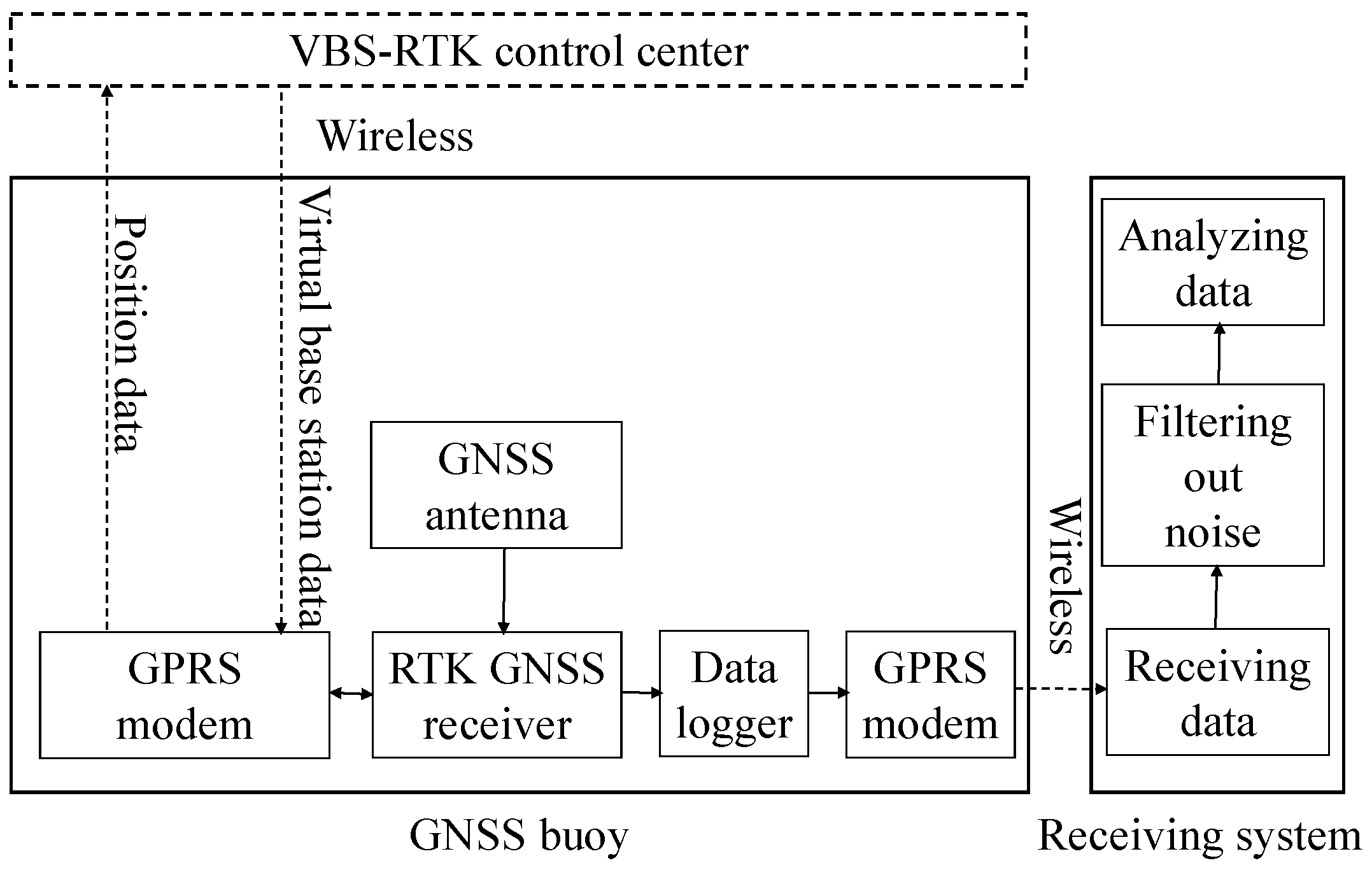
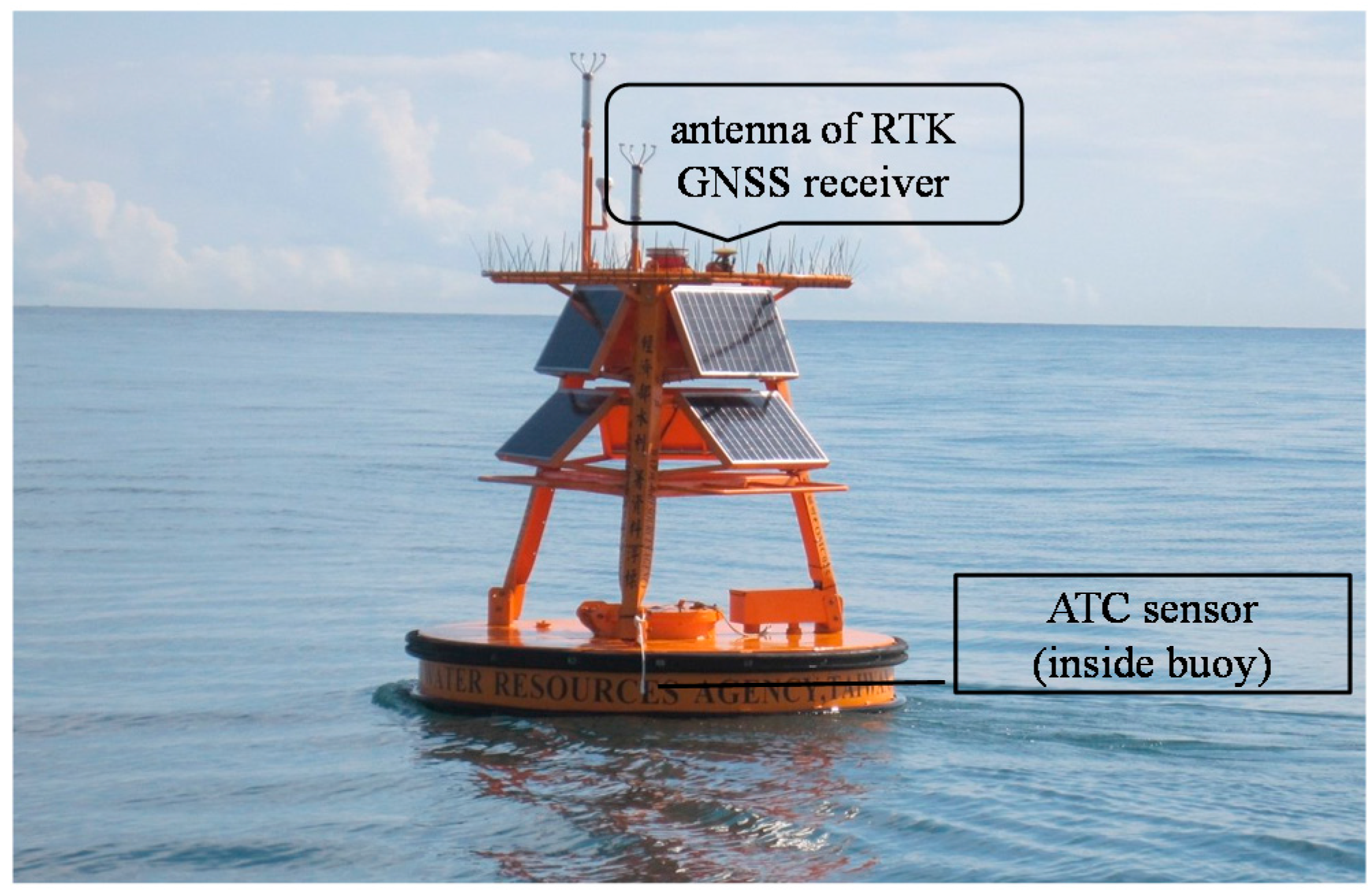
- Rover station: The rover station is a GNSS buoy with a GNSS receiver and a GNSS antenna attached to it.
- (1)
- Pre-process network observations: Establishing the network database and completing coordinate adjustments for each reference station.
- (2)
- Calculating data from regional stations: Collecting continuous observations and the accurate coordinate from each GNSS reference station, thereby establishing the Area Correction Parameters database.
- (3)
- Generating VBS data for the rover: The rover station reports approximate coordinates in National Marine Electronics Association format to the VBS-RTK control center. The VBS-RTK control center calculates the systematic error by interpolation and combines the error with the GNSS observations from the nearby reference station to produce VBS data. Then the VBS data are subsequently transmitted to the rover station in RTCM format.
- (4)
- Calculating the coordinate of the rover station: The rover station receives the VBS data and processes ultra-short-baseline RTK positioning.
2.2. Derivation of Water Surface Elevation
2.3. Determination of Directional Wave Spectra Using GNSS Data
2.4. Determination of Directional Wave Spectra Using ATC Data
3. Instrumentation, Results and Discussion
3.1. Instrumentation
3.2. Laboratory Tests
3.3. Field Tests
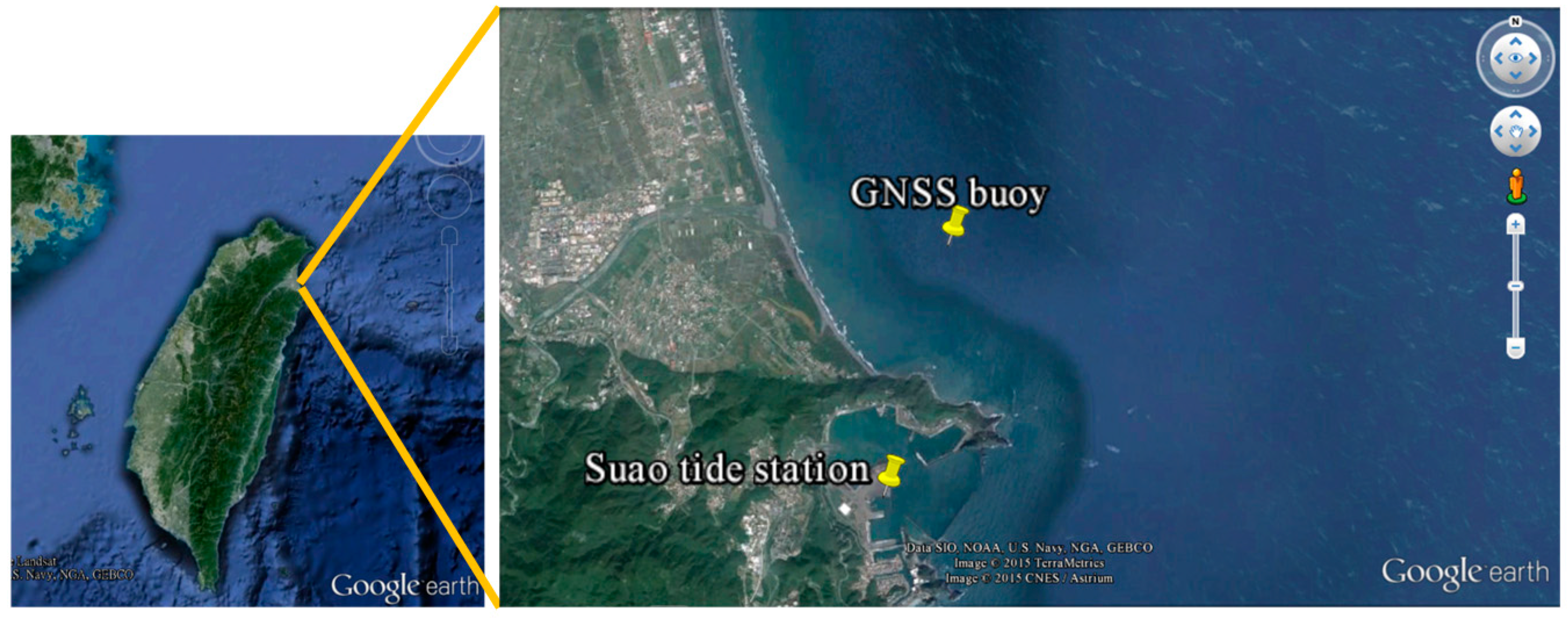
3.3.1. Deployment of the Buoy
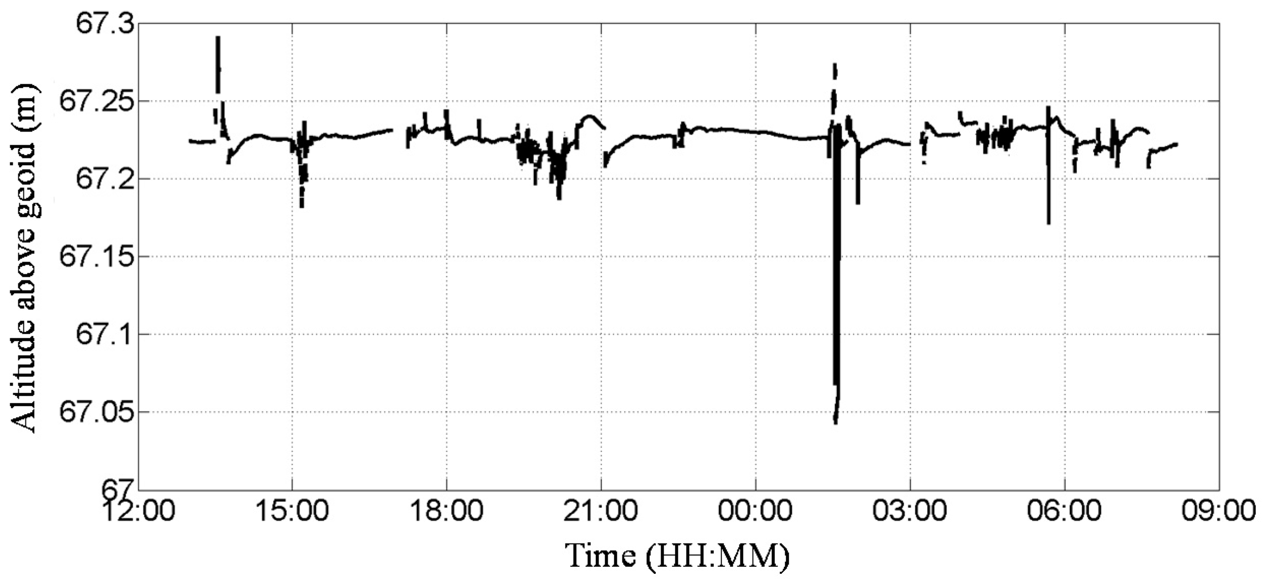
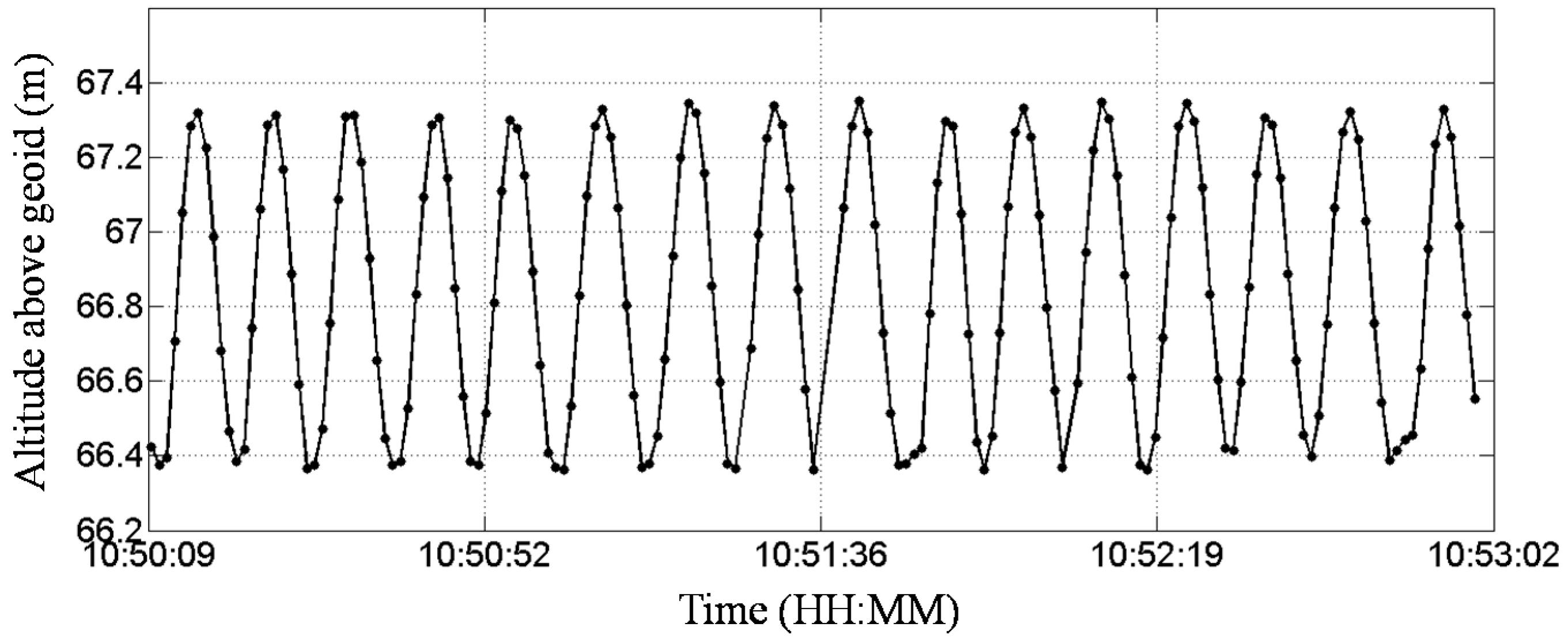
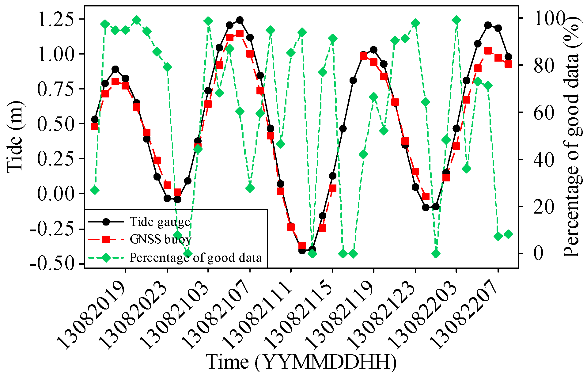
3.3.2. Tide Data
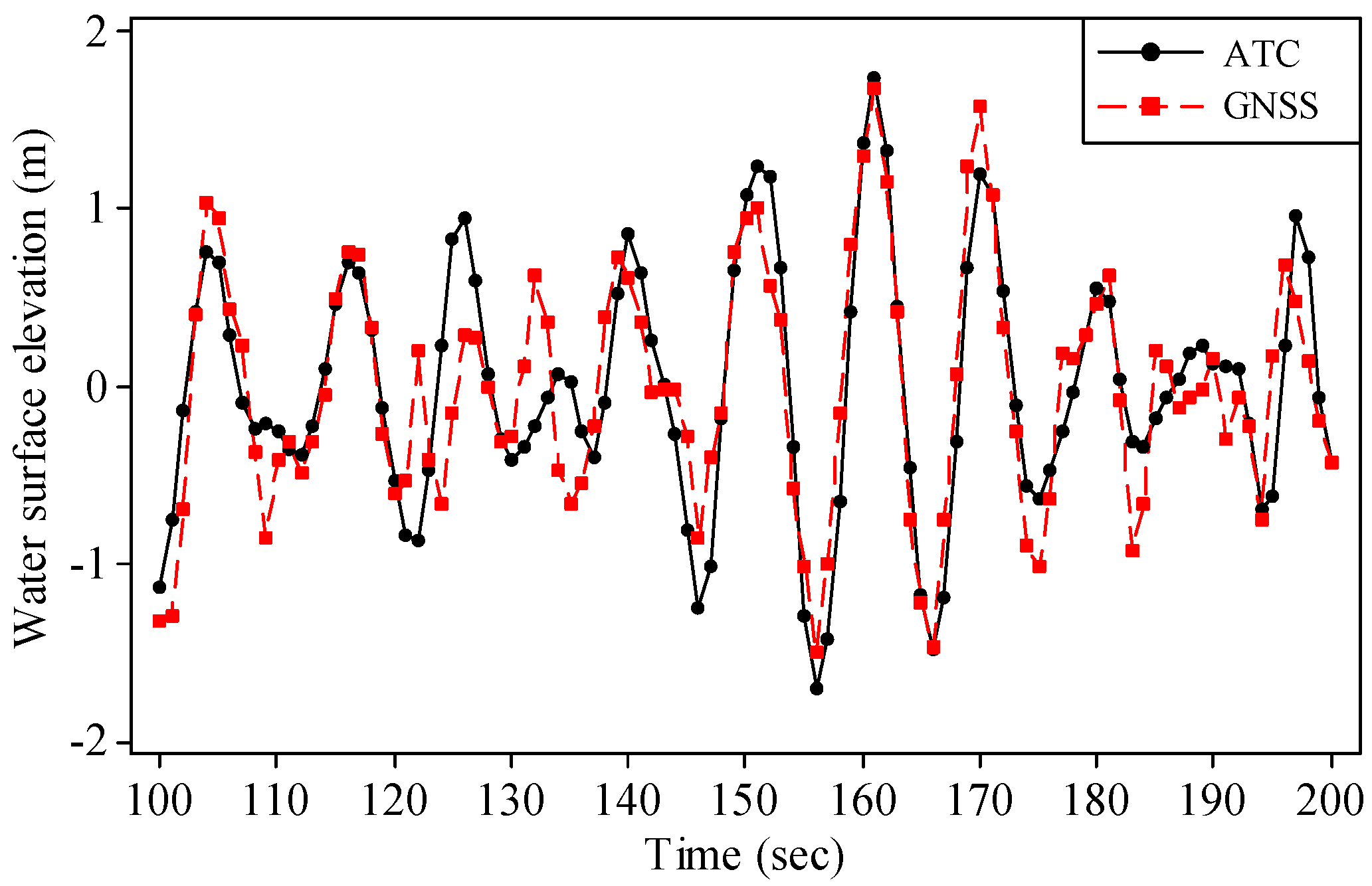
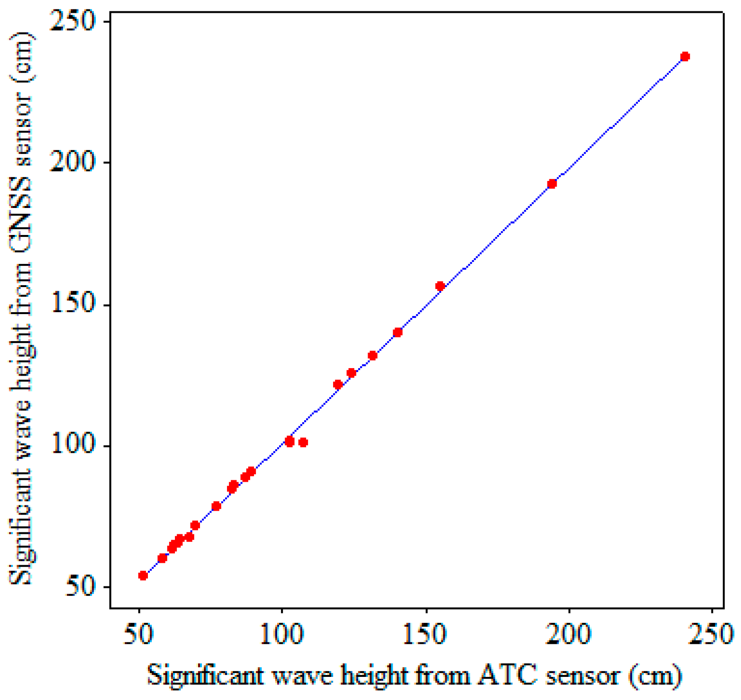
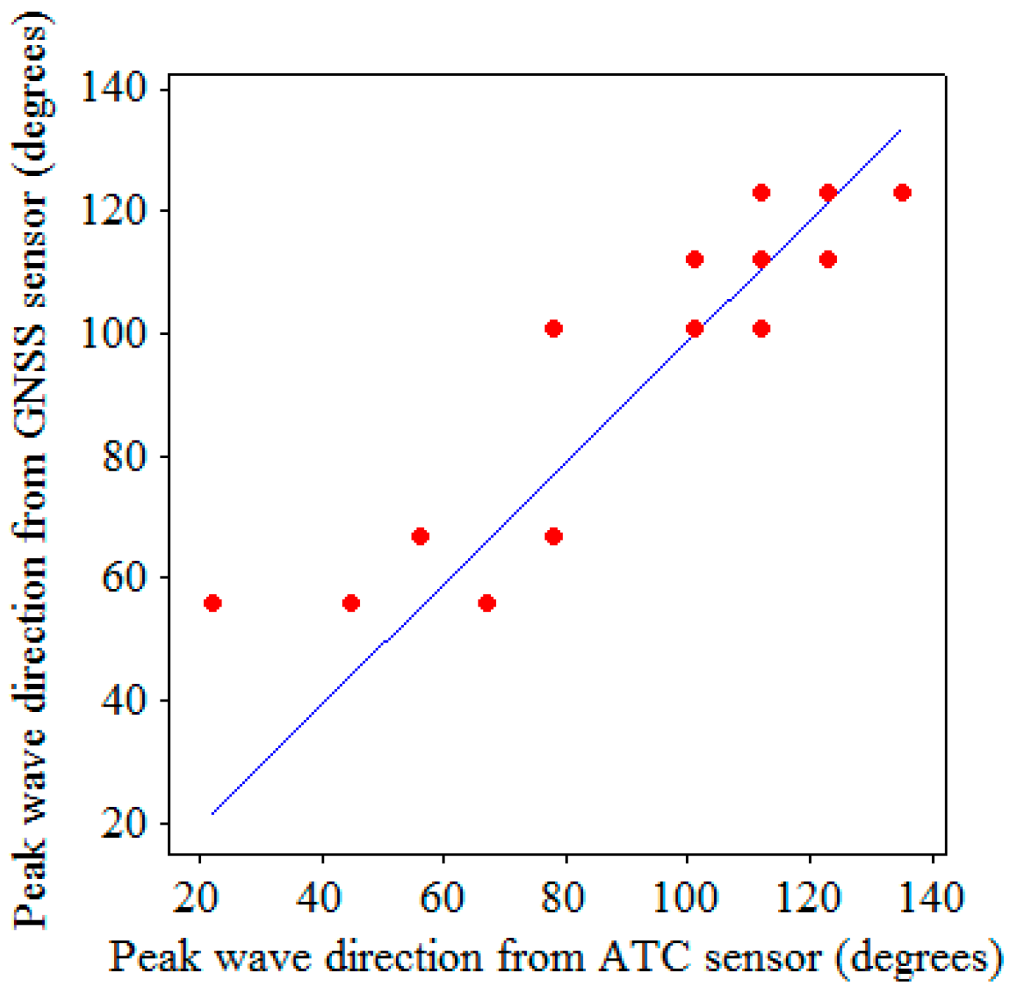
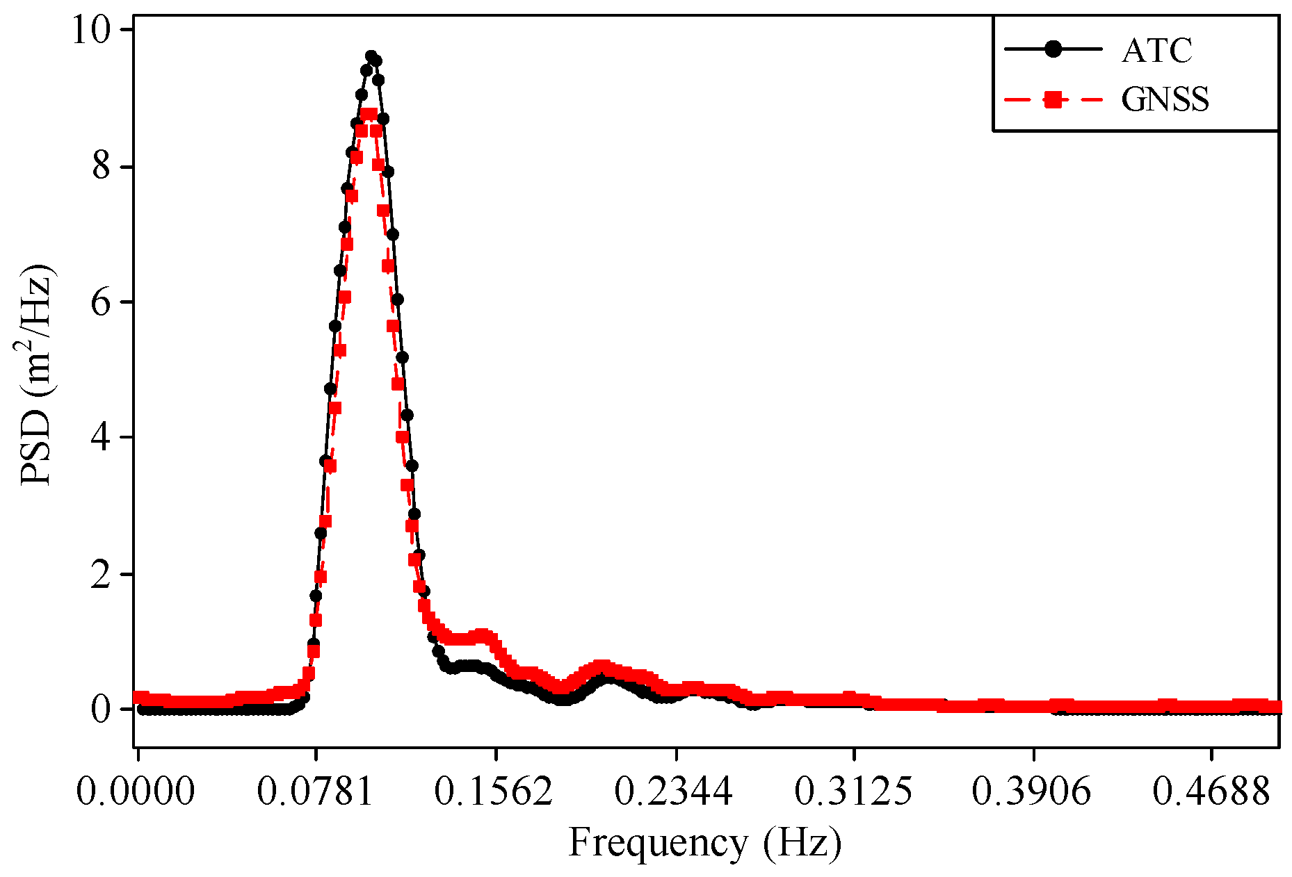
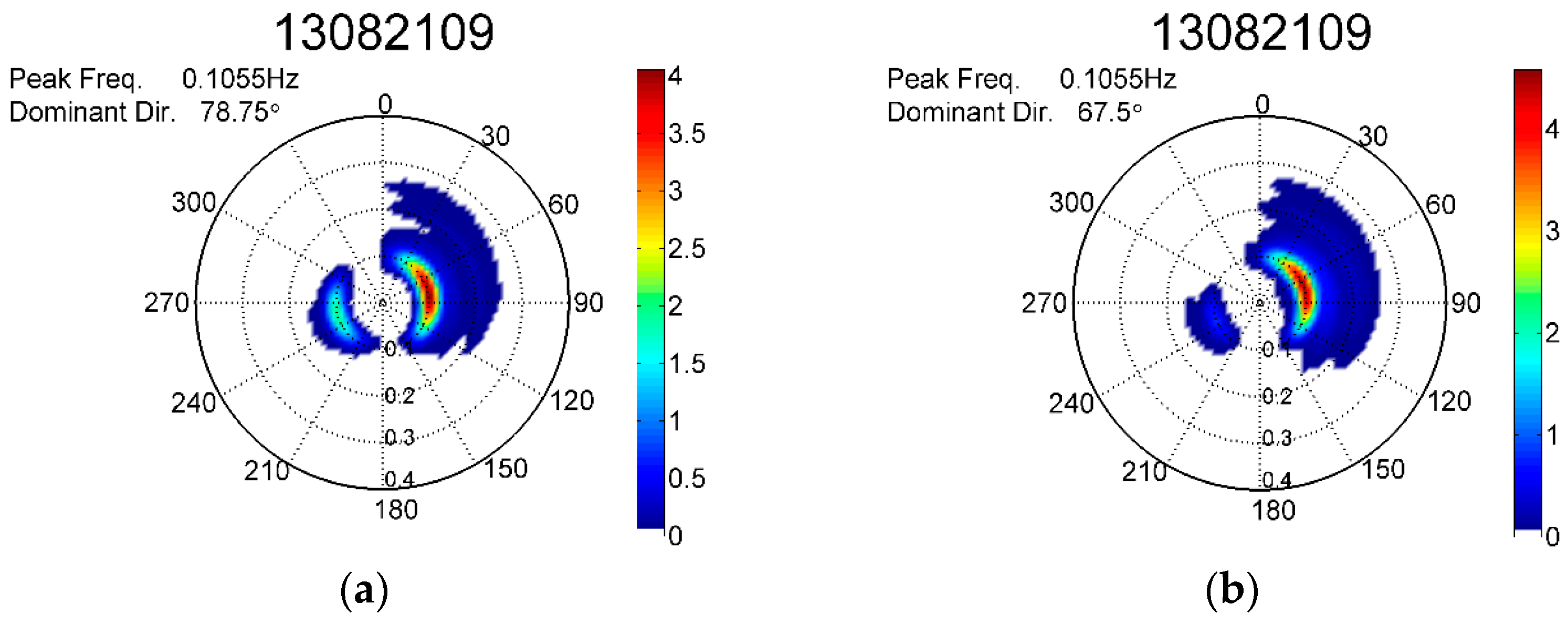
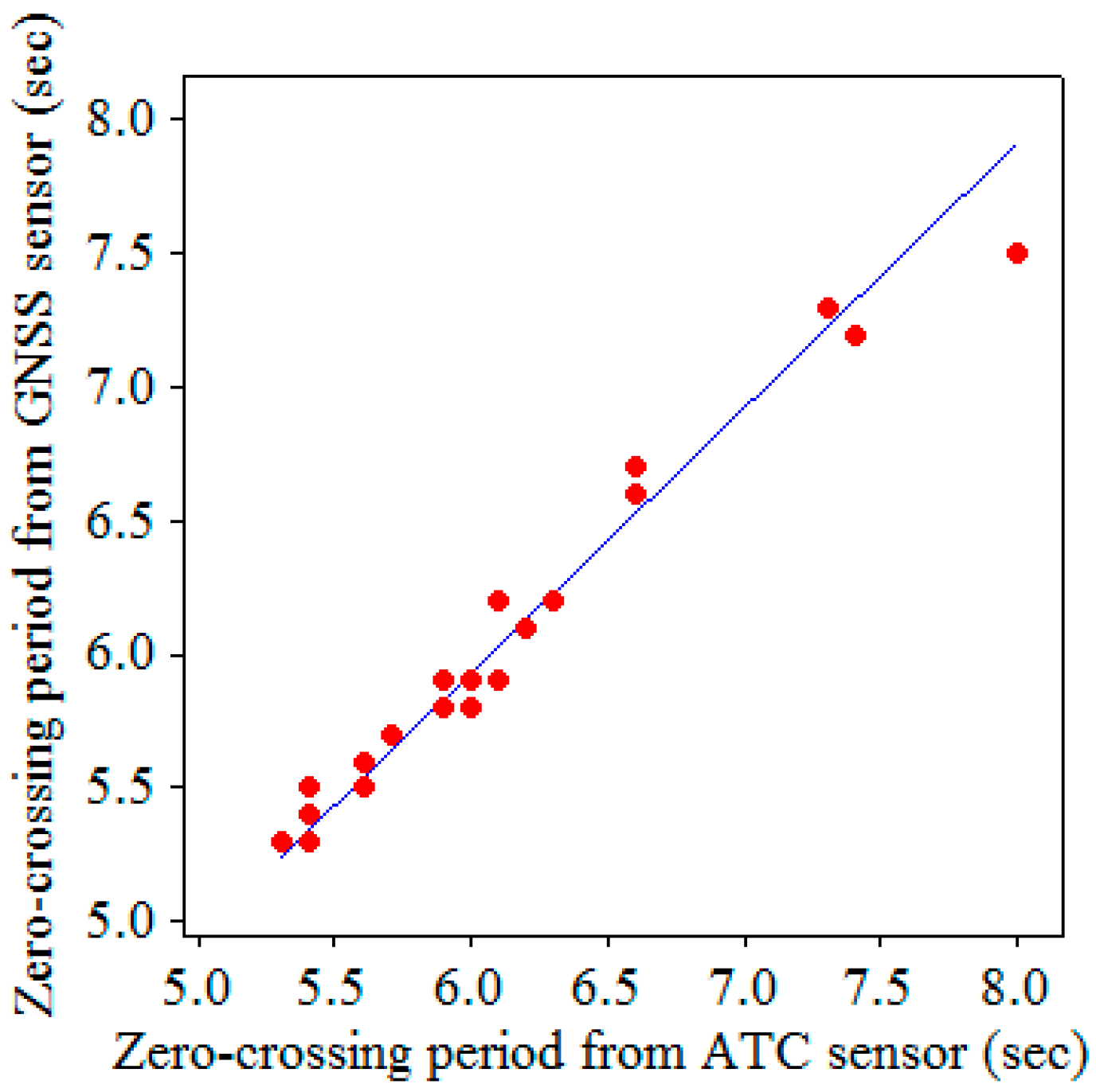
3.3.3. Wave Data
4. Conclusions
Acknowledgments
Author Contributions
Conflicts of Interest
Appendix A
- Determining the Fourier transform of the accelerationThe one-sided power spectrum, , the PSD, , and the phase spectrum, , of acceleration are determined as follows:and:where and are the real and imaginary parts of the Fourier transform of the acceleration time series data, respectively, and is the frequency resolution.
- Calculating the phase spectrum of the water surface elevationAccording to linear wave theory [27], the phase lag between the acceleration of a water particle and the water surface elevation is . The phase spectrum of the water surface elevation, , is then
- Filtering the noise in the acceleration signalsBecause the acceleration signals from the buoys are usually contaminated by noise, Lang [28] proposed an empirical noise correction function for the acceleration obtained by a data buoy. By applying the noise correction function, the noise can be filtered from the PSD of the acceleration. The noise correction function is a linearly decreasing function with respect to frequency and has the following form:where is a constant, is a function of and and must be determined, and are the PSDs of the acceleration at 0.01 and 0.02 Hz, respectively, is a fixed frequency, and is the frequency. Lang [28] provided various values of and for their discus buoys, which had diameters of 3 m, at different locations. F was set to 0.17 Hz for shallow water and 0.15 Hz for deep water. Because the buoy hull and the mooring line used for the present GNSS buoy are slightly different from those used by Lang [28], Kao et al. [22] modified the noise correction function of Lang [28] and suggested the following form for the buoy used in this work:where is the maximum PSD of the acceleration in the frequency range of 0–0.03 Hz, and is the frequency at which occurs.Accordingly, the modified PSD of the acceleration can be expressed as follows:and:where is the unmodified PSD of the acceleration. Note from Equation (A7b) that signals with frequencies less than 0.03 Hz, which corresponds to a period of 33.3 s, are ignored. Because the periods of typical water waves in the ocean are less than 20 s, ignoring those signals is reasonable.
- Determining the PSD of the water surface elevationsAccording to Hashimoto and Konbune [29], the PSD of the water surface elevations, , can be determined from that of the acceleration as follows:where is the angular frequency.
- Smoothing the PSD of the water surface elevationsData of 512 points with a time interval of 1 s are used in the fast Fourier transform (FFT). The frequency resolution is approximately 0.001953 Hz before smoothing. According to the spectral smoothing technique described in [30], the PSD of the water surface elevation is smoothed using a Bartlett window of 15 points. The degree of freedom of the PSD is 32. After smoothing, the frequency resolution of the PSD becomes 0.03125 Hz.
- Computing the wave height and periodThe significant wave height and zero-crossing period are calculated from the PSD of water surface elevations, , based on the method given by Earle [1].
- Calculating water surface elevationsThe inverse FFT is used to generate the time-series data of the water surface elevation from the smoothed PSD and phase spectrum of the water surface elevations.
Appendix B
References
- Earle, M.D. Nondirectional and Directional Wave Data Analysis Procedures; National Data Buoy Center, National Oceanic and Atmospheric Administration, U.S. Department of Commerce, Stennis Space Center: Hancock County, MS, USA, 1996.
- Kato, T.; Terada, Y.; Kinoshita, M.; Kakimoto, H.; Isshiki, H.; Moriguchi, T.; Takada, M.; Tanno, T.; Kanzaki, M.; Johnson, J. A new tsunami monitoring system using RTK-GPS. In Proceedings of the International Tsunami Symposium, Seattle, WA, USA, 7–10 August 2001; pp. 645–651.
- Nagai, T.; Kato, T.; Moritani, N.; Izumi, H.; Terada, Y.; Mitsui, M. Proposal of hybrid tsunami monitoring network system consisted of offshore, coastal and on-site wave sensors. Coast. Eng. J. 2007, 49, 63–76. [Google Scholar] [CrossRef]
- Harigae, M.; Yamaguchi, I.; Kasai, T.; Igawa, H.; Nakanishi, H.; Murayama, T.; Iwanaka, Y.; Suko, H. Abreast of the waves: Open-sea sensor to measure height and direction. GPS World 2005, 16, 16–26. [Google Scholar]
- Waseda, T.; Shinchi, M.; Nishida, T.; Tamura, H.; Miyazawa, Y.; Kawai, Y.; Ichikawa, H.; Tomita, H.; Nagano, A.; Taniguchi, K. GPS-based wave observation using a moored oceanographic buoy in the deep ocean. In Proceedings of the Twenty-First International Offshore and Polar Engineering Conference, Maui, HI, USA, 19–24 June 2011; International Society of Offshore and Polar Engineers: Mountain View, CA, USA, 2011; pp. 365–372. [Google Scholar]
- Falck, C.; Ramatschi, M.; Subarya, C.; Bartsch, M.; Merx, A.; Hoeberechts, J.; Schmidt, G. Near real-time GPS applications for tsunami early warning systems. Nat. Hazards Earth Syst. Sci. 2010, 10, 181–189. [Google Scholar] [CrossRef]
- Doong, D.J.; Lee, B.C.; Kao, C.C. Wave measurements using GPS velocity signals. Sensors 2011, 11, 1043–1058. [Google Scholar] [CrossRef] [PubMed]
- Herbers, T.; Jessen, P.; Janssen, T.; Colbert, D.; MacMahan, J. Observing ocean surface waves with GPS-tracked buoys. J. Atmos. Ocean. Technol. 2012, 29, 944–959. [Google Scholar] [CrossRef]
- Kuo, C.Y.; Chiu, K.W.; Chiang, K.W.; Cheng, K.C.; Lin, L.C.; Tseng, H.Z.; Chu, F.Y.; Lan, W.H.; Lin, H.T. High-frequency sea level variations observed by GPS buoys using precise point positioning technique. Terr. Atmos. Ocean. Sci. 2012, 23, 209–218. [Google Scholar] [CrossRef]
- Joodaki, G.; Nahavandchi, H.; Cheng, K. Ocean wave measurement using GPS buoys. J. Geod. Sci. 2013, 3, 163–172. [Google Scholar] [CrossRef]
- Dawidowicz, K. Sea level changes monitoring using GNSS technology—A review of recent efforts. Acta Adriat. 2014, 55, 145–161. [Google Scholar]
- Liu, Y.; Kerkering, H.; Weisberg, R.H. Coastal Ocean Observing Systems; Elsevier: London, UK, 2015. [Google Scholar]
- Wanninger, L. Introduction to Network RTK. IAG Working Group 4.5.1: Network RTK. 2008. Available online: http://www.wasoft.de/e/iagwg451/intro/introduction.html (accessed on 3 November 2016).
- Mervart, L.; Lukes, Z.; Rocken, C.; Iwabuchi, T. Precise Point Positioning with ambiguity resolution in real-time. In Proceedings of the ION GNSS 21st International Technical Meeting of the Satellite Division of the Institute of Navigation, Savannah, GA, USA, 16–19 September 2008; The Institute of Navigation, Inc.: Fairfax, VA, USA, September 2008; pp. 397–405. [Google Scholar]
- Wübbena, G.; Schmitz, M.; Bagge, A. PPP-RTK: Precise Point Positioning using state-space representation in RTK networks. In Proceedings of the 18th International Technical Meeting of the Satellite Division of the Institute of Navigation (ION GNSS 2005), Long Beach, CA, USA, 13–16 September 2005; pp. 2584–2594.
- Watson Industries, Inc. Strapdown Heading Reference Owner’s Manual, Rev D; Watson Industries, Inc.: Pomona, CA, USA, 2012. [Google Scholar]
- Landau, H.; Vollath, U.; Chen, X. Virtual reference stations versus broadcast solutions in network RTK-advantages and limitations. In Proceedings of the GNSS European Navigation, Graz, Austria, 22–24 April 2003.
- Kolb, P.F.; Chen, X.; Vollath, U. A new method to model the ionosphere across local area networks. Proc. ION GNSS 2005, 2005, 705–711. [Google Scholar]
- Trimble Navigation Limited. Support of Network Formats by Trimble GPSNET Network RTK Solution; Trimble Navigation Limited: Sunnyvale, CA, USA, 2005. [Google Scholar]
- Yeh, T.K.; Ding, X.L.; Hu, Y.S. Analysis of landslide monitoring using e-GPS system and multi-antenna GPS technology. IAHS Publ. 2010, 339, 374–379. [Google Scholar]
- Wu, C.T.; Hsiao, C.Y.; Hsieh, P.S. Using UAV and VBS-RTK for rapid reconstruction of environmental 3D elevation data of the Typhoon Morakot disaster area and disaster scale assessment. J. Chin. Soil Water Conserv. 2013, 44, 23–33. [Google Scholar]
- Kao, C.C.; Chien, H.; Chiou, M.D.; Chuang, L.Z.H. Error analysis of the wave directional spectrum measurement by disc buoys. Ocean Eng. 2003, 21, 24–33. (In Chinese) [Google Scholar]
- Topcon Positioning Systems Inc. GRIL Reference Manual; Topcon Positioning Systems, Inc.: Livermore, CA, USA, 2013. [Google Scholar]
- Topcon Positioning Systems, Inc. MR-1 Receiver Reference Guide, Rev A; Topcon Positioning Systems, Inc.: Livermore, CA, USA, 2012. [Google Scholar]
- Liu, Y.; MacCready, P.; Hickey, B.M.; Dever, E.P.; Kosro, P.M.; Banas, N.S. Evaluation of a coastal ocean circulation model for the Columbia River plume in summer 2004. J. Geophys. Res. Oceans 2009, 114. [Google Scholar] [CrossRef]
- Wang, C.; Weisberg, R.H.; Virmani, J.I. Western Pacific interannual variability associated with the El Niño-Southern Oscillation. J. Geophys. Res. Oceans 1999, 104, 5131–5149. [Google Scholar] [CrossRef]
- Dean, R.G.; Dalrymple, R.A. Water Wave Mechanics for Engineers and Scientists; Prentice-Hall: Englewood Cliffs, NJ, USA, 1984; pp. 79–80. [Google Scholar]
- Lang, N. The empirical determination of a noise function for NDBC buoys with strapped-down accelerometers. In Proceedings of the OCEANS’87, Halifax, NS, Canada, 28 September–1 October 1987; pp. 225–228.
- Hashimoto, N.; Konbune, K. Directional spectrum estimation from a Bayesian approach. Coast. Eng. Proc. 1988, 1, 62–76. [Google Scholar]
- University of Florida. OCP 6168: Data Analysis Techniques for Coastal and Ocean Engineers; University of Florida: Gainesville, FL, USA, 2011. [Google Scholar]
- Isobe, M.; Kondo, K.; Horikawa, K. Extension of MLM for estimating directional wave spectrum. In Proceedings of the Symposium on Description and Modeling of Directional Seas, Copenhagen, Denmark, 18–20 June 1984.


| Item | Parameter | Specification |
|---|---|---|
| Acceleration | range | ± 1 g |
| accuracy | ±10 mg | |
| bias | <±10 mg | |
| frequency response | 20 Hz | |
| Attitude | range | ±30° |
| accuracy | ±0.2° (to 20°), ±0.3° | |
| frequency response | 0.5 Hz | |
| Heading | range | 0~360° |
| accuracy | ±3.0° (magnetic inclination < 75°) | |
| frequency response | 10 Hz |
| Item | Specification |
|---|---|
| RTK | horizontal: 10 mm + 1.0 ppm (parts per million) × baseline length |
| vertical: 15 mm + 1.0 ppm × baseline length | |
| Velocity | 0.02 m/s (CEP) |
© 2017 by the authors; licensee MDPI, Basel, Switzerland. This article is an open access article distributed under the terms and conditions of the Creative Commons Attribution (CC-BY) license (http://creativecommons.org/licenses/by/4.0/).
Share and Cite
Lin, Y.-P.; Huang, C.-J.; Chen, S.-H.; Doong, D.-J.; Kao, C.C. Development of a GNSS Buoy for Monitoring Water Surface Elevations in Estuaries and Coastal Areas. Sensors 2017, 17, 172. https://doi.org/10.3390/s17010172
Lin Y-P, Huang C-J, Chen S-H, Doong D-J, Kao CC. Development of a GNSS Buoy for Monitoring Water Surface Elevations in Estuaries and Coastal Areas. Sensors. 2017; 17(1):172. https://doi.org/10.3390/s17010172
Chicago/Turabian StyleLin, Yen-Pin, Ching-Jer Huang, Sheng-Hsueh Chen, Dong-Jiing Doong, and Chia Chuen Kao. 2017. "Development of a GNSS Buoy for Monitoring Water Surface Elevations in Estuaries and Coastal Areas" Sensors 17, no. 1: 172. https://doi.org/10.3390/s17010172
APA StyleLin, Y.-P., Huang, C.-J., Chen, S.-H., Doong, D.-J., & Kao, C. C. (2017). Development of a GNSS Buoy for Monitoring Water Surface Elevations in Estuaries and Coastal Areas. Sensors, 17(1), 172. https://doi.org/10.3390/s17010172