
Near-Space TOPSAR Large-Scene Full-Aperture Imaging Scheme Based on Two-Step Processing


Abstract
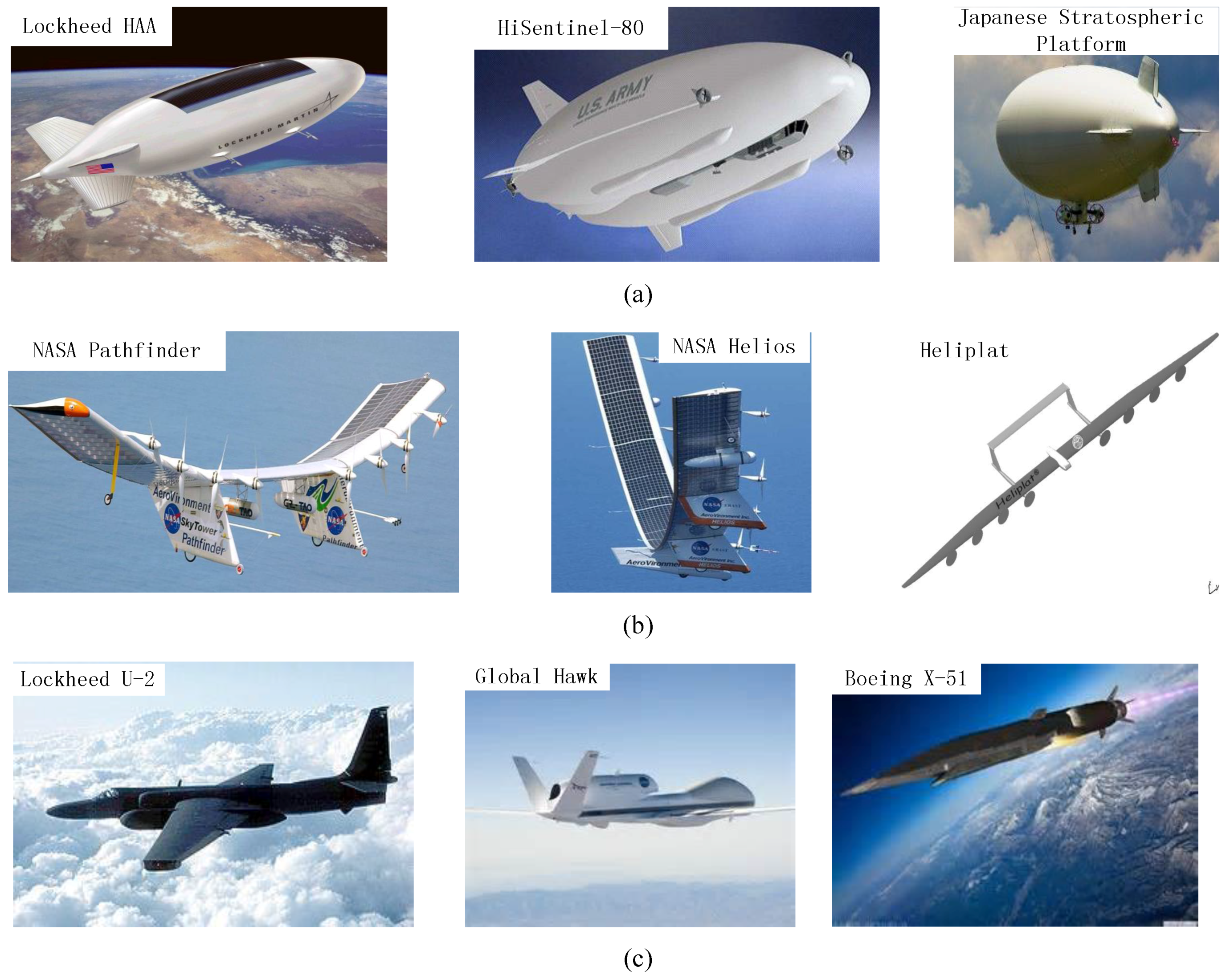
:1. Introduction
2. NS-TOPSAR
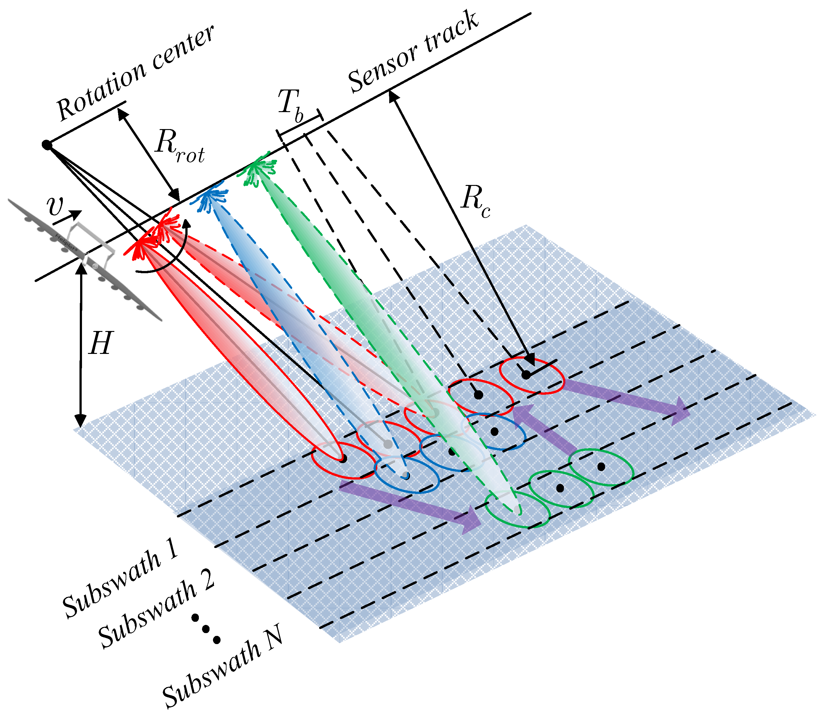
2.1. Geometry Model and Echo Signal Model
2.2. Echo Signal Property
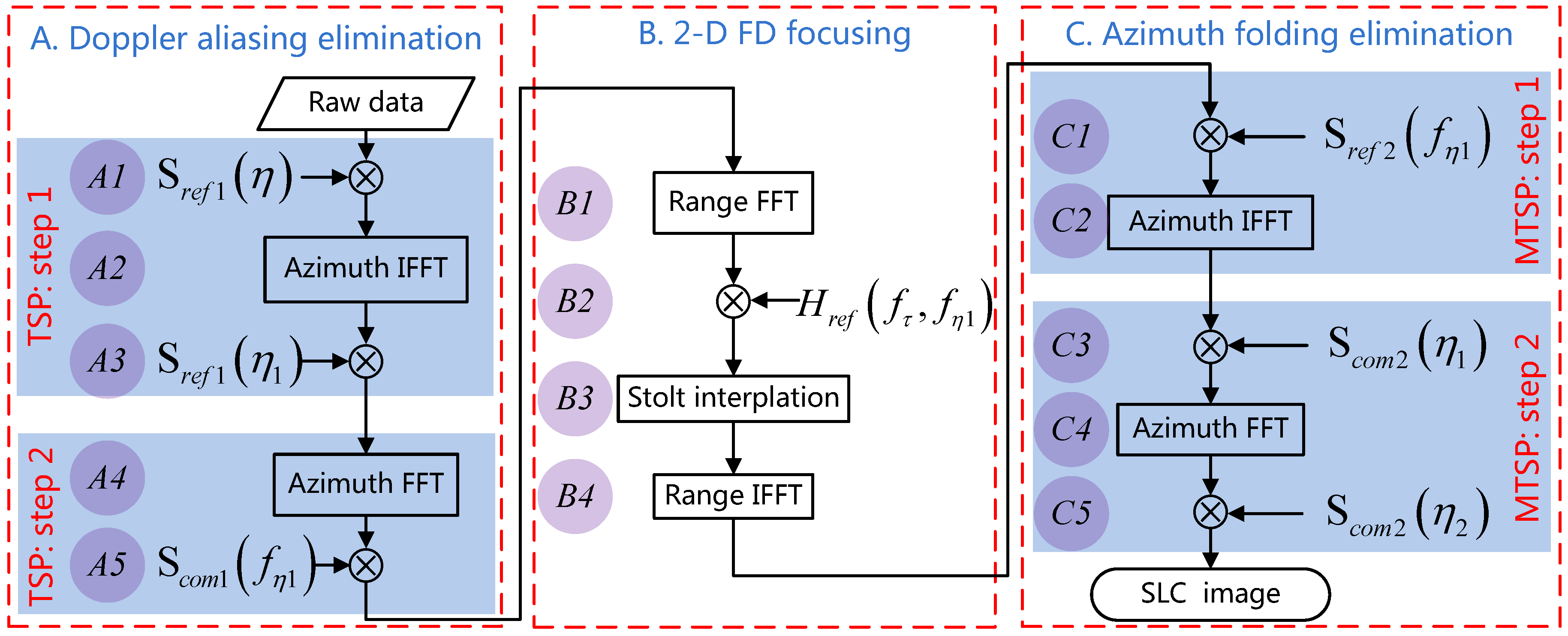
3. Imaging Scheme
3.1. Doppler Aliasing Elimination by TSP
3.2. 2D FD Focusing by
3.3. Azimuth Folding Elimination by MTSP
4. Simulation
4.1. Simulation Parameters
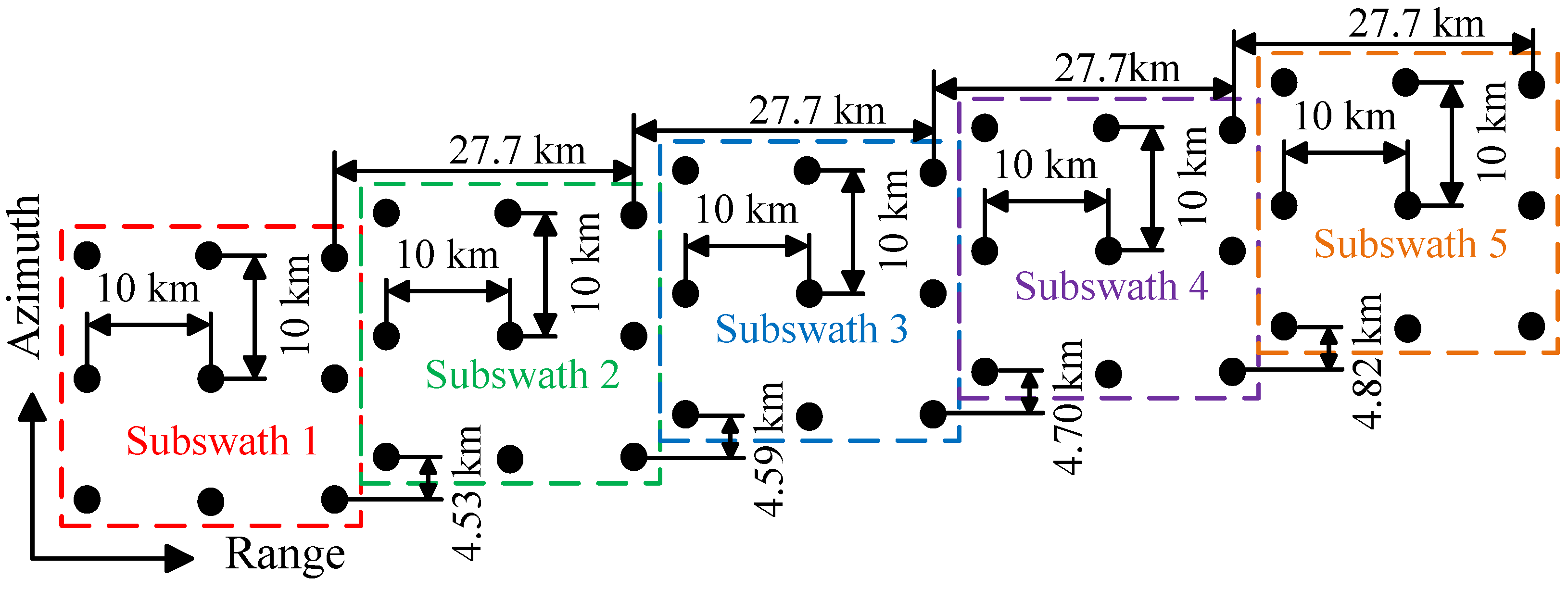
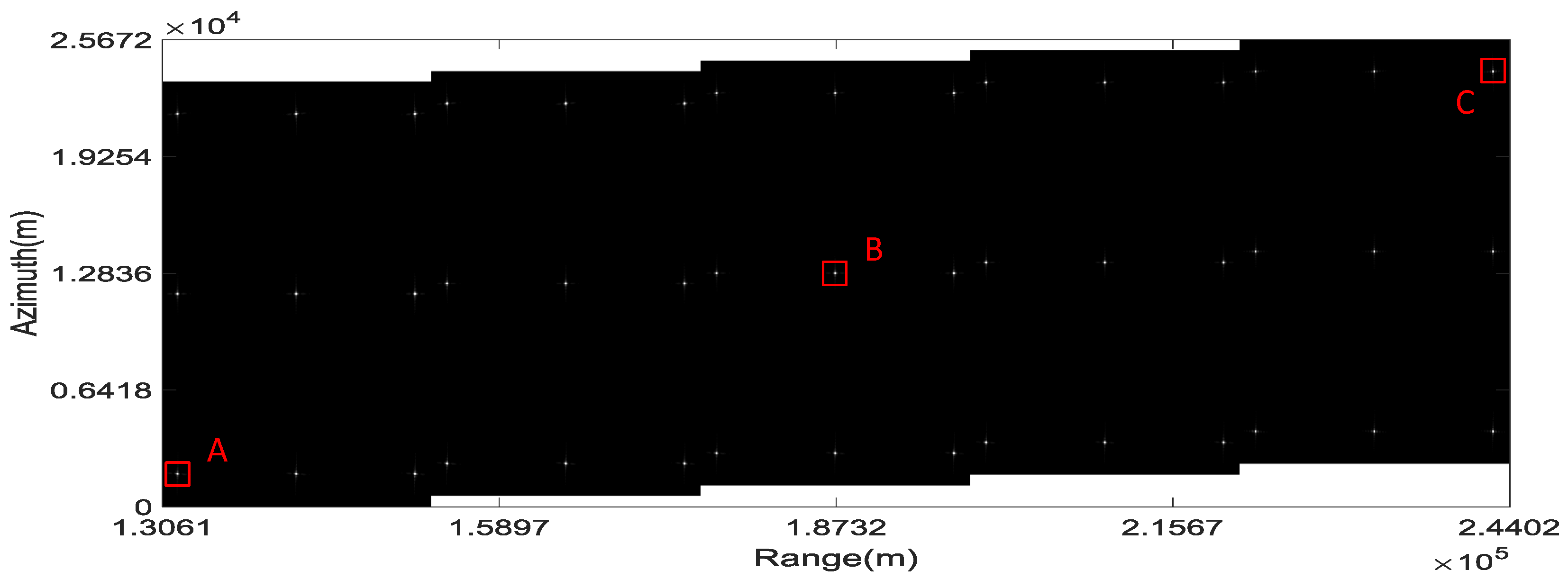
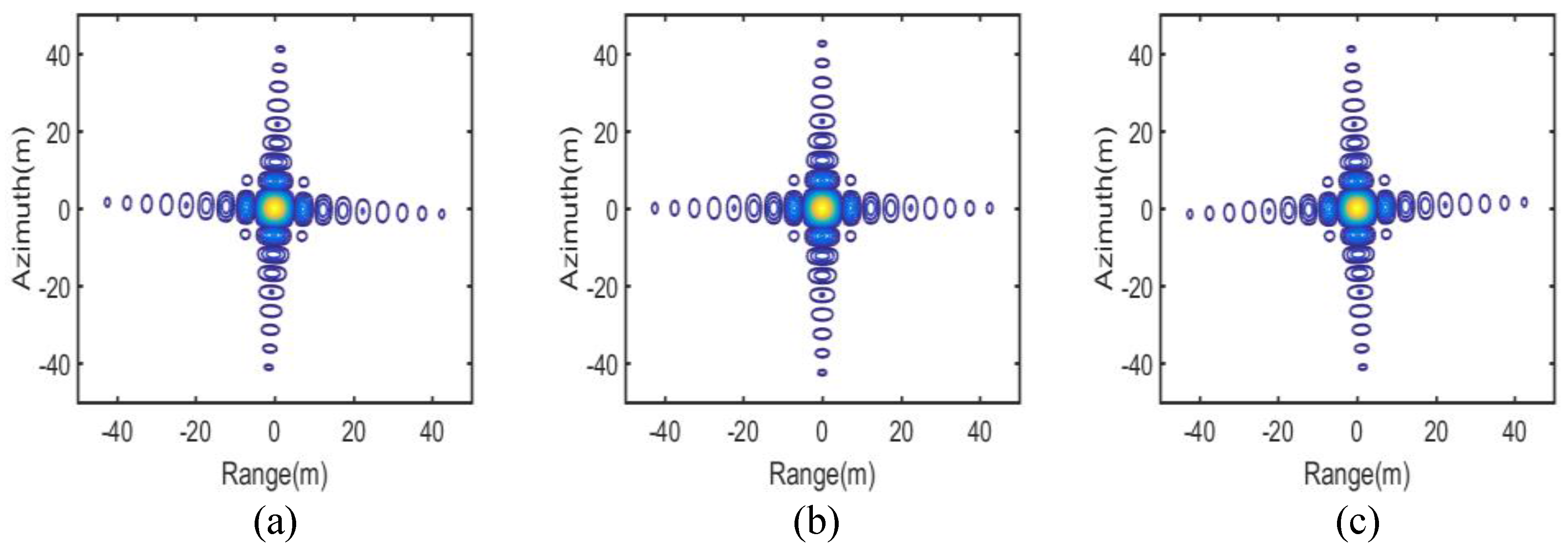
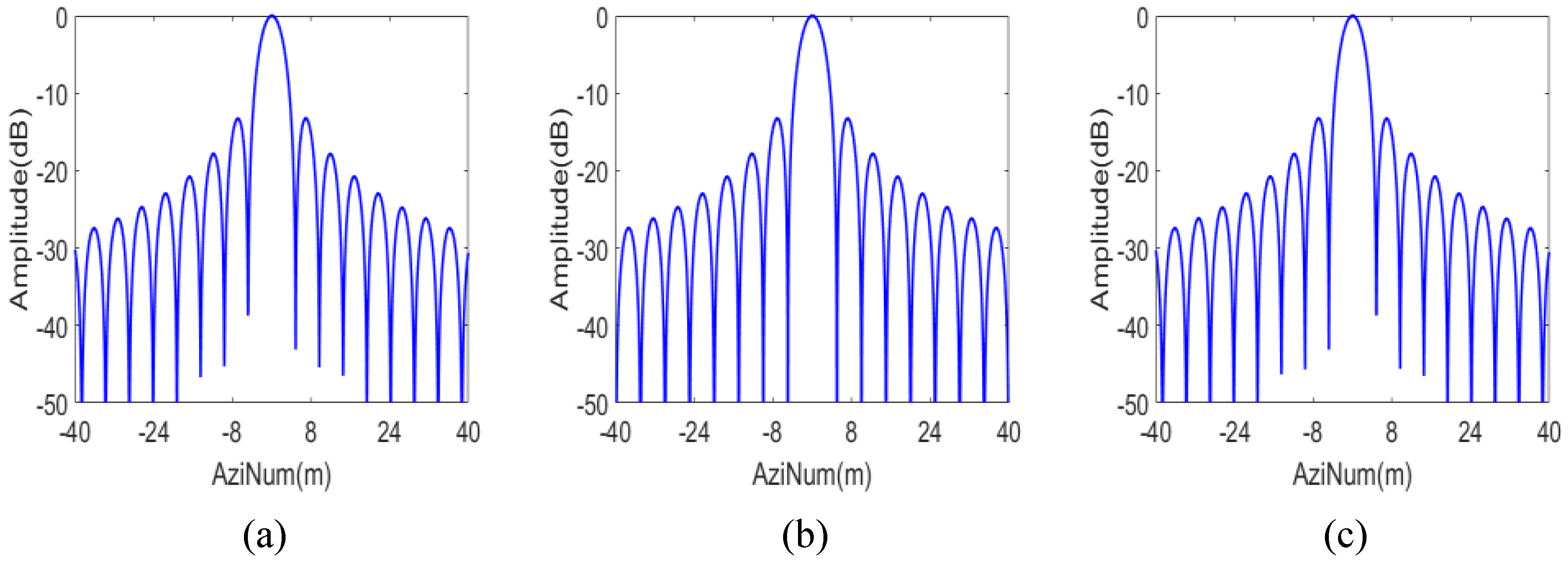
4.2. Simulation Results
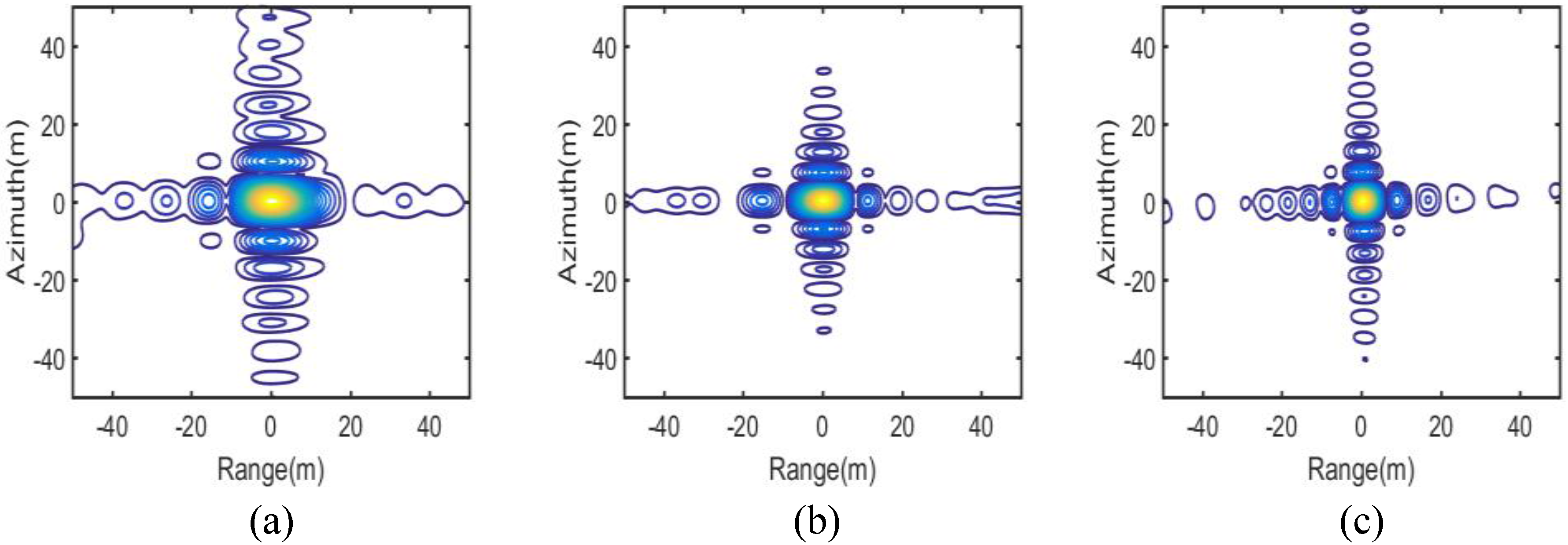
4.3. Imaging Scheme Comparison and Discussion
4.4. Performance Comparison of NS-TOPSAR and Spaceborne/Airborne TOPSAR
5. Conclusions
Acknowledgments
Author Contributions
Conflicts of Interest
References
- Allen, E.H. The case for near space. Aerosp. Am. 2006, 44, 31–34. [Google Scholar]
- Wang, W.Q. Near-space vehicles: Supply a gap between satellites and airplanes for remote sensing. IEEE Aerosp. Electron. Syst. Mag. 2011, 26, 4–9. [Google Scholar] [CrossRef]
- Wang, W.Q. Near-space vehicle-borne SAR with reflector antenna for high-resolution and wide-swath remote sensing. IEEE Trans. Geosci. Remote Sens. 2012, 50, 338–348. [Google Scholar] [CrossRef]
- Wang, W.Q.; Jiang, D. Integrated wireless sensor systems via near-space and satellite platforms: A review. IEEE Sens. J. 2014, 14, 3903–3914. [Google Scholar] [CrossRef]
- Wang, W.Q. Near-space wide-swath radar imaging with multiaperture antenna. IEEE Antennas Wirel. Propag. Lett. 2009, 8, 461–464. [Google Scholar] [CrossRef]
- Wang, W.Q. Large-area remote sensing in high-altitude high-speed platform using MIMO SAR. IEEE J. Sel. Top. Appl. Earth Observ. Remote Sens. 2013, 6, 2146–2158. [Google Scholar] [CrossRef]
- Wang, W.Q.; Shao, H. High altitude platform multichannel SAR for wide-area and staring imaging. IEEE Aerosp. Electron. Syst. Mag. 2014, 29, 12–17. [Google Scholar]
- Hank, J.M.; Murphy, J.S.; Mutzman, R.C. The X-51A scramjet engine flight demonstration program. In Proceedings of the 15th AIAA International Space Planes and Hypersonic Systems and Technologies Conference, Dayton, OH, USA, 28 April–1 May 2008. [CrossRef]
- Rigling, B.; Garber, W.; Hawley, R.; Gorham, L. Wide-area, persistent SAR imaging: Algorithm tradeoffs. IEEE Aerosp. Electron. Syst. Mag. 2014, 29, 14–20. [Google Scholar] [CrossRef]
- Gebert, N.; Krieger, G.; Moreira, A. Digital beamforming on receive: Techniques and optimization strategies for high-resolution wide-swath SAR imaging. IEEE Trans. Aerosp. Electron. Syst. 2009, 45, 564–592. [Google Scholar] [CrossRef]
- Dickinson, R.M. Power in the sky: Requirements for microwave wireless power beamers for powering high-altitude platforms. IEEE Microw. Mag. 2013, 14, 36–47. [Google Scholar] [CrossRef]
- Romeo, G.; Frulla, G. HELIPLAT®: High altitude very-long endurance solar powered UAV for telecommunication and Earth observation applications. Aeronaut. J. 2004, 108, 277–293. [Google Scholar] [CrossRef]
- Frulla, G. Aeroelastic behaviour of a solar-powered high-altitude long endurance unmanned air vehicle (HALE-UAV) slender wing. Proc. Inst. Mech. Eng. Part G J. Aerosp. Eng. 2004, 218, 179–188. [Google Scholar] [CrossRef]
- Kennedy, J.F. Balloons in Today’s Military? Air Space Power J. 2005, 19, 39–49. [Google Scholar]
- Wang, W.Q. Distributed passive radar sensor networks with near-space vehicle-borne receivers. Wirel. Sens. Syst. IET 2012, 2, 183–190. [Google Scholar] [CrossRef]
- Tozer, T.; Grace, D. High-altitude platforms for wireless communications. Electron. Commun. Eng. J. 2001, 13, 127–137. [Google Scholar] [CrossRef]
- Mohammed, A.; Mehmood, A.; Pavlidou, F.N.; Mohorcic, M. The role of high-altitude platforms (HAPs) in the global wireless connectivity. Proc. IEEE 2011, 99, 1939–1953. [Google Scholar] [CrossRef]
- De Zan, F.; Guarnieri, A.M. TOPSAR: Terrain observation by progressive scans. IEEE Trans. Geosci. Remote Sens. 2006, 44, 2352–2360. [Google Scholar] [CrossRef]
- Li, W.; Yang, J.; Huang, Y.; Yang, H.; Zhang, Q.; Liu, Z.; Wu, J. Signal properties of tops-based near space slow-speed SAR. In Proceedings of the IGARSS, Melbourne, Australia, 21–26 July 2013; pp. 1333–1335.
- Prats, P.; Scheiber, R.; Mittermayer, J.; Meta, A.; Moreira, A. Processing of sliding spotlight and TOPS SAR data using baseband azimuth scaling. IEEE Trans. Geosci. Remote Sens. 2010, 48, 770–780. [Google Scholar] [CrossRef]
- Engen, G.; Larsen, Y. Efficient full aperture processing of TOPS mode data using the moving band CZT. IEEE Trans. Geosci. Remote Sens. 2011, 49, 3688–3693. [Google Scholar] [CrossRef]
- Sun, G.C.; Xing, M.; Xia, X.G.; Wu, Y.; Bao, Z. Beam steering SAR data processing by a generalized PFA. IEEE Trans. Geosci. Remote Sens. 2013, 51, 4366–4377. [Google Scholar] [CrossRef]
- Mao, X.; Zhu, D.; Zhu, Z. Polar format algorithm wavefront curvature compensation under arbitrary radar flight path. IEEE Geosci. Remote Sens. Lett. 2012, 9, 526–530. [Google Scholar] [CrossRef]
- Sun, G.; Xing, M.; Wang, Y.; Wu, Y.; Wu, Y.; Bao, Z. Sliding spotlight and TOPS SAR data processing without subaperture. IEEE Geosci. Remote Sens. Lett. 2011, 8, 1036–1040. [Google Scholar] [CrossRef]
- Lanari, R.; Tesauro, M.; Sansosti, E.; Fornaro, G. Spotlight SAR data focusing based on a two-step processing approach. IEEE Trans. Geosci. Remote Sens. 2001, 39, 1993–2004. [Google Scholar] [CrossRef]
- Sack, M.; Ito, M.; Cumming, I. Application of efficient linear FM matched filtering algorithms to synthetic aperture radar processing. Commun. Radar Signal Process. 1985, 132, 45–57. [Google Scholar] [CrossRef]
- Xu, W.; Huang, P.; Wang, R.; Deng, Y.; Lu, Y. TOPS-mode raw data processing using chirp scaling algorithm. IEEE J. Sel. Top. Appl. Earth Observ. Remote Sens. 2014, 7, 235–246. [Google Scholar] [CrossRef]
- Xu, W.; Huang, P.; Deng, Y.; Sun, J.; Shang, X. An efficient approach with scaling factors for TOPS-mode SAR data focusing. IEEE J. Sel. Top. Appl. Earth Observ. Remote Sens. 2011, 8, 929–933. [Google Scholar] [CrossRef]
- Cafforio, C.; Prati, C.; Rocca, F. SAR data focusing using seismic migration techniques. IEEE Trans. Aerosp. Electron. Syst. 1991, 27, 194–207. [Google Scholar] [CrossRef]
- Berger, M.; Moreno, J.; Johannessen, J.A.; Levelt, P.F.; Hanssen, R.F. ESA’s sentinel missions in support of Earth system science. Remote Sens. Environ. 2012, 120, 84–90. [Google Scholar] [CrossRef]
- Torres, R.; Snoeij, P.; Geudtner, D.; Bibby, D.; Davidson, M.; Attema, E.; Potin, P.; Rommen, B.; Floury, N.; Brown, M.; et al. GMES Sentinel-1 mission. Remote Sens. Environ. 2012, 120, 9–24. [Google Scholar] [CrossRef]
- Malenovsky, Z.; Rott, H.; Cihlar, J.; Schaepman, M.E.; Garcia-Santos, G.; Fernandes, R.; Berger, M. Sentinels for science: Potential of Sentinel-1,-2, and-3 missions for scientific observations of ocean, cryosphere, and land. Remote Sens. Environ. 2012, 120, 91–101. [Google Scholar] [CrossRef]


| General Parameters | Value | ||||
|---|---|---|---|---|---|
| Carrier frequency (GHz) | 9 | ||||
| Chirp bandwidth (MHz) | 30 | ||||
| Chirp duration (s) | 2 | ||||
| Sample frequency (MHz) | 36 | ||||
| Antenna azimuth aperture (m) | 1.7 | ||||
| Platform velocity (m/s) | 20 | ||||
| Platform altitude (km) | 25 | ||||
| Number of subswath | 5 | ||||
| Total swath width (km) | 115 | ||||
| TOPS coefficient | 5.2 | ||||
| Swath-dependent parameters | Subswath | ||||
| 1 | 2 | 3 | 4 | 5 | |
| Slant range of center (km) | 97 | 142 | 187 | 233 | 278 |
| PRF (Hz) | 113 | 60 | 41 | 32 | 27 |
| Total Doppler bandwidth (Hz) | 267 | 178 | 136 | 112 | 96 |
| Target | 3 dB IRW (dB) | PSLR (dB) | ISLR (dB) |
|---|---|---|---|
| A | 4.439 | -13.262 | -9.852 |
| B | 4.432 | -13.266 | -9.882 |
| C | 4.438 | -13.264 | -9.854 |
| D | 6.161 | -12.558 | -2.788 |
| E | 4.436 | -13.092 | -10.202 |
| F | 4.638 | -13.164 | -9.982 |
| NS-TOPSAR | Sentinel-1 | Airborne | ||
|---|---|---|---|---|
| IW Mode | EW Mode | TOPSAR in [24] | ||
| Carrier frequency (GHz) | 9 | 5.405 | 5.405 | 9.65 |
| Altitude (km) | 25 | 693 | 693 | 5 |
| Resolution | 4.5 × 4.5 | 5 × 20 | 20 × 40 | 2 × 1 |
| (range × azimuth, m) | ||||
| Swathwidth (km) | 100 | 250 | 400 | 20 |
| Revisit time | several hours | 6 days | 6 days | within one hour |
| Endurance | up to a few years | tens of years | tens of years | up to a few days |
© 2016 by the authors; licensee MDPI, Basel, Switzerland. This article is an open access article distributed under the terms and conditions of the Creative Commons Attribution (CC-BY) license (http://creativecommons.org/licenses/by/4.0/).
Share and Cite
Zhang, Q.; Wu, J.; Li, W.; Huang, Y.; Yang, J.; Yang, H. Near-Space TOPSAR Large-Scene Full-Aperture Imaging Scheme Based on Two-Step Processing. Sensors 2016, 16, 1177. https://doi.org/10.3390/s16081177
Zhang Q, Wu J, Li W, Huang Y, Yang J, Yang H. Near-Space TOPSAR Large-Scene Full-Aperture Imaging Scheme Based on Two-Step Processing. Sensors. 2016; 16(8):1177. https://doi.org/10.3390/s16081177
Chicago/Turabian StyleZhang, Qianghui, Junjie Wu, Wenchao Li, Yulin Huang, Jianyu Yang, and Haiguang Yang. 2016. "Near-Space TOPSAR Large-Scene Full-Aperture Imaging Scheme Based on Two-Step Processing" Sensors 16, no. 8: 1177. https://doi.org/10.3390/s16081177
APA StyleZhang, Q., Wu, J., Li, W., Huang, Y., Yang, J., & Yang, H. (2016). Near-Space TOPSAR Large-Scene Full-Aperture Imaging Scheme Based on Two-Step Processing. Sensors, 16(8), 1177. https://doi.org/10.3390/s16081177