
Underdetermined Blind Source Separation with Variational Mode Decomposition for Compound Roller Bearing Fault Signals


Abstract
:1. Introduction
2. Underdetermined Blind Source Separation
- (1)
- source signals are statistically independent of each other;
- (2)
- hybrid matrix is a matrix with full column rank;
- (3)
- noise signals are statistically independent of each other and are irrelevant to the original signals.
- (4)
- The number of source signals () is less than or equal to the number of observed signals ().
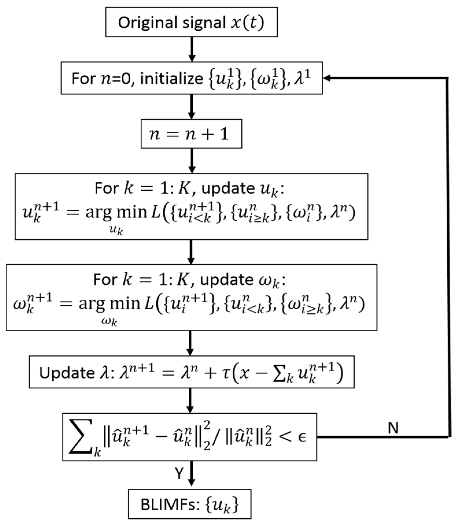
3. Variational Mode Decomposition
4. Independent Component Analysis
- Step 1.
- Step 2.
- Step 3.
- Step 4.
- Step 5.
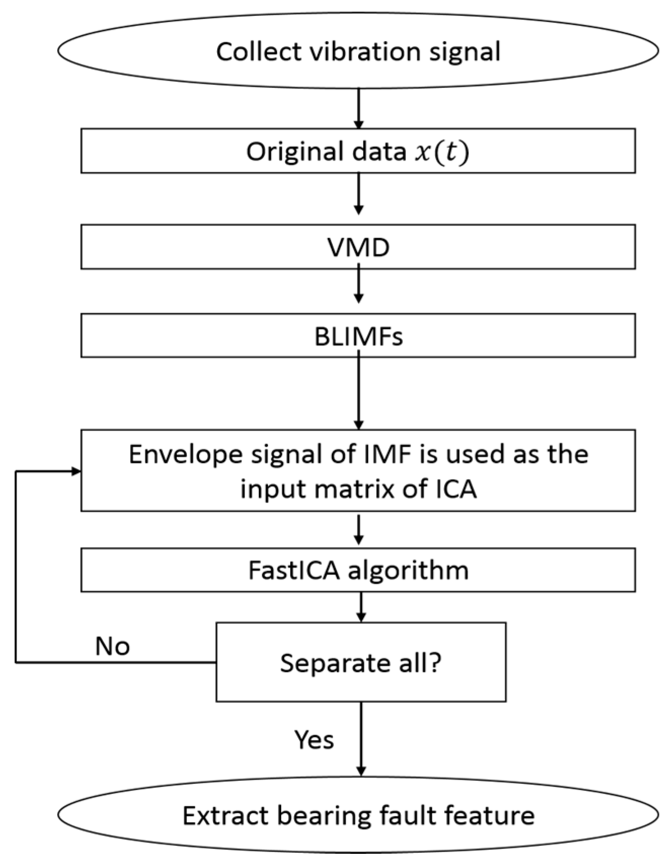
5. Proposed Method
6. Experimental Results
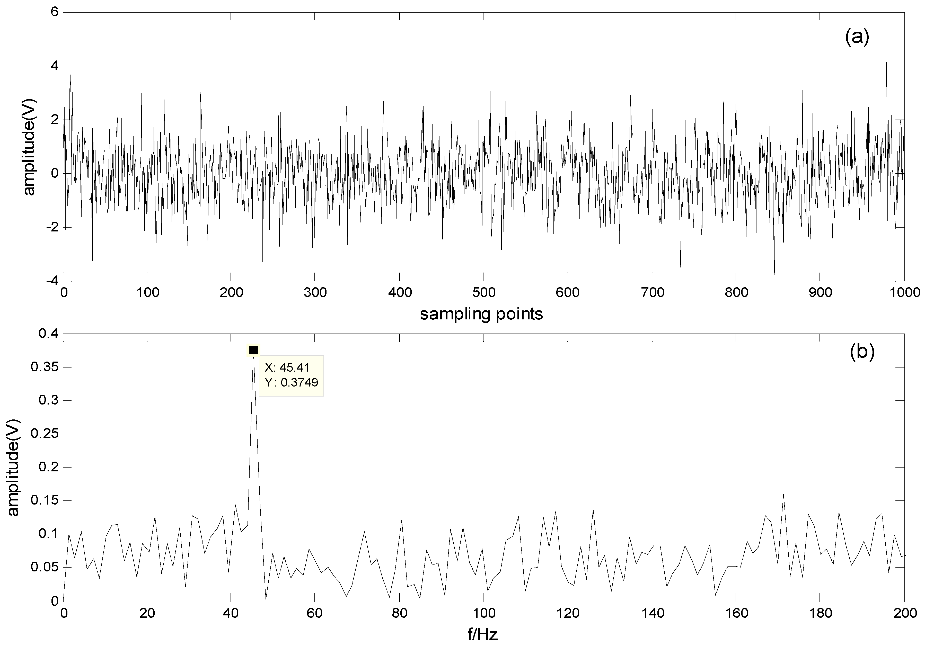
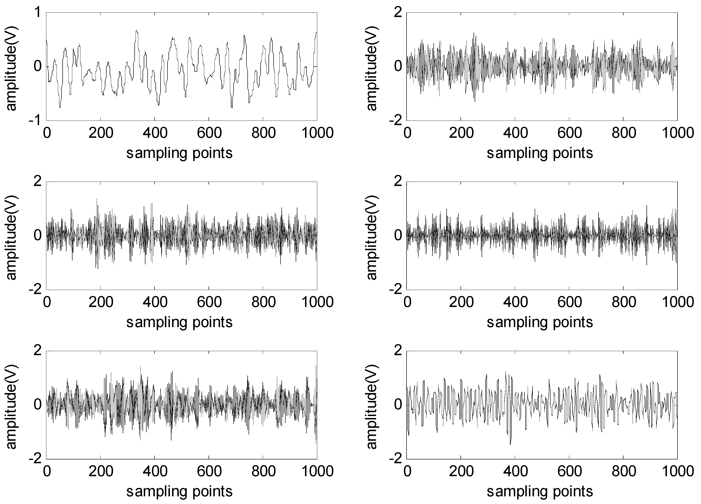
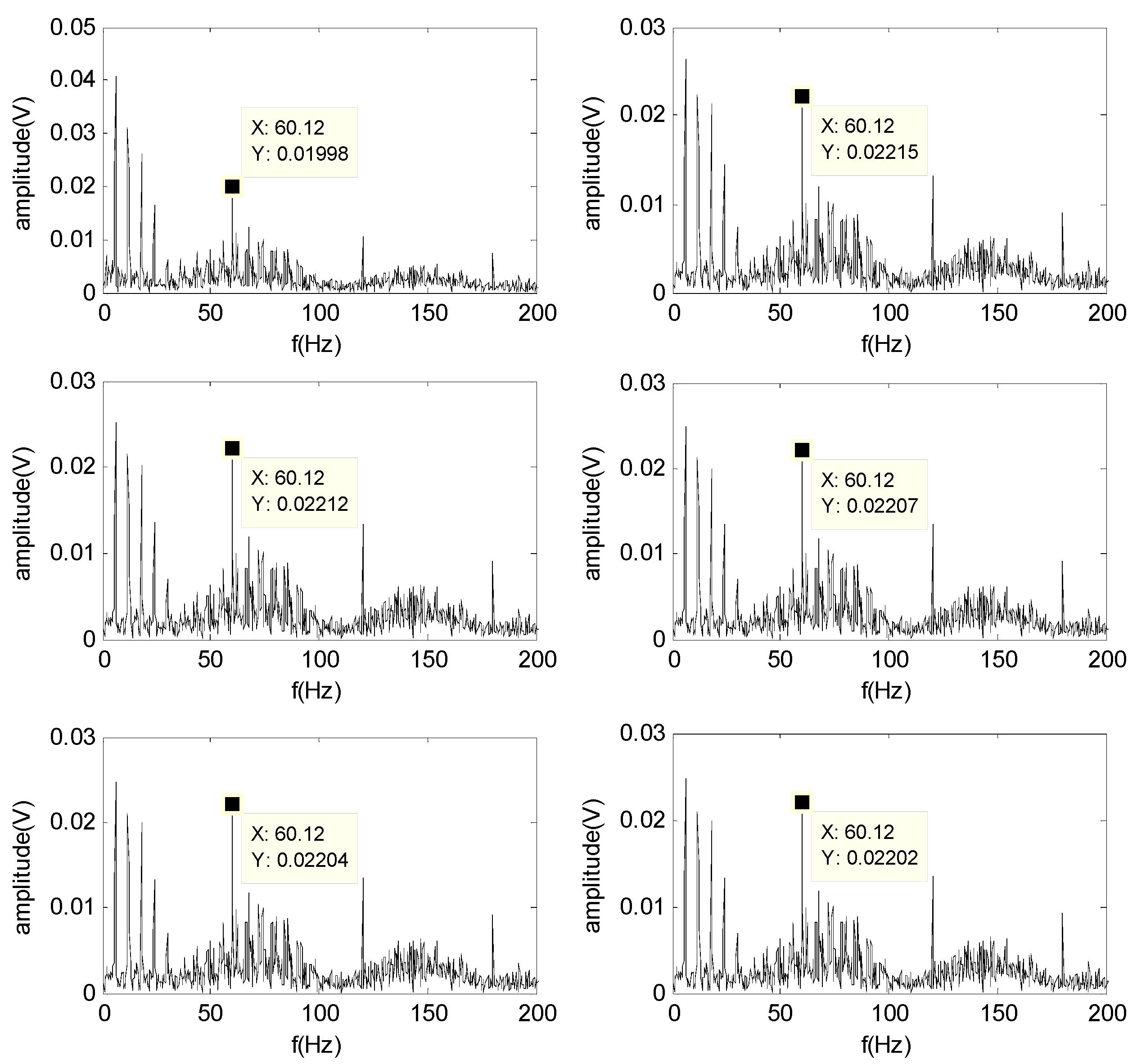
6.1. Simulation
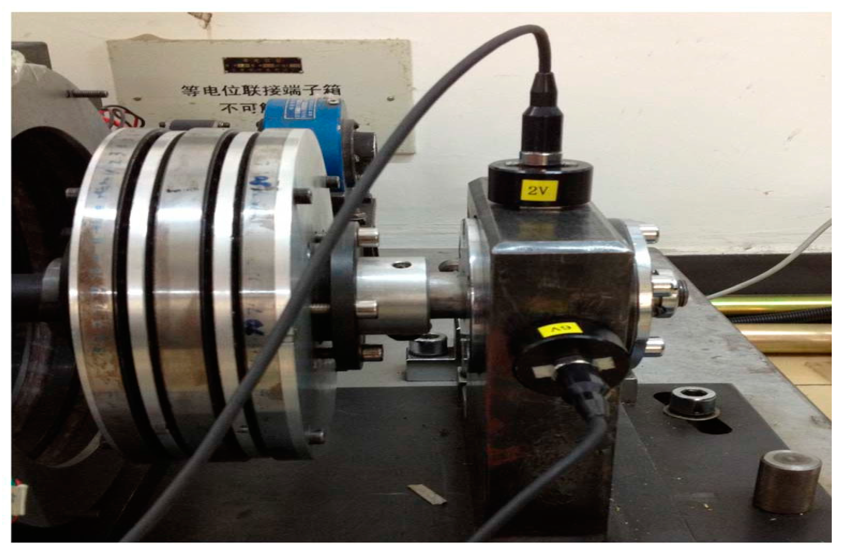
6.2. Experimental Setup
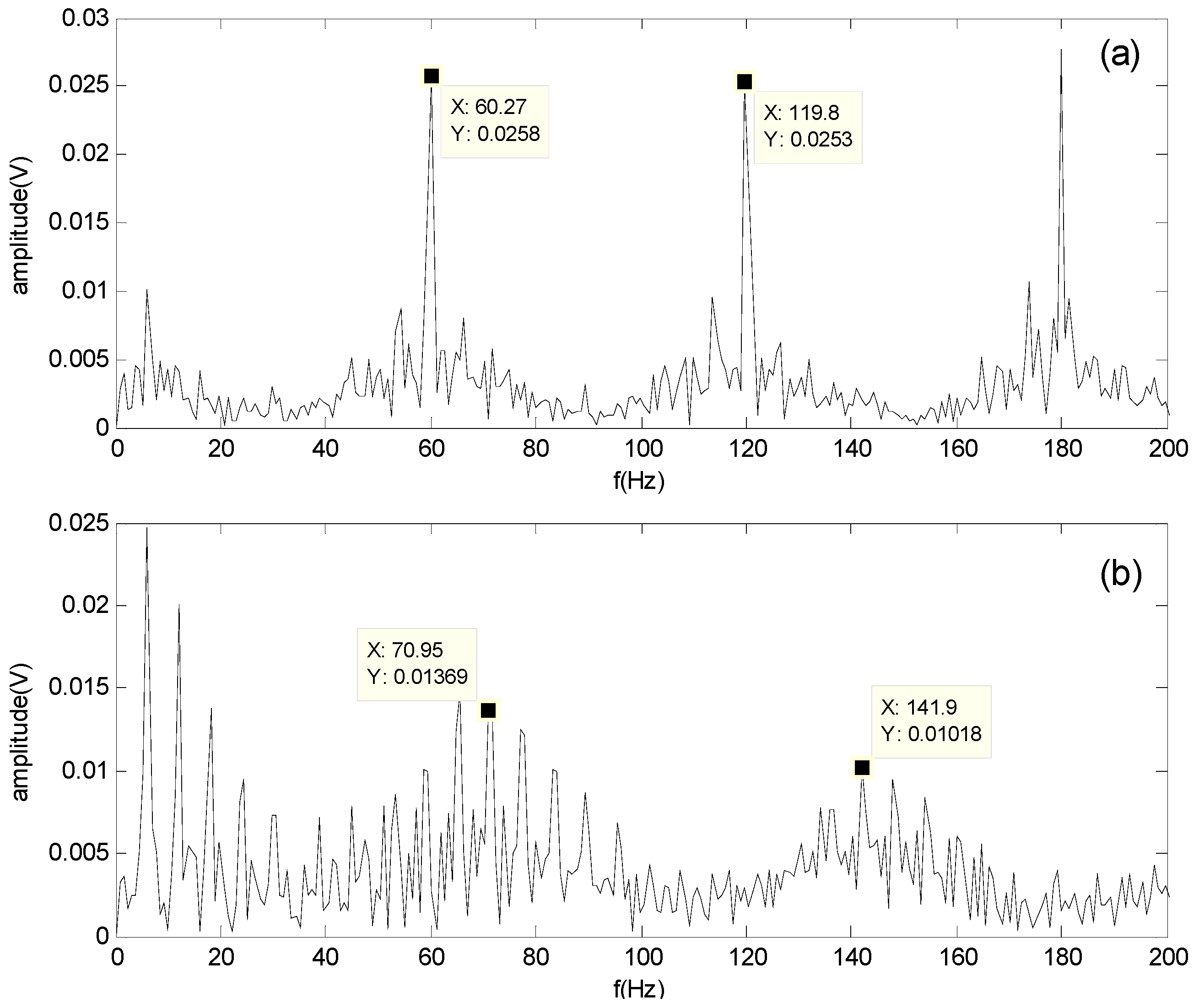
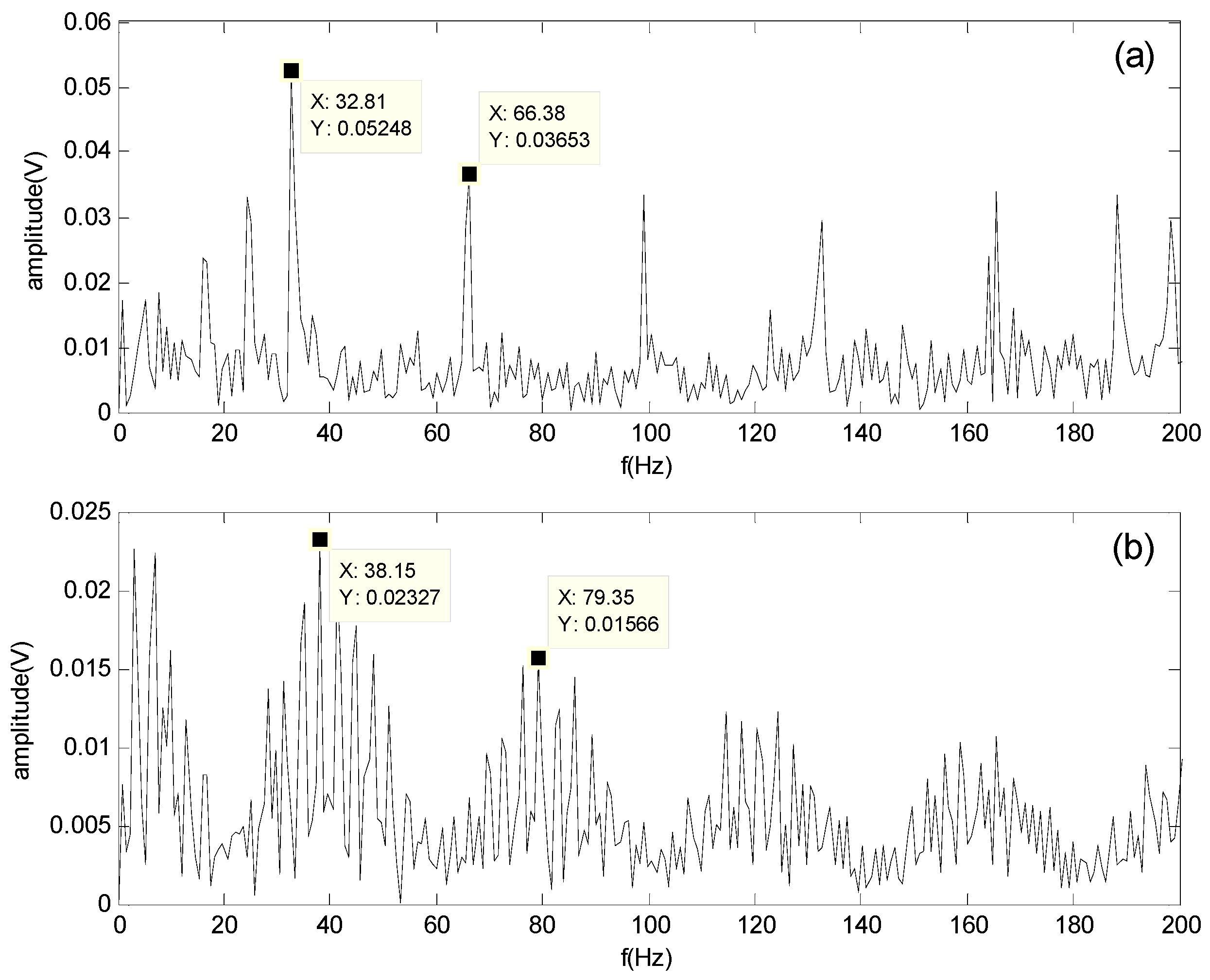
6.3. Diagnosis by Traditional Envelope Spectrum Analysis
- (1)
- The theoretical frequency is calculated based on the assumption of a pure rolling motion. However, in practice, some sliding motion may occur.
- (2)
- In practice, some installation error will appear in the roller bearing.
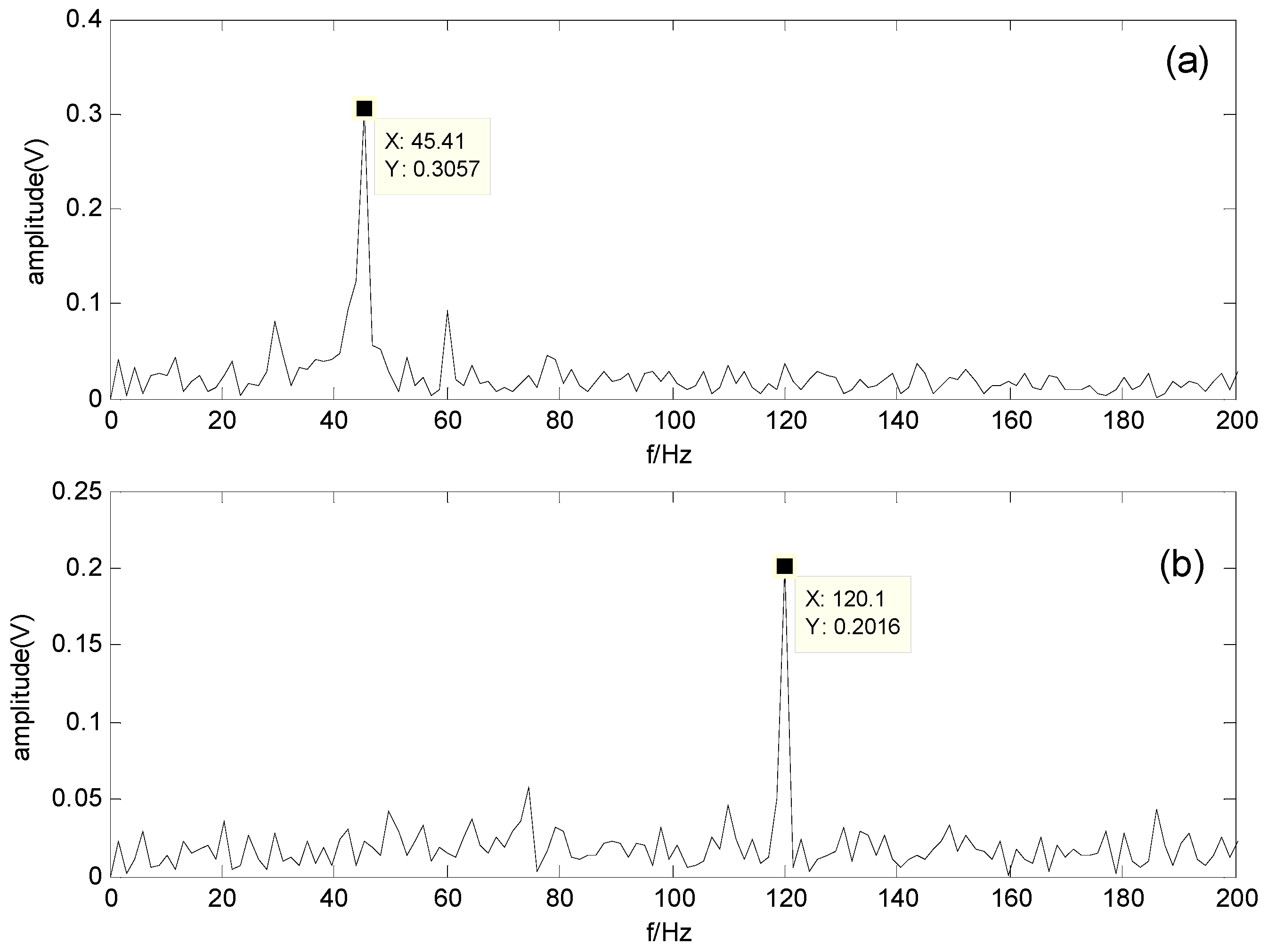
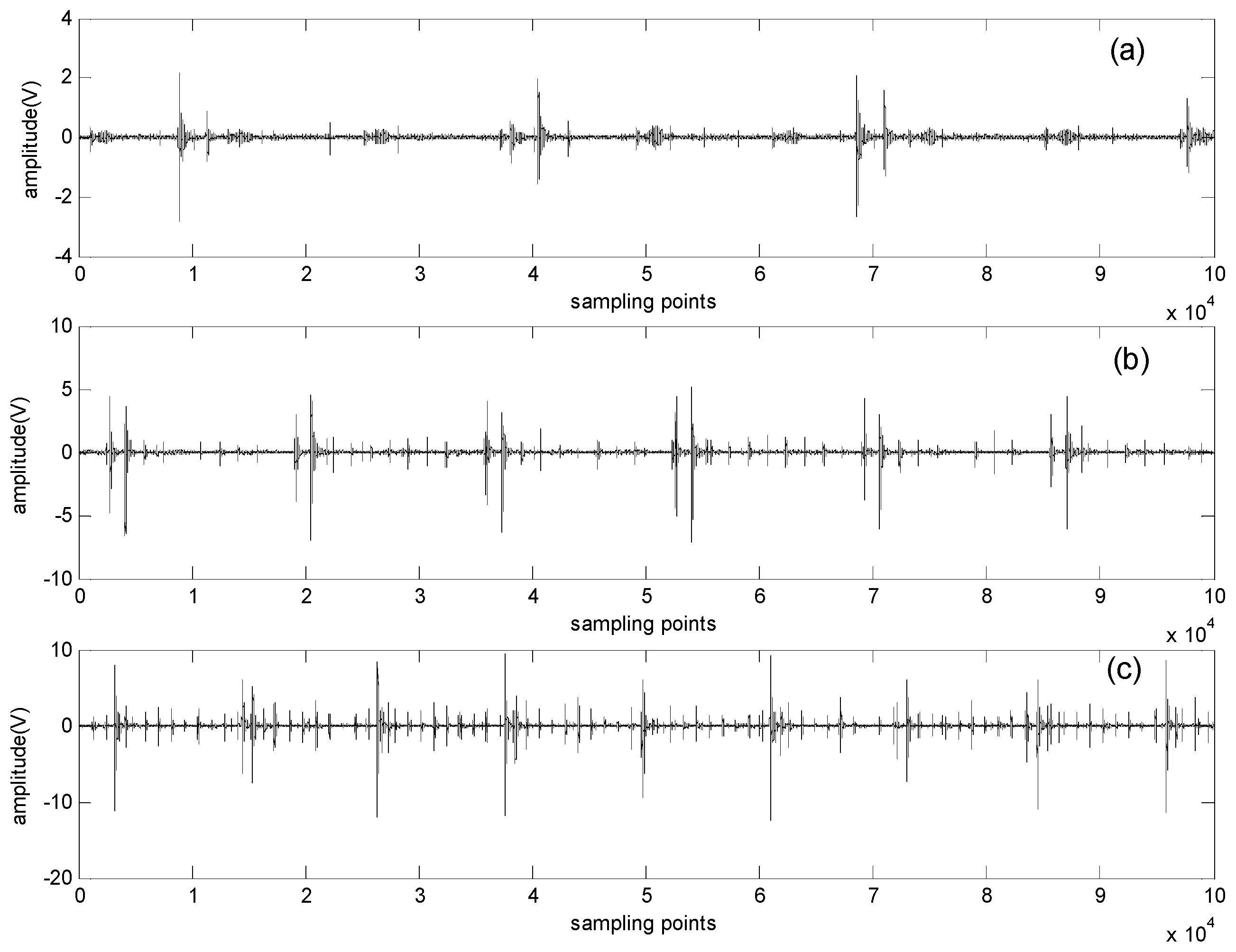
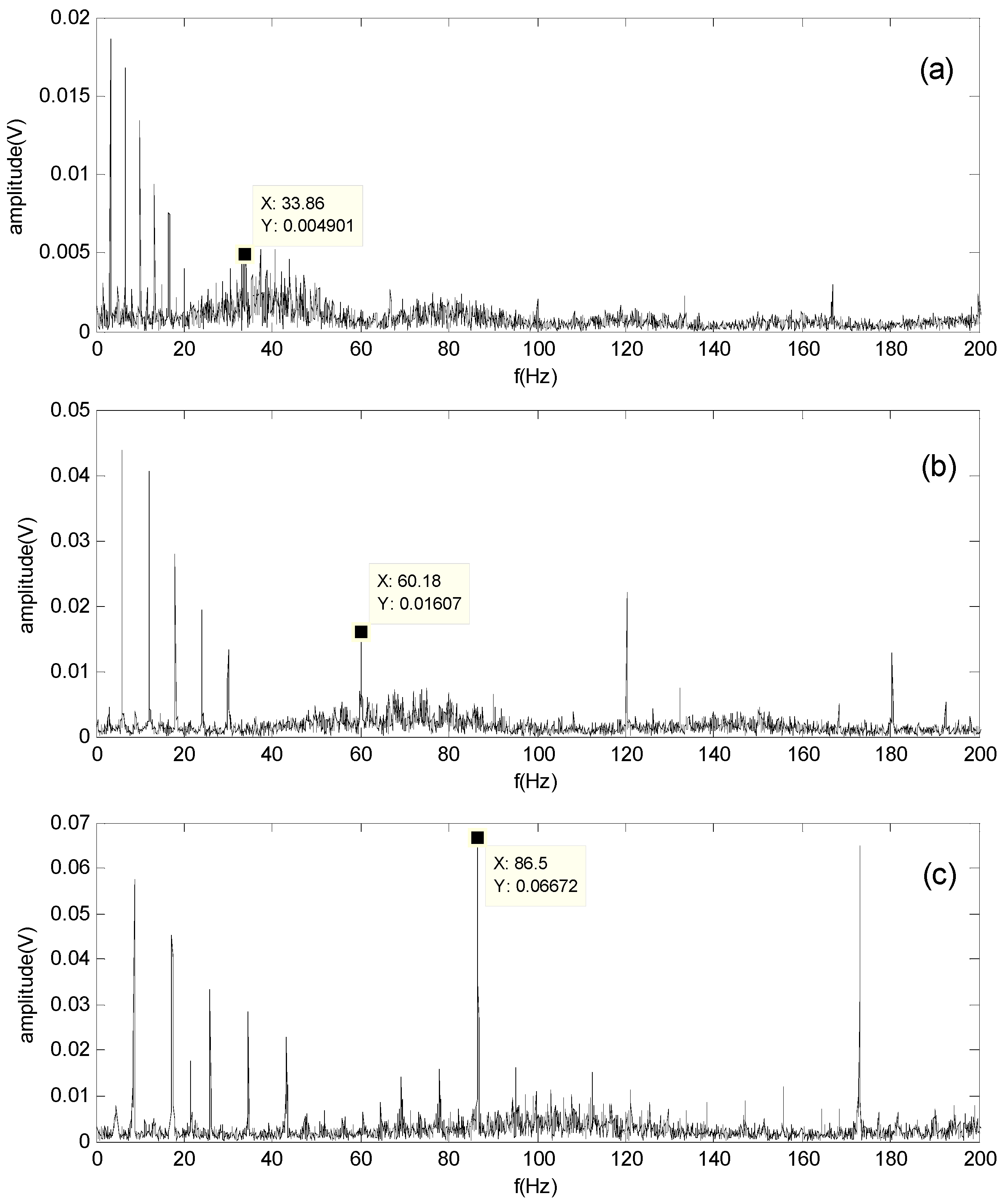
6.4. Diagnosis by the Proposed Method
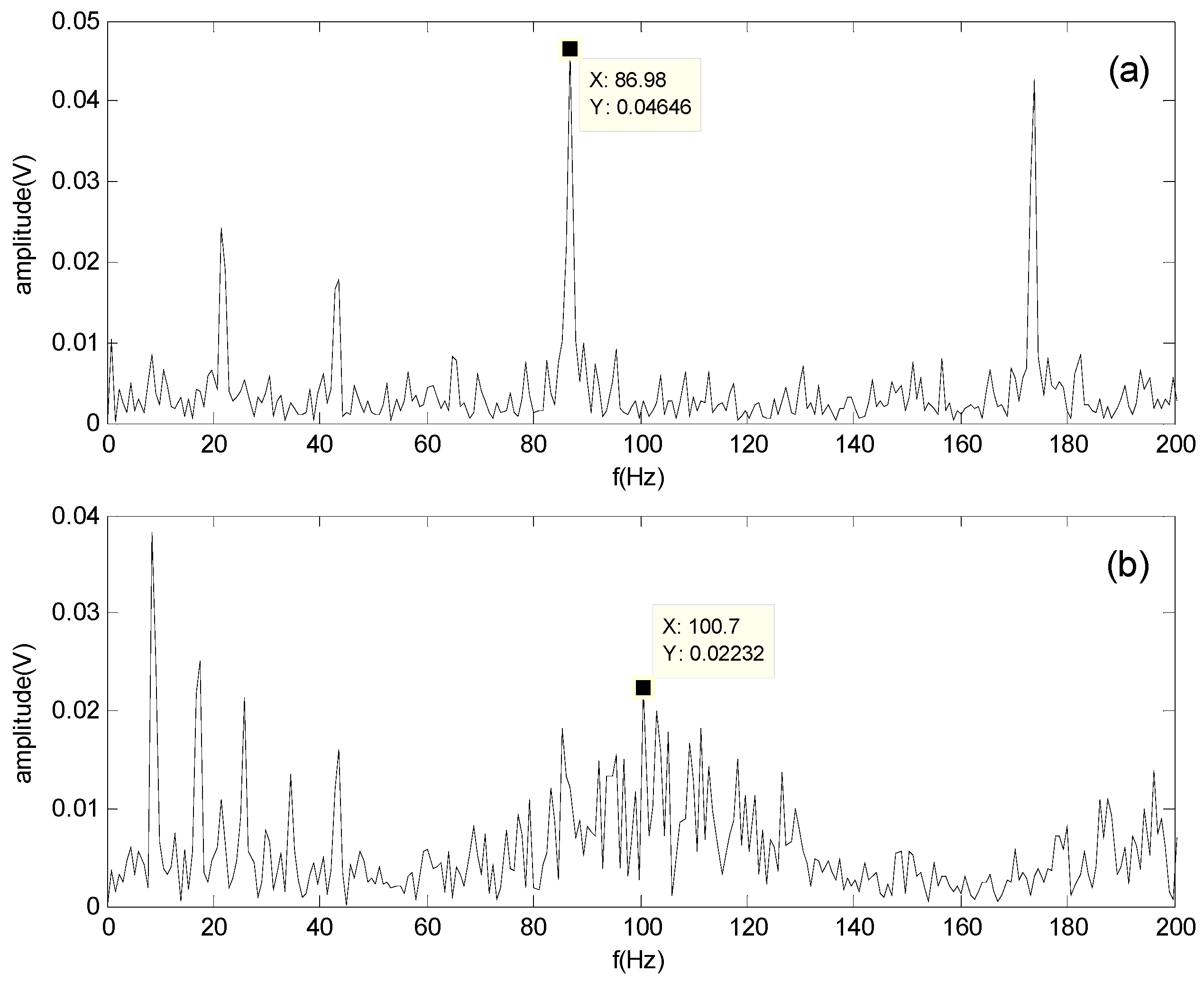
6.5. Comparison of the Proposed Method with the EEMD Method
7. Conclusions
Acknowledgments
Author Contributions
Conflicts of Interest
References
- Harris, T. Rolling Bearing Analysis; John Wiley and Sons, Inc.: Malden, MA, USA, 1991. [Google Scholar]
- Wang, Y.; Kang, S.; Jiang, Y.; Yang, G.; Song, L.; Mikulovich, V.I. Classification of fault location and the degree of performance degradation of a rolling bearing based on an improved hyper-sphere-structured multi-class support vector machine Mech. Syst. Signal Process. 2012, 29, 404–414. [Google Scholar] [CrossRef]
- Rajagopalan, S.; Restrepo, J.; Aller, J.M.; Habetler, T.G.; Harley, R.G. Nonstationary motor fault detection using recent quadratic time-Frequency representations. IEEE Trans. Ind. Appl. 2008, 44, 735–744. [Google Scholar] [CrossRef]
- Zhang, P.; Du, Y.; Habetler, T.G.; Lu, B. A survey of condition monitoring and protection methods for medium-voltage induction motors. IEEE Trans. Ind. Appl. 2011, 47, 34–46. [Google Scholar] [CrossRef]
- Riera-Guasp, M.; Antonino, D.J.; Roger, F.J.; Palomares, M. The use of the wavelet approximation signal as a tool for the diagnosis of rotor bar failures. IEEE Trans. Ind. Appl. 2008, 44, 716–726. [Google Scholar] [CrossRef]
- Al-Ahmar, E.; Benbouzid, M.; Turri, S. Wind energy conversion systems fault diagnosis using wavelet analysis. Int. Rev. Electr. Eng. 2008, 3, 646–652. [Google Scholar]
- Zarzoso, V.; Nandi, A.K. Blind source separation. In Blind Estimation Using Higher-Order Statistics; Springer: New Tork, NY, USA, 1999; pp. 167–252. [Google Scholar]
- Hyvärinen, A.; Karhunen, J.; Oja, E. Independent Component Analysis; John Wiley & Sons: Malden, MA, USA, 2004. [Google Scholar]
- Mallat, S.G. A theory for multiresolution signal decomposition: The wavelet representation. IEEE Trans. Pattern Anal. Mach. Intell. 1989, 11, 674–693. [Google Scholar] [CrossRef]
- Chen, B.; Chen, X.; He, Z.; Tan, J. Mechanical fault diagnosis based on local mean decomposition method. In Proceedings of the International Conference on Measuring Technology and Mechatronics Automation, Zhangjiajie, China, 11–12 April 2009; Volume 1, pp. 681–684.
- Rilling, G.; Flandrin, P.; Goncalves, P. On empirical mode decomposition and its algorithms. In Proceedings of the IEEE-EURASIP Workshop Nonlinear Signal and Image Processing, Grado, Italy, 6 June 2003; Volume 3, pp. 8–11.
- Huang, N.E. Hilbert-Huang Transform and Its Applications; World Scientific: Singapore, 2014. [Google Scholar]
- Yang, Q.; An, D. EMD and wavelet transform based fault diagnosis for wind turbine gear box. Adv. Mech. Eng. 2013, 5, 212836. [Google Scholar] [CrossRef]
- Shao, R.; Hu, W.; Li, J. Multi-fault feature extraction and diagnosis of gear transmission system using time-frequency analysis and wavelet threshold de-noising based on EMD. Shock Vib. 2013, 20, 763–780. [Google Scholar] [CrossRef]
- Zhang, J.H.; Li, L.J.; Ma, W.P.; Li, Z.Y.; Liu, Y. Application of EMD-ICA to fault diagnosis of rolling bearings. Chin. J. Mech. Eng. 2013, 24, 1468–1472. [Google Scholar]
- Lou, W.; Shi, G.; Zhang, J. Research and application of ICA technique in fault diagnosis for equipments. In Proceedings of the IEEE International Conference on Intelligent Computing and Intelligent Systems, Shanghai, China, 20–22 November 2009; Volume 4, pp. 310–313.
- Zhu, W.; Zhou, J.; Xiao, J.; Xiao, H.; Li, C. An ICA-EMD feature extraction method and its application to vibration signals of hydroelectric generating units. Proc. CSEE 2013, 29, 95–101. [Google Scholar]
- Yang, Y.; Deng, J.; Wu, C. Analysis of mode mixing phenomenon in the empirical mode decomposition method. In Proceedings of the Second International Symposium on Information Science and Engineering, Shanghai, China, 26–28 December 2009; pp. 553–556.
- Ricci, R.; Pennacchi, P.; Lombardi, M.; Mirabile, C. Failure diagnostics of a spiral bevel gearbox using EMD and HHT. In Proceedings of the ISMA2010 including USD, Leuven, Belgium, 20–22 September 2010; pp. 20–22.
- Wu, Z.; Huang, N.E. Ensemble empirical mode decomposition: A noise-assisted data analysis method. Adv. Adapt. Data Anal. 2009, 1, 1–41. [Google Scholar] [CrossRef]
- Dragomiretskiy, K.; Zosso, D. Variational mode decomposition. IEEE Trans. Signal Proc. 2014, 62, 531–544. [Google Scholar] [CrossRef]
- Mohanty, S.; Gupta, K.K.; Raju, K.S. Bearing fault analysis using variational mode decomposition. J. Instrum. Technol. Innov. 2014, 42, 20–27. [Google Scholar]
- Mohanty, S.; Gupta, K.K.; Raju, K.S. Comparative study between VMD and EMD in bearing fault diagnosis. In Proceedings of the 9th International Conference on Industrial and Information Systems (ICIIS), Gwalior, India, 15–17 December 2014; pp. 1–6.
- Wang, H.; Li, R.; Tang, G.; Yuan, H.; Zhao, Q.; Cao, X. A compound fault diagnosis for rolling bearings method based on blind source separation and ensemble empirical mode decomposition. PLoS ONE 2014, 9, 1–13. [Google Scholar] [CrossRef] [PubMed]
- Liu, H.; Song, B.; Qin, H.; Qiu, Z. An adaptive-ADMM algorithm with support and signal value detection for compressed sensing. Signal Proc. Lett. 2013, 20, 315–318. [Google Scholar] [CrossRef]
- Hyvärinen, A.; Oja, E. A fast fixed-point algorithm for independent component analysis. Neural Comput. 1997, 9, 1483–1492. [Google Scholar] [CrossRef]
- Hyvärinen, A.; Pajunen, P. Nonlinear independent component analysis: Existence and uniqueness results. Neural Comput. 1999, 12, 429–439. [Google Scholar] [CrossRef]
- Hyvärinen, A.; Oja, E. Independent component analysis: Algorithms and applications. Neural Comput. 2000, 13, 411–430. [Google Scholar] [CrossRef]
- Wang, H.; Chen, P. A feature extraction method based on information theory for fault diagnosis of reciprocating machinery. Sensors 2009, 9, 2415–2436. [Google Scholar] [CrossRef] [PubMed]


| Fault Characteristic Frequency | |||
|---|---|---|---|
| 500 rpm | 900 rpm | 1300 rpm | |
| Outer-race | 33.2 Hz | 59.8 Hz | 86.3 Hz |
| rollers | 39.3 Hz | 71.8 Hz | 102.3 Hz |
| Operating Time | |||
|---|---|---|---|
| Sampling Points | 5000 | 10,000 | 500,000 |
| EEMD-ICA method | 12.8 s | 27.6 s | 150.7 s |
| The propose method | 3.3 s | 5.7 s | 10.2 s |
© 2016 by the authors; licensee MDPI, Basel, Switzerland. This article is an open access article distributed under the terms and conditions of the Creative Commons Attribution (CC-BY) license (http://creativecommons.org/licenses/by/4.0/).
Share and Cite
Tang, G.; Luo, G.; Zhang, W.; Yang, C.; Wang, H. Underdetermined Blind Source Separation with Variational Mode Decomposition for Compound Roller Bearing Fault Signals. Sensors 2016, 16, 897. https://doi.org/10.3390/s16060897
Tang G, Luo G, Zhang W, Yang C, Wang H. Underdetermined Blind Source Separation with Variational Mode Decomposition for Compound Roller Bearing Fault Signals. Sensors. 2016; 16(6):897. https://doi.org/10.3390/s16060897
Chicago/Turabian StyleTang, Gang, Ganggang Luo, Weihua Zhang, Caijin Yang, and Huaqing Wang. 2016. "Underdetermined Blind Source Separation with Variational Mode Decomposition for Compound Roller Bearing Fault Signals" Sensors 16, no. 6: 897. https://doi.org/10.3390/s16060897
APA StyleTang, G., Luo, G., Zhang, W., Yang, C., & Wang, H. (2016). Underdetermined Blind Source Separation with Variational Mode Decomposition for Compound Roller Bearing Fault Signals. Sensors, 16(6), 897. https://doi.org/10.3390/s16060897