
Realistic Image Rendition Using a Variable Exponent Functional Model for Retinex

Abstract
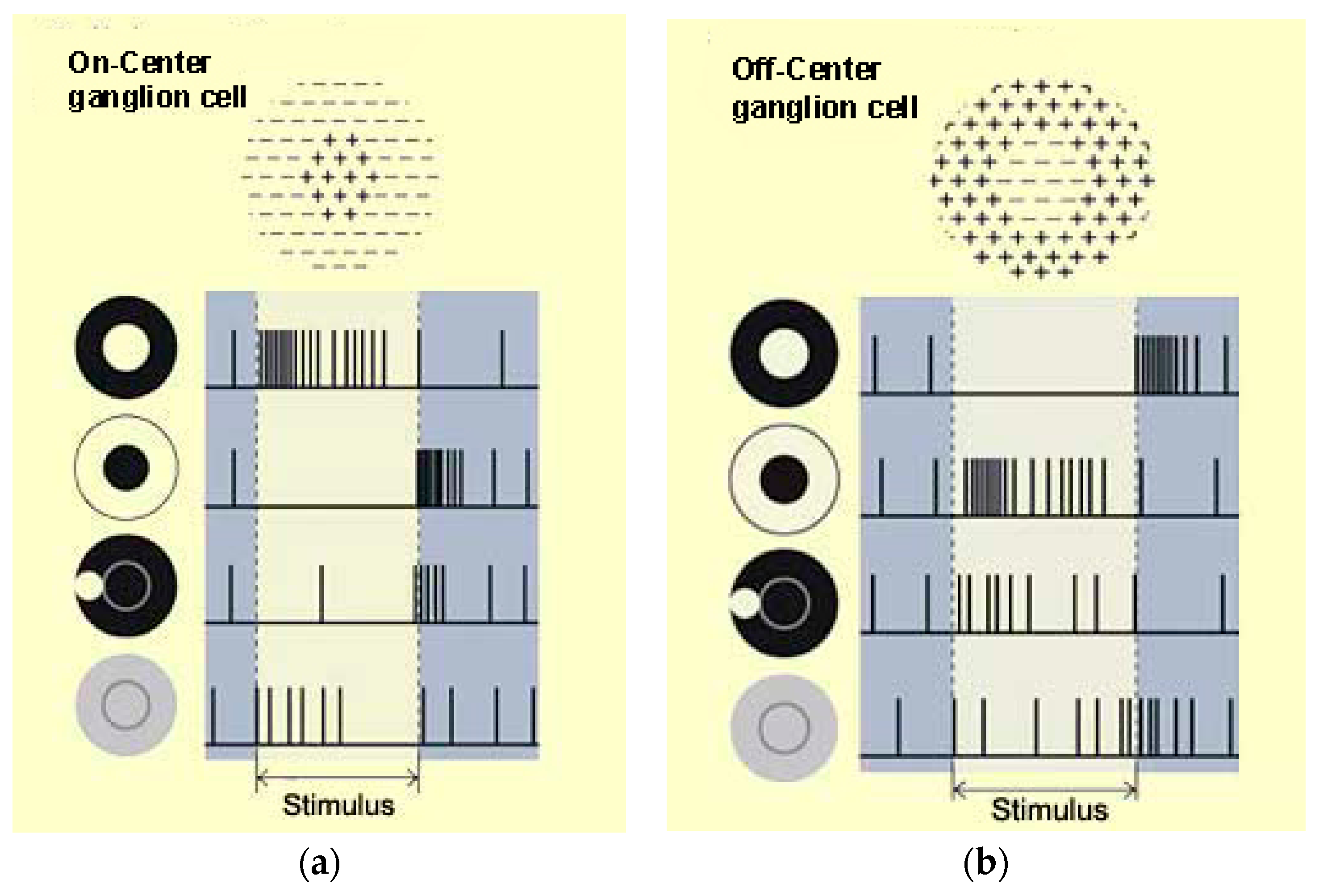
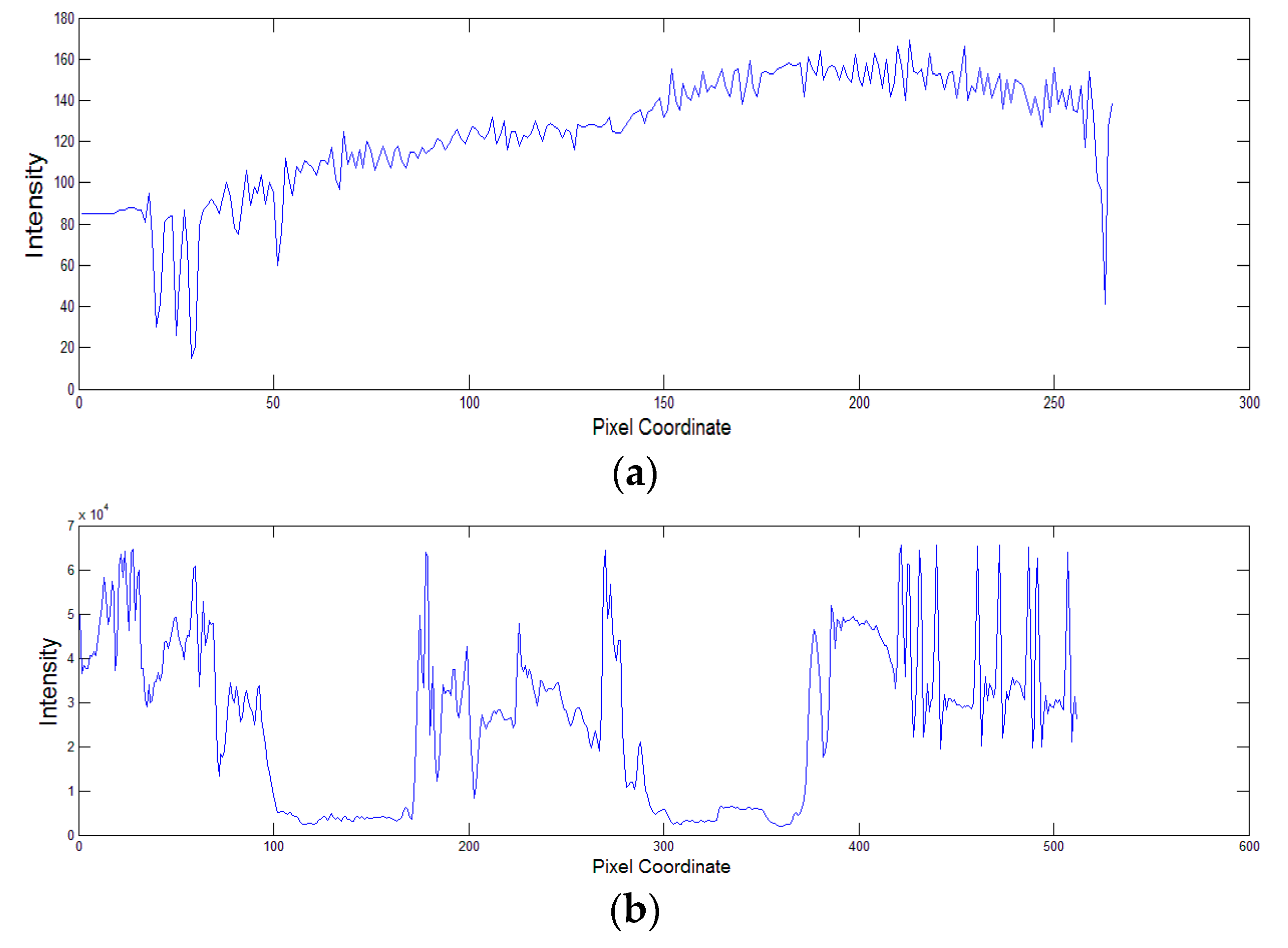
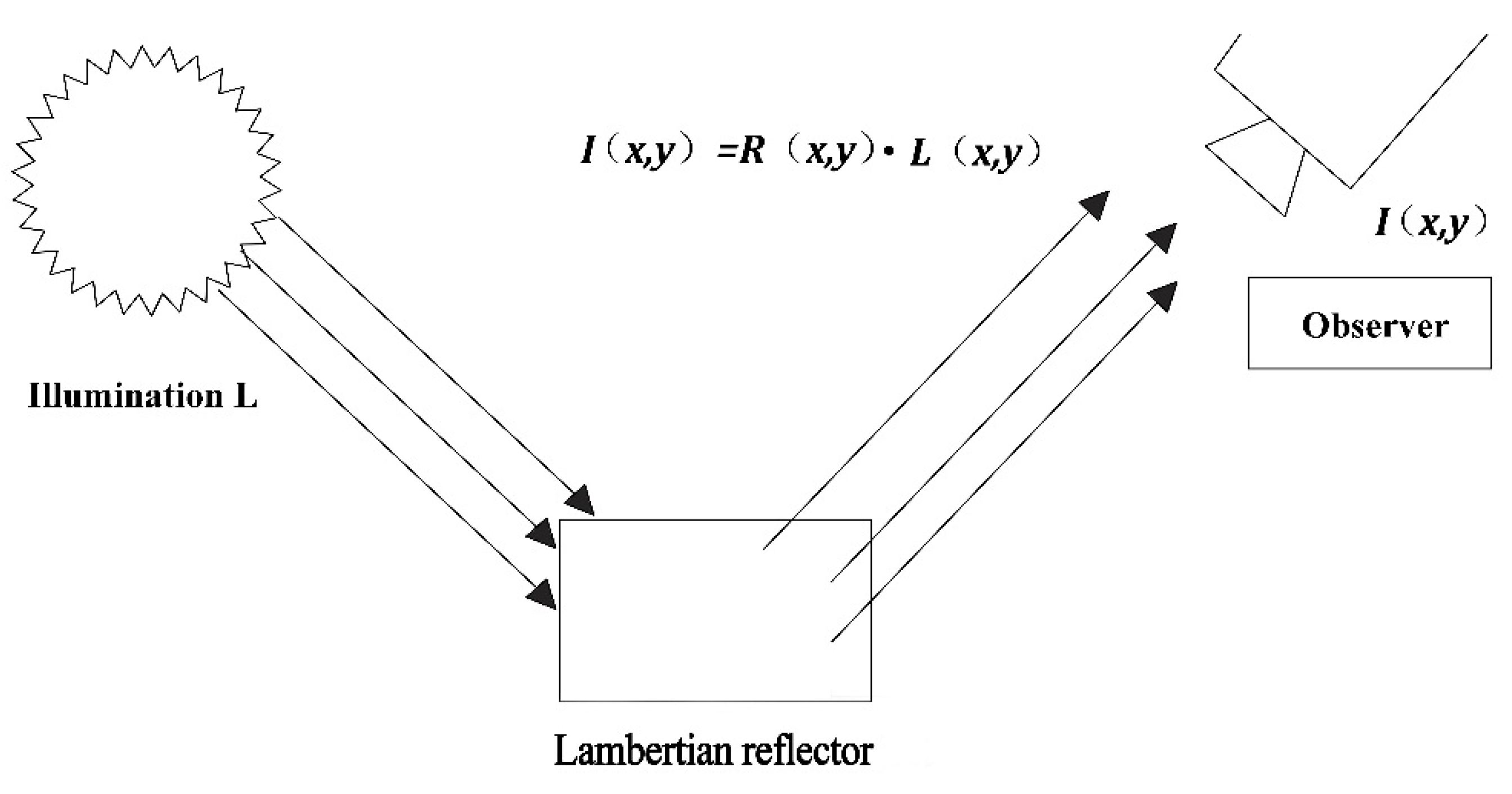
:1. Introduction
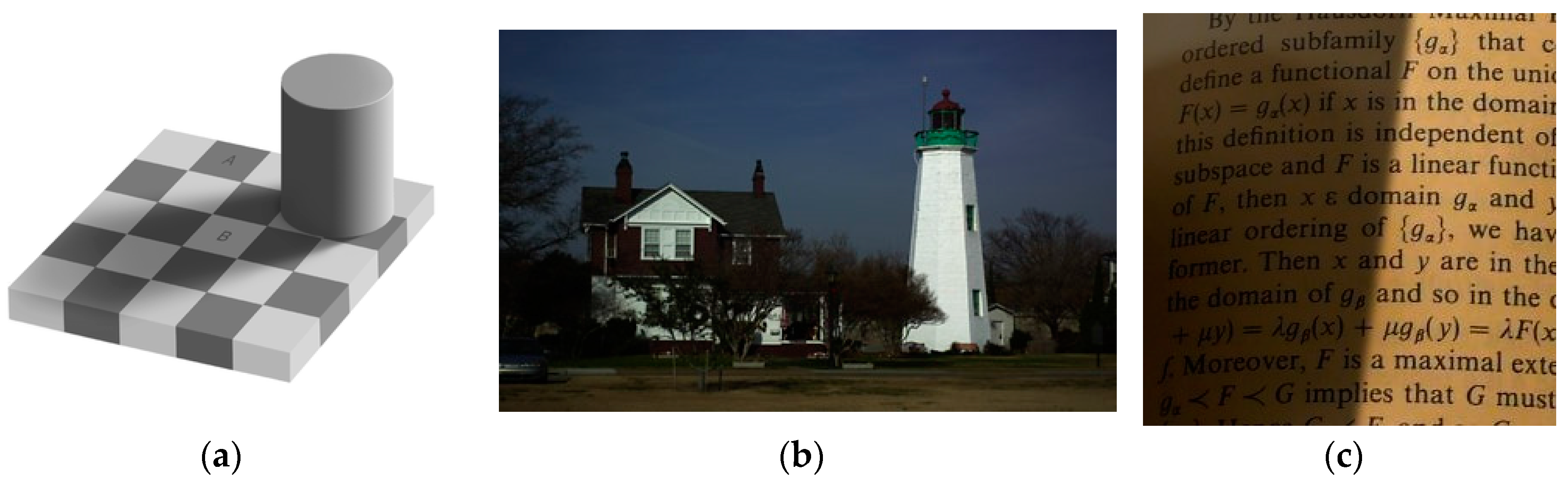
- (a)
- The reflecting object a Lambertian reflector and reflectance corresponds to sharp details in the image;
- (b)
- Illumination is smooth in most regions, but may contain non-smooth part(s).
2. New Assumption and Proposed Model
2.1. New Assumption
2.2. Proposed Model
2.3. Solution Existence
2.4. Implementation
2.4.1. Subproblem l with Fixed b and t
2.4.2. Subproblem b with Fixed l and t
| Algorithm 1: (Newton’s method) |
| Input: If Output Else while not converged End Output If Output Else End End |
- The illumination image, , becomes increasingly smooth over time.
- Diffusion speed in the tangent direction is always faster than that in the normal direction.
2.4.3. Update:
2.4.4. Update :
| Algorithm 2: (Variable Exponent Functional Retinex) |
| Input: Image Transform into log domain ; Initialization: , , and While (1) Given and , update by solving Equation (8). (2)Given and , update by using algorithm 1. (3)Update . (4) ; (5); End Output: Image |
2.5. Relation to Previous Methods
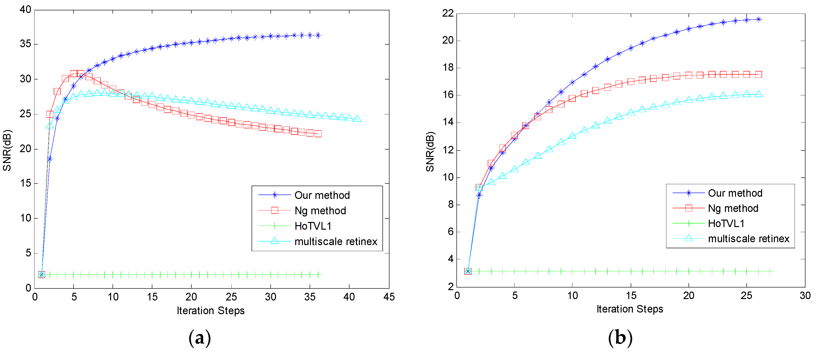
3. Numerical Results
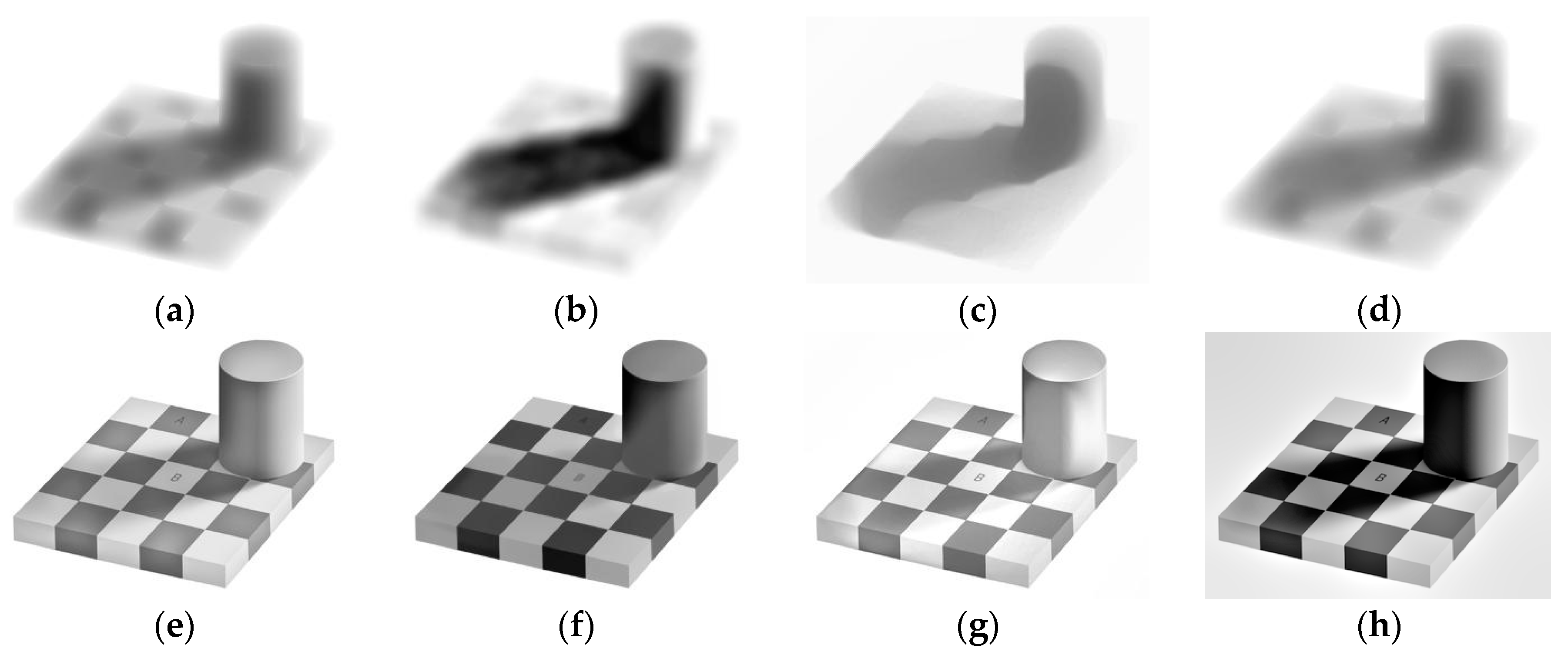
3.1. Synthetic Images
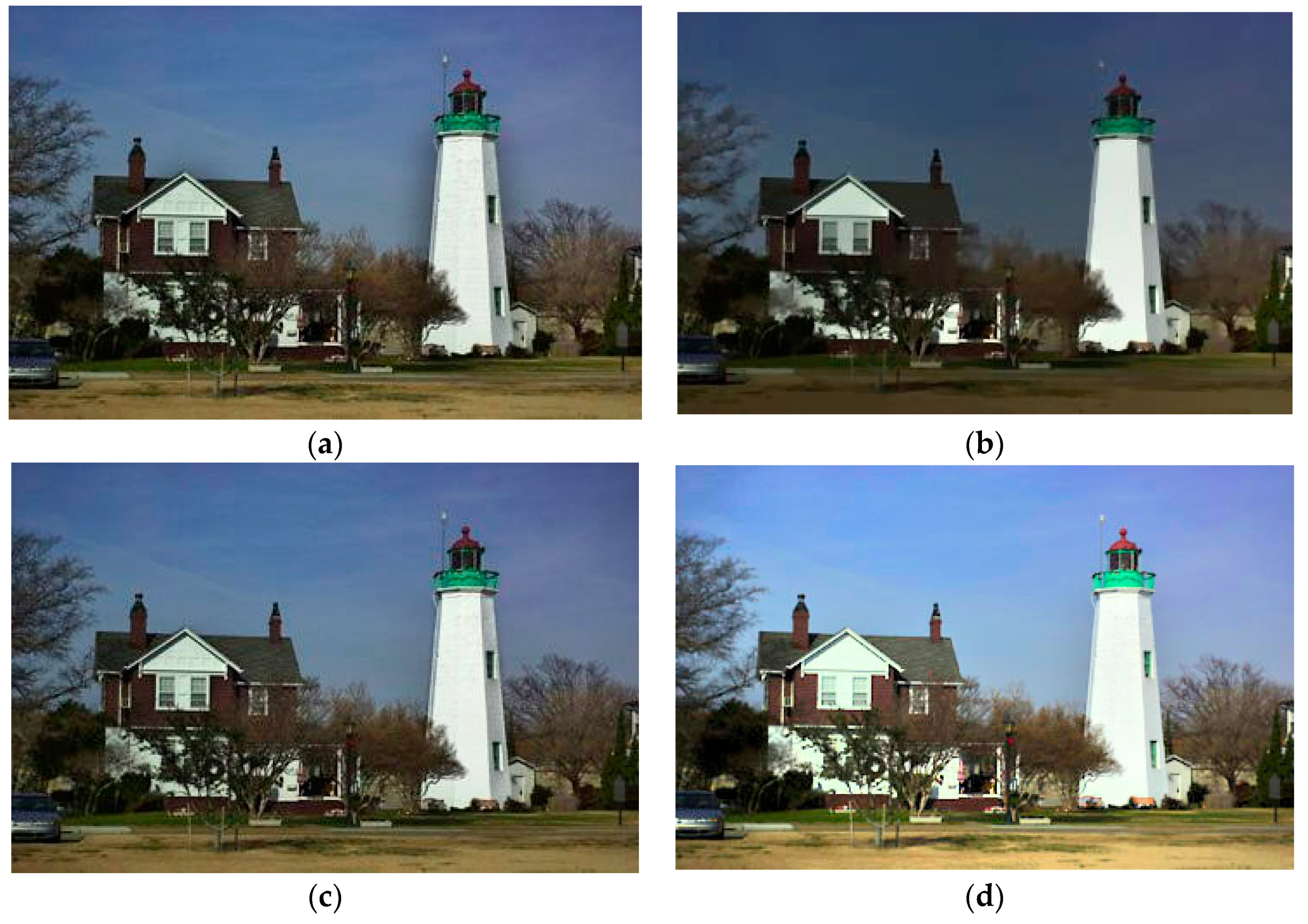
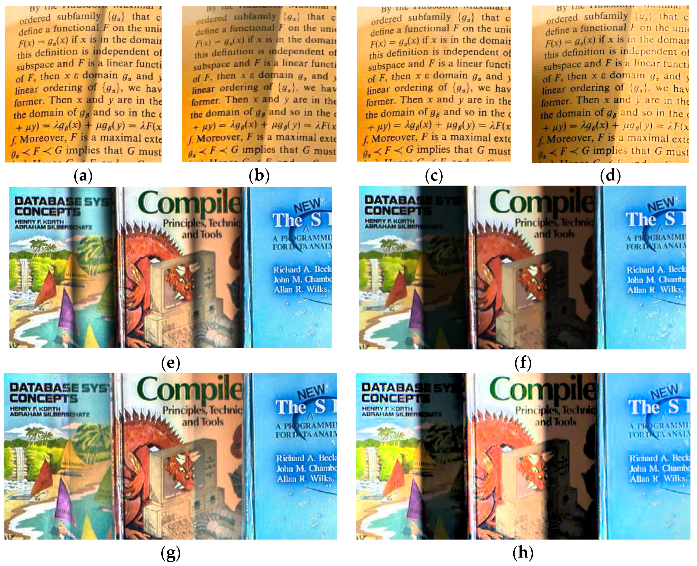
3.2. Natural Images
4. Conclusions
Acknowledgments
Author Contributions
Conflicts of Interest
References
- Visual System. Available online: https://en.wikipedia.org/wiki/Visual_system (accessed on 15 February 2016).
- Daw, N.; Goldfish, W. Retina: Organization for simultaneous color contrast. Science 1967, 158, 942–944. [Google Scholar] [CrossRef] [PubMed]
- Land, E.H. An alternative technique for the computation of the designator in the retinex theory of color vision. Proc. Natl. Acad. Sci. USA 1986, 83, 3078–3080. [Google Scholar] [CrossRef] [PubMed]
- Land, E.H.; McCann, J. Lightness and retinex theory. J. Opt. Soc. Am. 1971, 61, 1–11. [Google Scholar] [CrossRef] [PubMed]
- Alonso, J.M.; Chen, Y. Receptive field. Scholarpedia 2009, 4, 5393. [Google Scholar] [CrossRef]
- Lindeberg, T. A computational theory of visual receptive fields. Biol. Cybern. 2013, 107, 589–635. [Google Scholar] [CrossRef] [PubMed]
- Marini, D.; Rizzi, A. A computational approach to color adaptation effects. Image Vis. Comput. 2000, 18, 1005–1014. [Google Scholar] [CrossRef]
- Provenzi, E.; Marini, D.; de Carli, L.; Rizzi, A. Mathematical definition and analysis of the Retinex algorithm. JOSA A 2005, 22, 2613–2621. [Google Scholar] [CrossRef] [PubMed]
- Cooper, T.J.; Baqai, F.A. Analysis and extensions of the Frankle-McCann Retinex algorithm. J. Electron. Imaging 2004, 13, 85–92. [Google Scholar] [CrossRef]
- Funt, B.; Ciurea, F.; McCann, J. Retinex in MATLAB. J. Electron. Imaging 2004, 13, 48–57. [Google Scholar] [CrossRef]
- McCann, J. Lessons learned from mondrians applied to real images and color gamuts. In Proceedings of the Color and Imaging Conference, Scottsdale, AZ, USA, 16–19 November 1999; pp. 1–8.
- McCann, J.; Sobel, I. Experiments with Retinex; Technical Report for HPL Color Summit: Hewlett Packard Laboratories, Israel, 1998. [Google Scholar]
- Morel, J.M.; Petro, A.B.; Sbert, C. A PDE formalization of retinex theory. IEEE Trans. Image Process. 2010, 19, 2825–2837. [Google Scholar] [CrossRef] [PubMed]
- Kimmel, R.; Elad, M.; Shaked, D. A variational framework for retinex. Int. J. Comput. Vis. 2003, 52, 7–23. [Google Scholar] [CrossRef]
- Ma, W.; Morel, J.M.; Osher, S. An L 1-based variational model for Retinex theory and its application to medical images. In Proceedings of the IEEE Conference on Computer Vision and Pattern Recognition, Colorado Springs, CO, USA, 21–23 June 2011; pp. 153–160.
- Ma, W.; Osher, S. A TV Bregman iterative model of Retinex theory. UCLA CAM Rep. 2010, 10–13. [Google Scholar] [CrossRef]
- Ng, M.K.; Wang, W. A total variation model for Retinex. SIAM J. Imaging Sci. 2011, 4, 345–365. [Google Scholar] [CrossRef]
- Liang, J.; Zhang, X. Retinex by Higher Order Total Variation L1Decomposition. J. Math. Imaging Vis. 2015, 52, 345–355. [Google Scholar] [CrossRef]
- Zosso, D.; Tran, G.; Osher, S. Non-Local Retinex-A Unifying Framework and Beyond. J. SIAM Imaging Sci. 2015, 8, 787–826. [Google Scholar] [CrossRef]
- Dominique, Z.; Tran, G.; Osher, S. A unifying retinex model based on non-local differential operators. In Proceedings of the SPIE—The International Society for Optical Engineering, San Diego, CA, USA, 25–29 August 2013; pp. 1–12.
- Blomgren, P.; Chan, T.F.; Mulet, P. Total variation image restoration: numerical methods and extensions. In Proceedings of the IEEE Conference on Image Processing, Santa Barbara, CA, USA, 26–29 October 1997; pp. 384–389.
- Rudin, L.I.; Osher, S.; Fatemi, E. Nonlinear total variation based noise removal algorithms. Phys. D 1992, 60, 259–268. [Google Scholar] [CrossRef]
- Chen, Y.; Levine, S.; Rao, M. Variable exponent, linear growth functionals in image restoration. SIAM J. Appl. Math. 2006, 66, 1383–1406. [Google Scholar] [CrossRef]
- Li, F.; Li, Z.; Pi, L. Variable exponent functionals in image restoration. Appl. Math. Comput. 2010, 216, 870–882. [Google Scholar] [CrossRef]
- Xie, S.J.; Lu, Y.; Yoon, S. Intensity Variation Normalization for Finger Vein Recognition Using Guided Filter Based Singe Scale Retinex. Sensors 2015, 15, 17089–17105. [Google Scholar] [CrossRef] [PubMed]
- Meylan, L.; Süsstrunk, S. High dynamic range image rendering with a retinex-based adaptive filter. IEEE Trans. Image Process. 2006, 15, 2820–2830. [Google Scholar] [CrossRef] [PubMed]
- Diening, L.; Harjulehto, P.; Hästö, P. Lebesgue and Sobolev Spaces with Variable Exponents; Springer: Berlin, Germany, 2011. [Google Scholar]
- Goldstein, T.; Osher, S. The split Bregman method for L1-regularized problems. SIAM J. Imaging Sci. 2009, 2, 323–343. [Google Scholar] [CrossRef]
- Cai, J.F.; Osher, S.; Shen, Z. Split Bregman methods and frame based image restoration. Multiscale Model. Simul. 2009, 8, 337–369. [Google Scholar] [CrossRef]
- Nien, H.; Fessler, J.A. A convergence proof of the split Bregman method for regularized least-squares problems. SIAM J. Imaging Sci. 2014, 4371, 1402. [Google Scholar]
- Elvetun, O.L.; Nielsen, B.F. The split Bregman algorithm applied to PDE-constrained optimization problems with total variation regularization. Comput. Optim. Appl. 2016, 1–26. [Google Scholar] [CrossRef]
- Zou, J.; Fu, Y. Split Bregman algorithms for sparse group Lasso with application to MRI reconstruction. Multidimens. Syst. Signal. Process. 2015, 26, 787–802. [Google Scholar] [CrossRef]
- Chen, S.; Liu, H.; Hu, Z. Simultaneous Reconstruction and Segmentation of Dynamic PET via Low-Rank and Sparse Matrix Decomposition. IEEE Trans. Biomed. Eng. 2015, 62, 1784–1795. [Google Scholar] [CrossRef] [PubMed]
- Esser, E. Applications of Lagrangian-based alternating direction methods and connections to split Bregman. CAM Rep. 2009, 9, 31. [Google Scholar]
- Stephen, B.; Neal, P.; Eric, C. Distributed optimization and statistical learning via the alternating direction method of multipliers. Found. Trends Mach. Learn. 2011, 3, 1–122. [Google Scholar]
- Petro, A.B.; Sbert, C.; Morel, J.M. Multiscale retinex. IPO 2014, 71–88. [Google Scholar] [CrossRef]
- Buttkus, B. Homomorphic filtering—Theory and practice. Geophys. Prospect. 1975, 23, 712–748. [Google Scholar] [CrossRef]


| Image | Ng | HoTVL1 | Proposed Method | Multiscale Retinex |
|---|---|---|---|---|
| Figure 7a | 0.9076 | 0.6342 | 0.9289 | 0.8764 |
| Figure 7d | 0.7603 | 0.6633 | 0.8291 | 0.7238 |
| Image | Ng | HoTVL1 | Proposed Method | Multiscale Retinex |
|---|---|---|---|---|
| Figure 7a | 26.8927 | 29.6729 | 26.6182 | 27.9038 |
| Figure 7d | 24.5474 | 26.0115 | 21.9972 | 25.4528 |
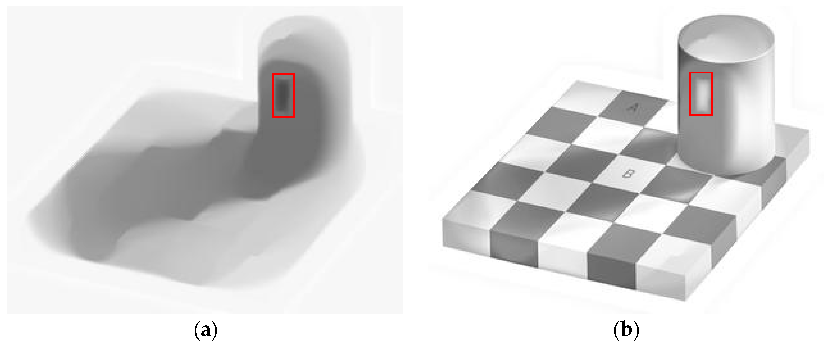
| Image | Original | Ng | HoTVL1 | Proposed Method | Multiscale Retinex | |
|---|---|---|---|---|---|---|
| Checkerboard | A | 120 | 140 | 85 | 135 | 109 |
| B | 120 | 180 | 174 | 230 | 149 |
© 2016 by the authors; licensee MDPI, Basel, Switzerland. This article is an open access article distributed under the terms and conditions of the Creative Commons Attribution (CC-BY) license (http://creativecommons.org/licenses/by/4.0/).
Share and Cite
Dou, Z.; Gao, K.; Zhang, B.; Yu, X.; Han, L.; Zhu, Z. Realistic Image Rendition Using a Variable Exponent Functional Model for Retinex. Sensors 2016, 16, 832. https://doi.org/10.3390/s16060832
Dou Z, Gao K, Zhang B, Yu X, Han L, Zhu Z. Realistic Image Rendition Using a Variable Exponent Functional Model for Retinex. Sensors. 2016; 16(6):832. https://doi.org/10.3390/s16060832
Chicago/Turabian StyleDou, Zeyang, Kun Gao, Bin Zhang, Xinyan Yu, Lu Han, and Zhenyu Zhu. 2016. "Realistic Image Rendition Using a Variable Exponent Functional Model for Retinex" Sensors 16, no. 6: 832. https://doi.org/10.3390/s16060832
APA StyleDou, Z., Gao, K., Zhang, B., Yu, X., Han, L., & Zhu, Z. (2016). Realistic Image Rendition Using a Variable Exponent Functional Model for Retinex. Sensors, 16(6), 832. https://doi.org/10.3390/s16060832