Abstract
The purpose of this article is to describe the design of a limited stroke actuator and the corresponding prototype to drive a Low Pressure (LP) Exhaust Gas Recirculation (EGR) valve for use in Internal Combustion Engines (ICEs). The direct drive actuator topology is an axial flux machine with two air gaps in order to minimize the rotor inertia and a bipolar surface-mounted permanent magnet in order to respect an 80° angular stroke. Firstly, the actuator will be described and optimized under constraints of a 150 ms time response, a 0.363 N·m minimal torque on an angular range from 0° to 80° and prototyping constraints. Secondly, the finite element method (FEM) using the FLUX-3D® software (CEDRAT, Meylan, France) will be used to check the actuator performances with consideration of the nonlinear effect of the iron material. Thirdly, a prototype will be made and characterized to compare its measurement results with the analytical model and the FEM model results. With these electromechanical behavior measurements, a numerical model is created with Simulink® in order to simulate an EGR system with this direct drive actuator under all operating conditions. Last but not least, the energy consumption of this machine will be estimated to evaluate the efficiency of the proposed EGR electromechanical system.
1. Introduction
1.1. Automotive Context
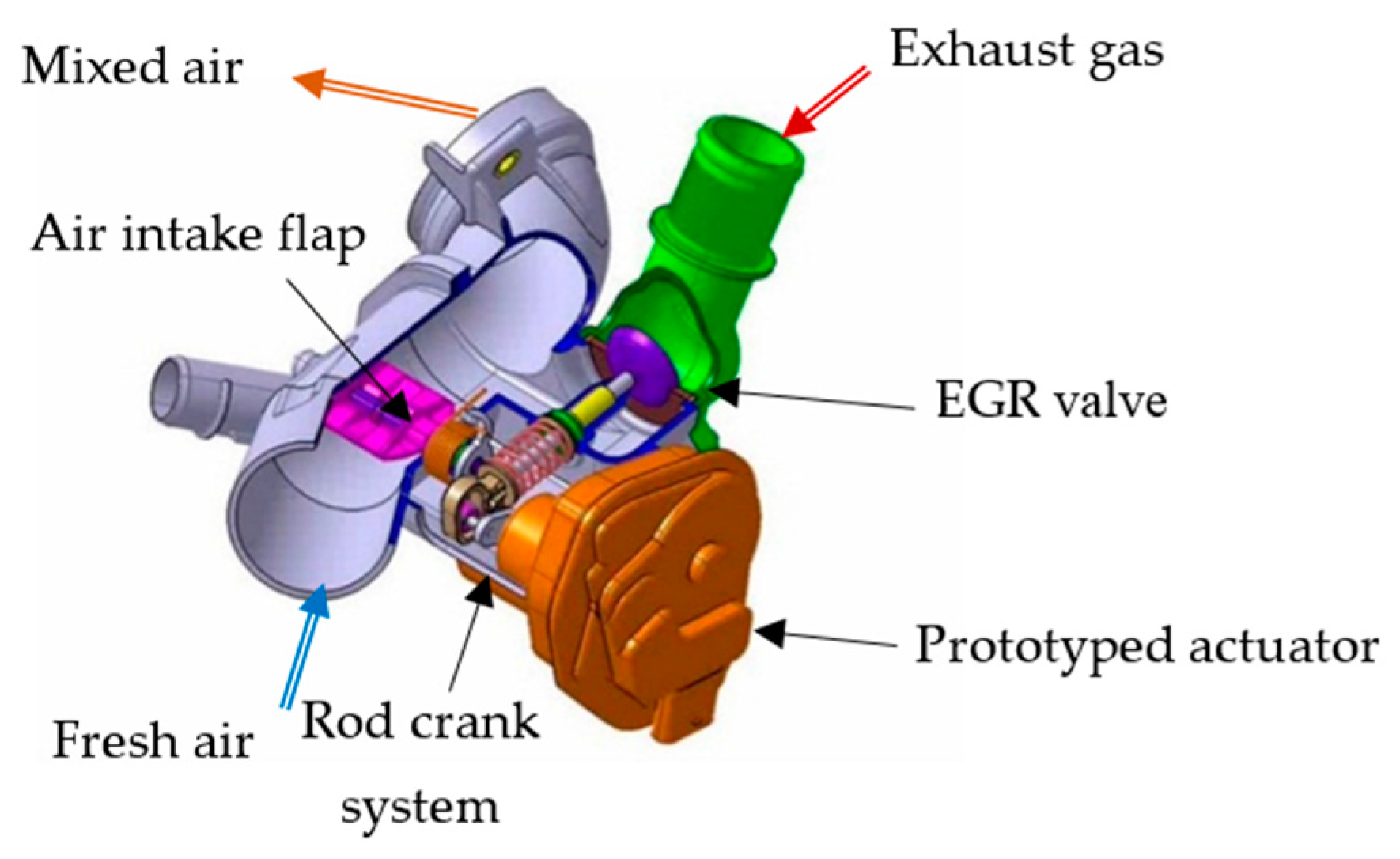
In order to reduce greenhouse gases and the polluting emissions of new vehicles, new internal combustion engine concepts need a new regulation management of air flow as described in [1,2]. As shown in [1] and Figure 1, Mann and Hummel proposed a dual air loop EGR system using an EGR Low Pressure (LP) valve and air flow throttle. This system is more adapted to plastic use as opposed to the topology using an exhaust throttle as presented in [2]. The use of an intake valve also leads to lesser stress on the DC motor and electronic components.

Figure 1.
Air flow and EGR system of an internal combustion engine with the actuator prototype.
As we can see from the drawing in Figure 1, the actuator moves this mechanism in two steps through a rod-crank system. In the first step, the actuator moves the EGR valve and opens the EGR circuit loop in order to mix exhaust gas with fresh air. Then, when the EGR valve is wide open, as it can be necessary to improve the EGR rate, the actuator closes the fresh air circuit with the air intake flap.
To drive this EGR mechanical system, a state of the art electromechanical actuator, that manages the air flow, as described in [3,4,5], has been identified and several electrical DC machine structures analyzed. There are two main electric topologies which produce rotary movements: the first one is an indirect drive [5], composed of a brushed DC machine as in [6] and a reduction gear set, the second one is a direct drive machine such as a torque motor defined by a single phase BLDC machine. The two topologies are prototyped and presented in Figure 2.
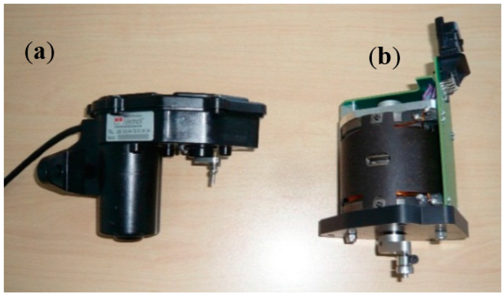
Figure 2.
Indirect and direct drive actuator prototypes: (a), the indirect drive actuator, (b) the direct drive actuator. As presented in [7], both actuators are optimized with the same requirements in order to compare their energy consumptions.
For the application and this paper, the direct drive actuator has been chosen for its reliability as well as its time response qualities in order to avoid the non-linear behaviour of the gear set of an indirect drive actuator. The 80° angular stroke requirement implies that the actuator is defined by a bipolar permanent magnet in order to produce a constant and high torque for a given value of current on a 180° theoretical stroke (more or less 120° in reality). This actuator is designed in two steps.
1.2. Choice of Actuator Topology
First, in order to choose an electrical machine concept, references [8,9,10] describe some Limited Angle Torque Motor (LATM) topologies with a toroidally wound armature. This topology has its pros and cons. In many ways, from the torque per unit volume and manufacture point of view, the concentrated winding is preferred to respect some requirements constraints. A comparative study of five magnetic structures is described in [11] with two radial flux machines with an internal or external rotor and three axial flux machines topologies with one or two air gaps. Each topology is composed of concentrated windings and a ferromagnetic core on the stator, and then a surface mounted permanent magnet on the rotor. A ferromagnetic part on the rotor might be used in some cases. The comparative study shows a simple analytical model in which the sizing parameters of the actuator geometry and the electromagnetic characteristics are defined. Then an optimization objective is used to calculate the optimal values of these parameters in order to minimize the actuator volume according to the physical and merely dynamic constraints.
In this case, the magnetic concept results show that radial flux machines are better than axial flux machines for their performance in restricted volumes. Nevertheless, axial flux machines are more interesting for their flat form magnets and the concentrated windings that are simpler to produce. The final result of this comparative study on actuating concepts shows that an axial flux machine with two air gaps with a central rotor without ferromagnetic part is more attractive for its flat form magnet and its low rotor inertia.
1.3. Axial Flux Machine Design Approach
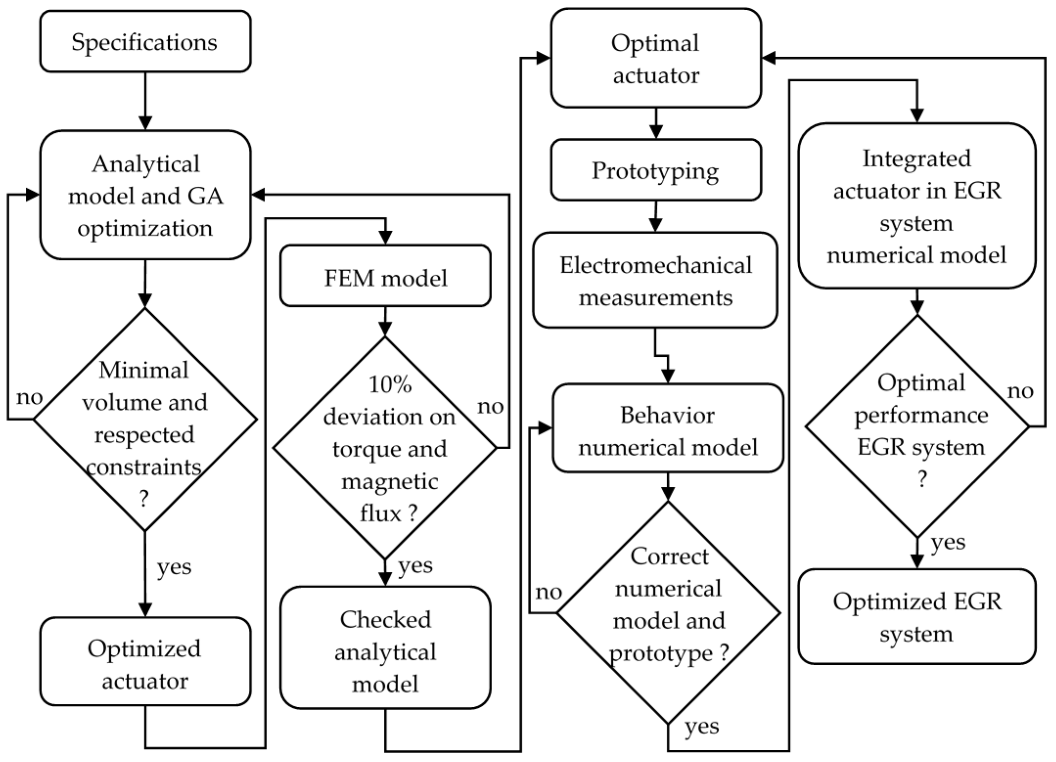
In a second part, an optimization to minimize the actuator volume and to consider the others constraints such as the prototyping and manufacturer constraints is demonstrated. The results are checked with the FEM with FLUX-3D in non-linear mode. Then the prototype and its characterization can be realized in order to simulate the EGR mechanical behavior under all conditions. The design flowchart to define the optimal actuator to drive an EGR mechanical system is summarized in Figure 3.
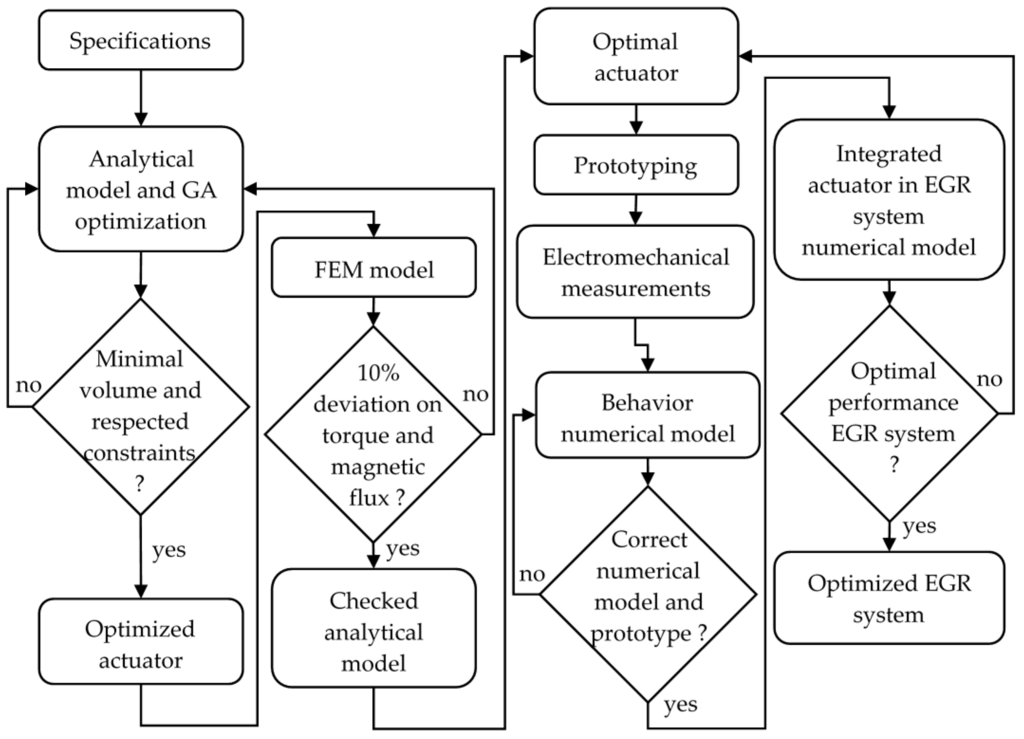
Figure 3.
The flowchart procedure to design the prototype direct drive actuator.
2. Analytical Model
To write the flux and torque expressions, the air gap magnetic flux density must be defined. A cylindrical reference (r,α) is fixed to the stator in order to visualize the magnetic flux density. A moving cylindrical reference (r,θ) is fixed to the rotor to visualize the actuator torque. θ is a rotational angle of the rotor with respect to α = 0°. Figure 4 presents the rotor and stator cylindrical references.
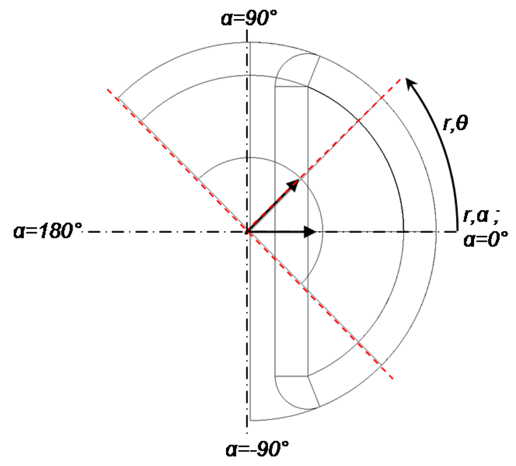
Figure 4.
Rotor and stator cylindrical references.
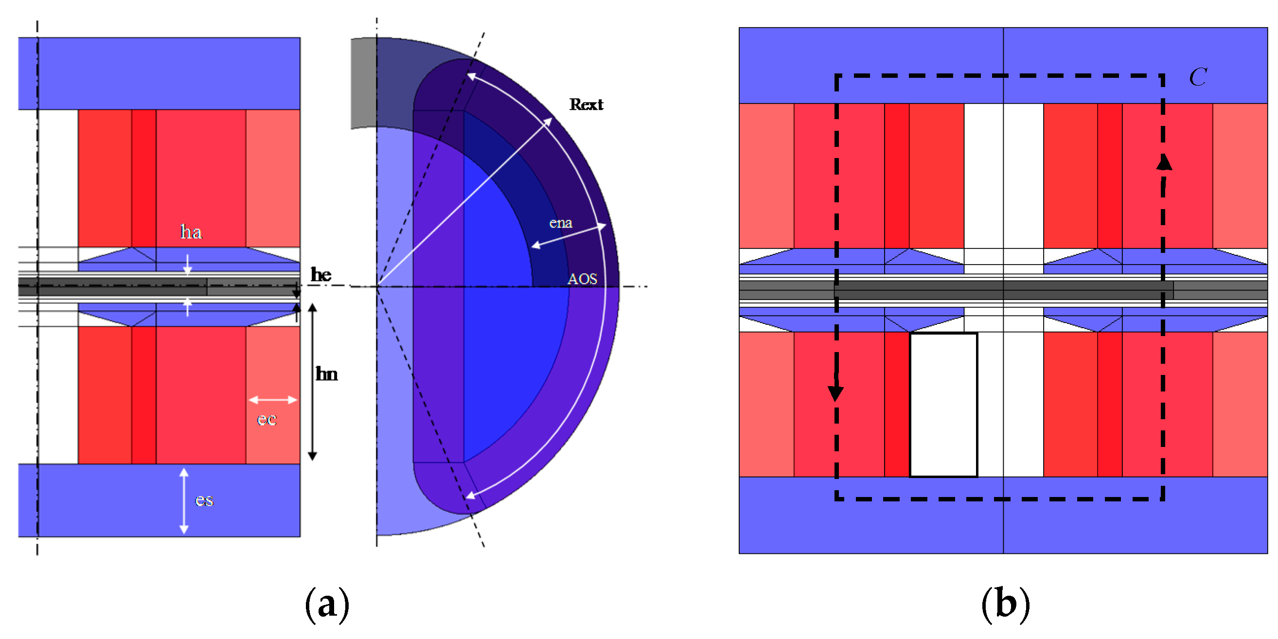
The actuator is a bipolar permanent magnet composed of four coiled concentrated windings and two magnets in the rotor. Figure 5 shows the axial flux actuator topology.

Figure 5.
Direct drive actuator parameters (a) and the flux line contour C in axial flux machine (b).
2.1. Air Gap Magnetic Flux Density Calculation
As presented in [4], the analytical model calculates the actuator torque in accordance with the magnetic flux produced by magnets and the magnetomotive force fmm. The relation of the magnetomotive force depends on n, which is the number of turns in a slot pair and I, the current in each coil for knI coils. Ampere’s law on C path is applied for each actuator, flux crosses ke times an air gap thickness e and ka times magnet thickness ea:
where Ha is the magnet field and He the air gap field. Then, with the magnetic field in air gap law, magnet field law, and conservative flux law, the magnetic flux density in the air gap Be can be defined by the sum of the magnets’ flux density part and the fmm part such as:
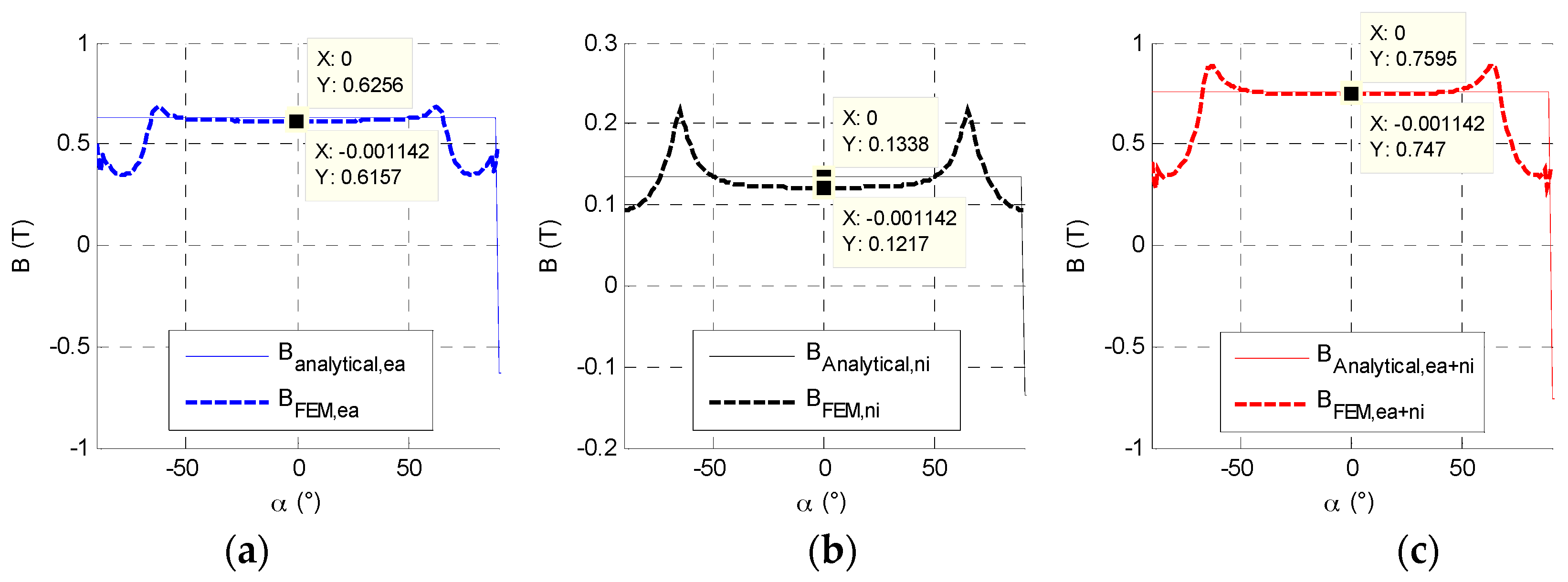
where µ0 is the vacuum permeability, µr the magnet relative permeability and Br the remanent flux density of magnet and Ba the magnetic flux density in magnet. Functions β and δ equal −1 or 1 according to the observation position in the air gap as shown in Figure 6. The magnets’ flux density, Bea, depends on the rotor position according to θ. The stator current reaction, Bni, is fixed whatever the rotor position. The resulting flux density in the air gap, Be, is the sum of both.
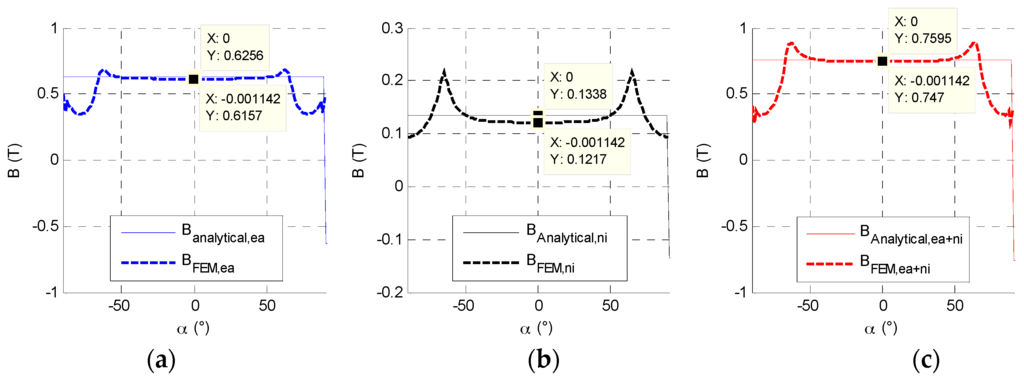
Figure 6.
The distributed induction flux density in the air gap: (a) magnet induction flux density Bea; (b) the magnetomotrice force flux density Bni; (c) sum of both Be on a complete pole pitch.
2.2. Excitation Flux Expression and Saturation Constraints
The magnet flux depends on θ the rotor position with regard to stator. The excitation flux in air gap is defined by:
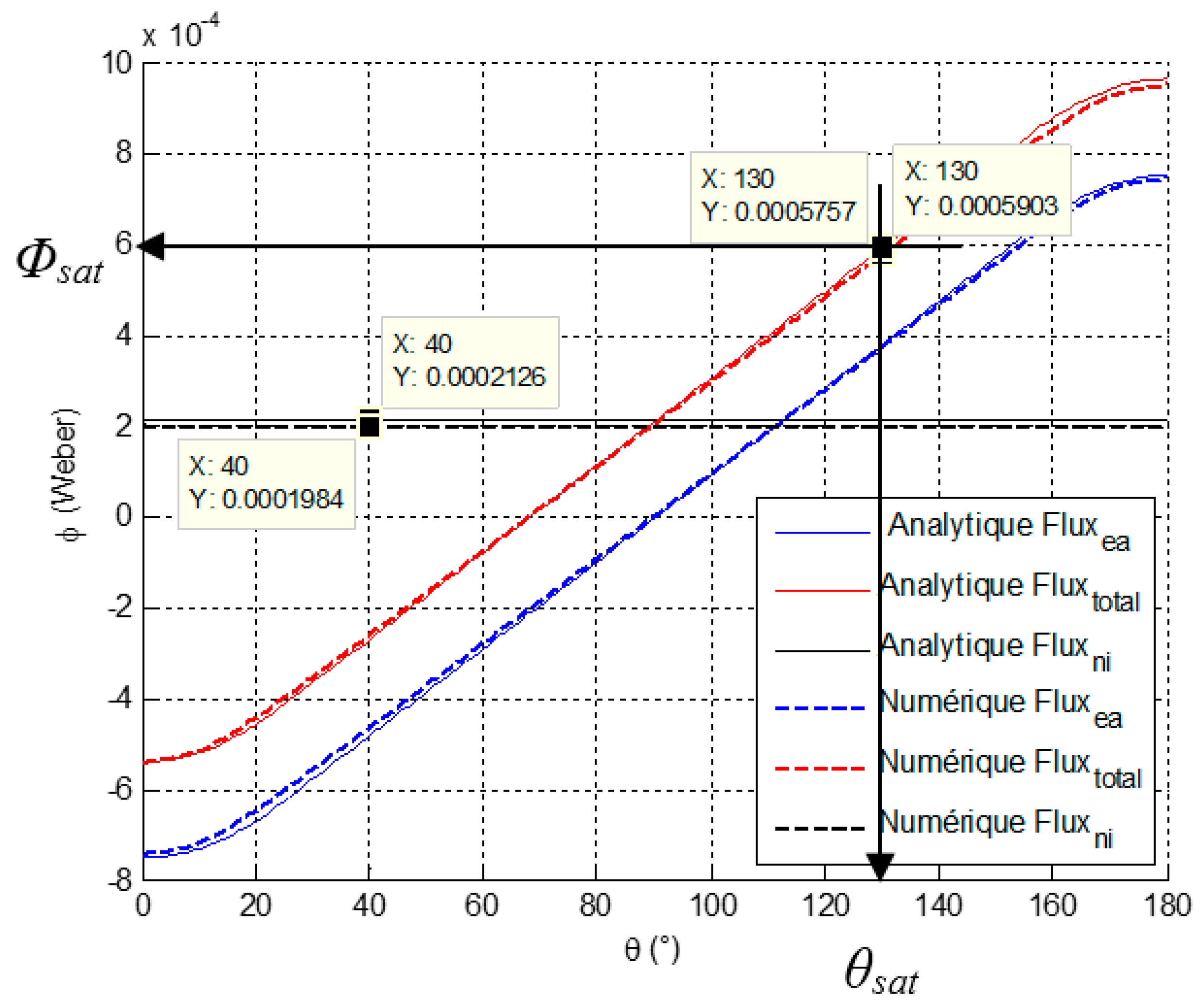
The magnets flux Φea, depends on the rotor position, the curve is variable according to θ. The stator current reaction, Φni, (with Φleakage integrated) is fixed whatever the rotor position. The resulting flux Φe is the sum of both. Figure 7 presents each magnetic flux part.
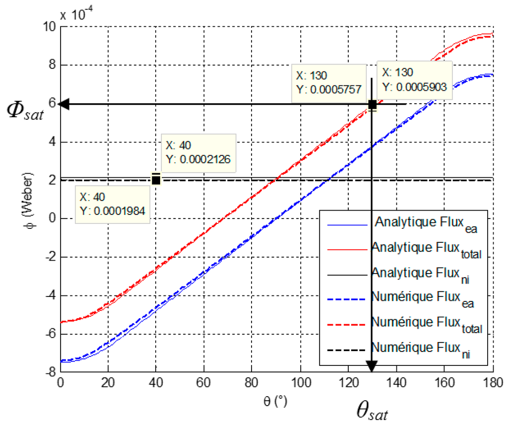
Figure 7.
Magnetic flux evolution observed by a coiled polar tooth.
The magnetic flux is used to define the actuator geometry according to the saturation induction level. The maximum magnetic flux densities in the rotor and stator are calculated with the Φsat maximal flux that crosses the rotor and stator section at the last rotor position θsat according to the end of stroke. For example at the θsat rotor position equal to 130°, the magnetic circuit is designed with the Φsat magnetic flux value at this point. Saturation flux density is calculated in the magnetic circuit such as:
2.3. Torque Definition
The torque value is defined by the variation of the magnetic flux. In magnetic coenergy derivative, the part of the flux varies according to the rotor position θ from between 0° and 180° such as:
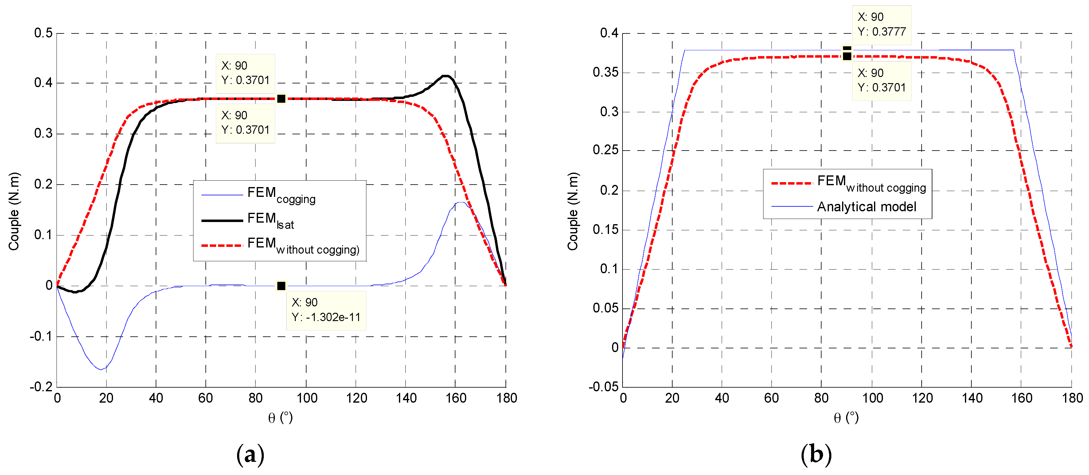
The cogging torque is not modelled in the analytical model. The FEM resolution is linear and the obtained torque includes the cogging effect. In order to compare analytical and FEM torques, the cogging torque values are subtracted from the torque FEM result at saturation current. Figure 8 presents the torque evolution according to the rotor position and the influence of a polar tooth’s opening angle.
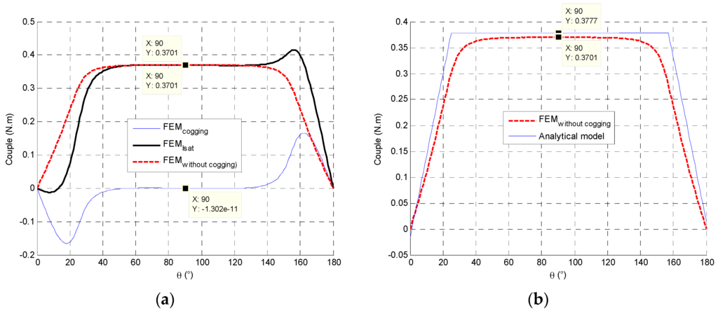
Figure 8.
(a) The FEM torque evolution between cogging torque and torque at fixed current; (b) The torque comparison in a linear behavior between the analytical model and FEM model.
Then, the linear constant torque between torque computation and the current in the coil can be obtained:
2.4. Magnets Thickness Constraints
Permanent magnets are made of rare earth alloys because of their high energy characteristics. The magnet model is simplified for the analytical study. From Equation (2), the magnet minimal thickness should verify the following condition to avoid demagnetization:
2.5. Electrical Resistance and Inductance Coils
The geometrical definition implies an l wire length. Its length depends of quantity of coil turns n that it is possible to place in the slot section in accordance with the enameled copper wire section Scu. The electrical resistance of the actuator, composed of four coils, is written as:
The electrical resistivity at 130 °C is 24.3 × 10⁻⁸ Ω·m. The inductance coils expression is written in accordance with the magnetic flux Φ and the current I:
2.6. Total Inertia at the Actuator Shaft End
To move the EGR system with a 150 ms time response on 80° stroke, the actuator develops a torque according to the sum of all inertia. The total inertia of the system is composed by the magnet inertia and a drive shaft inertia such as Jm and then the EGR system inertia such as Jload such as:
Then, according to a uniform acceleration and deceleration, the actuator torque should be higher than the sum of inertia and load Tload such as:
2.7. Electromechanical Behavior
At this stage, the optimization doesn’t consider a closed loop control. Nevertheless, in order to respect the required response time like a closed loop control system as presented in [12], a position cycle is described with a 150 ms flap position response time including acceleration and deceleration for the forward and backward travel as shown in Figure 9. The optimization method has to calculate the switching time in compliance with the flap position specification on a forward and backward travel from 0° to 80°.
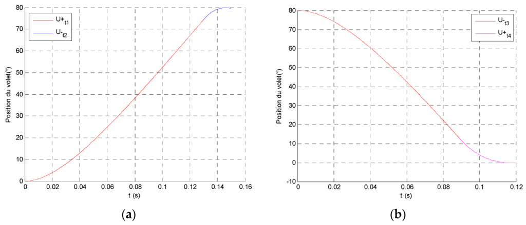
Figure 9.
The uniform accelerating and decelerating trajectories; (a) forward and (b) backward travels.
Electrical and mechanical balances are expressed as:
To calculate the rotor position versus supply voltage time, the electrical balance and mechanical equations must be solved. Inductance values cannot be ignored and this involves a state-space model to compute the acceleration, speed and then the position of actuator. The electromechanical balance is written by this state-space matrix:
3. Optimization and Results
The state of the art of the Genetic Algorithm (GA) is described in [13]. The GA is a one of the most popular algorithms to optimize electrical devices and it has been used to optimize the model parameters of the analytical model.
3.1. Algorithm Optimization
A numerical software such as MATLAB® is used for the optimization. The GA is coded in real time with it. The GA is a sequence of a selection, mutation and crossover of individuals from a population as described in [13]. An individual is a parameter vector composed by genes. A gene is a variable parameter of the actuator who takes an integer value between a minimal and a maximal limit. Elitism is used to conserve the best individuals of a generation. This strategy copies the best individual from generation n − 1 into generation n. GA converges to the global best individual who defines the optimized actuator. The optimization objective is to minimize the volume. The population is composed of 200 individuals. The crossover coefficient is equal to 70% and the mutation to 0.1%. 50% of best individuals, who respect the constraints, are conserved from generation n − 1 into generation n and the 50% part of the population are created according to the crossover and the mutation. If the minimal volume doesn’t vary anymore after 200 generations, GA stops the optimization. We then consider that the objective has been reached.
3.2. Functioning Conditions and Constraints
The axial flux machine is optimized in the worst operating case of the EGR system. The functioning condition are:
- a 130 °C temperature,
- a 9 V supply voltage,
- a 363 mN·m minimal torque at the end of stroke,
- a 150 ms time response for a 80° angular stroke.
In order to define the number of coils turns, a continuous evolution of enameled copper wire diameter is defined between 0.1 and 2.5 mm. Besides, the magnet material is defined with a 1 T magnet remanent flux density Br at 130 °C with a relative permeability µa equal at 1.03. A 0.8 mm air gap thickness e is chosen. The constraints are the following:
- the stator and rotor flux density should be lower than 1.57 T at the end of stroke, because of the saturation magnetic flux Φsat with a 4500 maximal relative permeability, as defined in [14],
- the magnet thickness (Equation (6)) should be higher than the demagnetization magnet thickness,
- the actuator torque should be higher than the sum inertial of torque and required torque on a 92° minimum stroke range (to include edge effect),
- the electromechanical time constant is three times lower than the response time,
- the current density is limited at 5 A/mm2 in the slot section,
- the maximal current is 10 A.
To respect dynamic needs and to avoid too restrictive a calculation, 5% tolerance on the output shaft position at the end of stroke is used during the calculation. This tolerance affects the forward and backward acceleration times and consequently, the optimization can accept a large of number of good candidates who respect electromechanical constraints.
3.3. Optimization Results
At the optimization start point, the analytical model computes a 238 cm3 actuator volume. After 3233 generations and a 67,326 s computation time, at the end of optimization, the optimal actuator volume is 198 cm3 with the respected constraints. Table 1 shows the optimized variable parameter values.

Table 1.
Optimized parameter values.
The optimized direct drive actuator is characterized with a 90 mN·m/A constant torque, a 1.12 ohm electrical resistance and a 23.7 mH electrical inductance at 25 °C, and then, a 0.8 × 10⁻⁵ kg·m2 rotor inertia.
3.4. FEM Checking in Linear and Saturated Behavior
The analytical model actuator is defined with a linear magnetic material model without B-H saturation curve. Table 2 shows the difference between the analytical and FEM linear results for a 5.72 A saturation current. The linear behavior, analytical results and FEM results are similar.
Table 2.
Linear magnetics results of optimized actuator.
Moreover, if the actuator is a good design, at the saturation current and for the 130° rotor position, the actuator core reaches a 1.57 flux density. At the moment, FLUX-3D can’t compute a B-H hysteresis loop of magnetic materials. A B-H saturation curve is defined by an Arctan function such as used in FLUX-3D, as defined in [15] and presented in Figure 10 below.
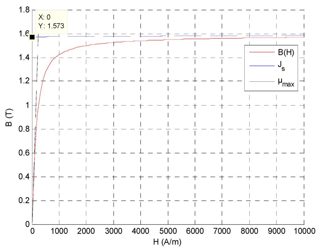
Figure 10.
The B-H saturation curve for a 1.57 T saturation induction and a 4500 relative permeability.
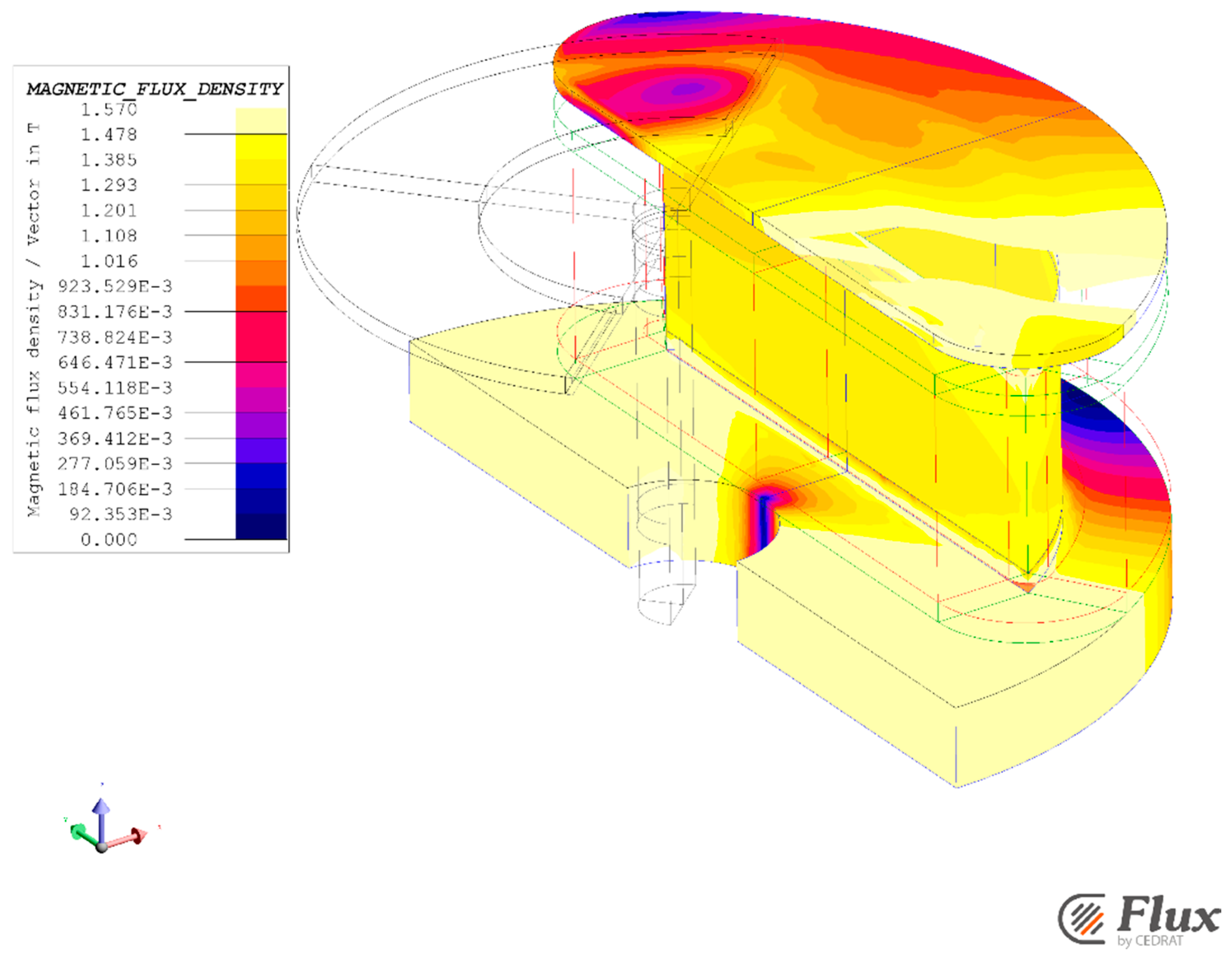
As shown in Figure 11, all in all, the stator flux density level shows at the 130° rotor position that the actuator geometry seems to respect the saturation constraints at less than 1.57 T in the core.

Figure 11.
Magnetic flux density in core at the 130° rotor position and the 5.72 A current.
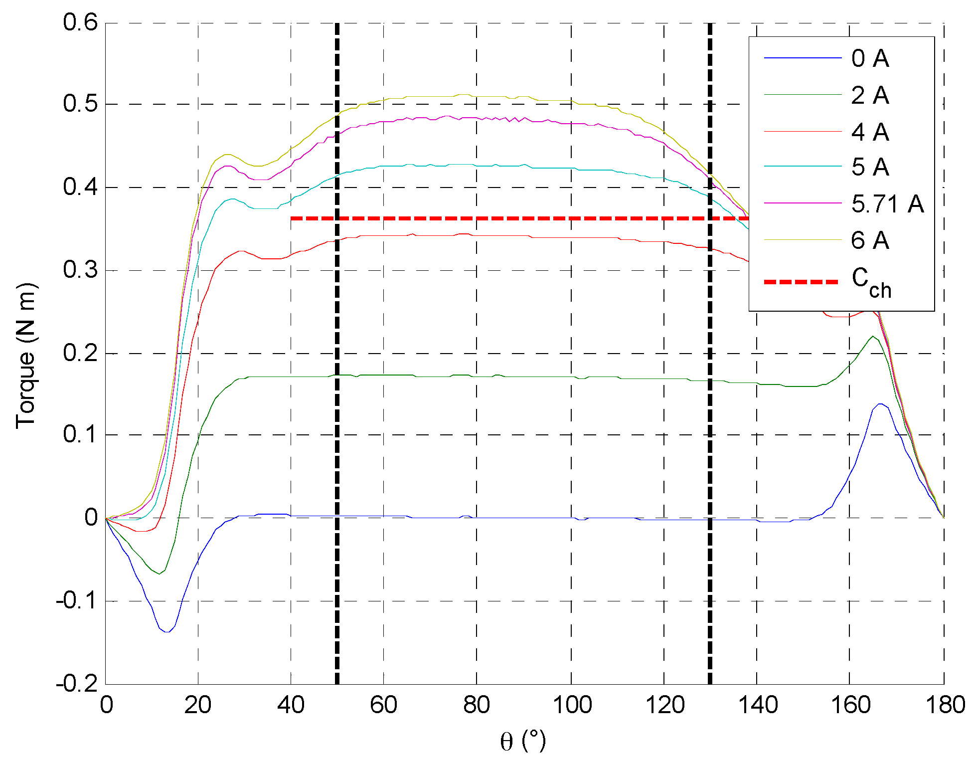
However, the analytical model is a mean model, so the located saturation can’t be estimated. In the linear behavior, the flux density in the first part of the teeth is higher than the 1.57 T and this point can be overlook since the 80° angular range of the actuator is between from 50° to the 130° rotor position such as presented in Figure 12.
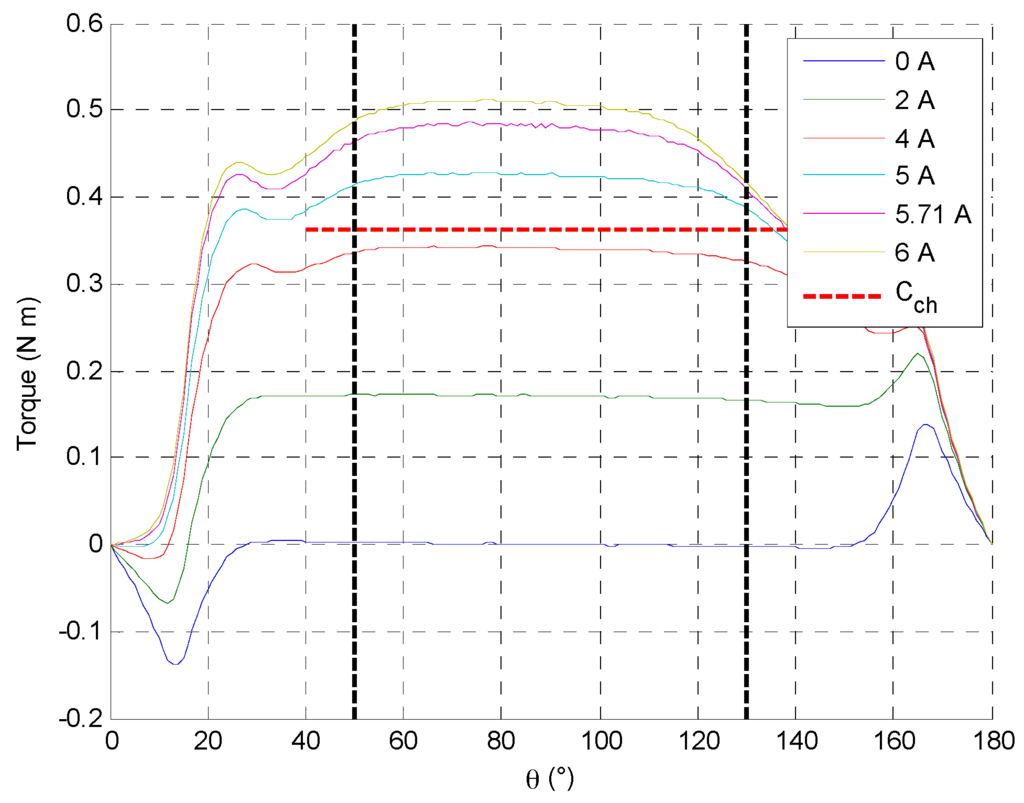
Figure 12.
Torque actuator evolution at different positive current and rotor position.
The comparison between analytical model and FEM model are correct as presented in Table 3. The prototype can be realized and characterized.
Table 3.
Performance comparison.
4. Actuators Characterization to Build an Electromechanical Behavior Model
To drive the prototyped actuator, a power electronics and a control are defined. The EGR system needs a reversibility control in forward and backward travel. The power electronics is defined by a H-bridge with a low ohmic resistance (0.2 Ohm including wiring). Then, in order to control the shaft position, a control system is defined with a Hall Effect position sensor, developed by EFI Automotive [16], integrated in output shaft end of the direct drive actuator and a microcontroller with the control law implemented.
4.1. Mechanical and Electric Behaviors Measurements
The electrical resistance and magnet remanent flux density display a linear behavior according to the temperature. However, the ferromagnetic characteristics of the core give some nonlinear effects on torque and inductance values in accordance with the core saturation flux density.
4.1.1. Non-Linear Torque
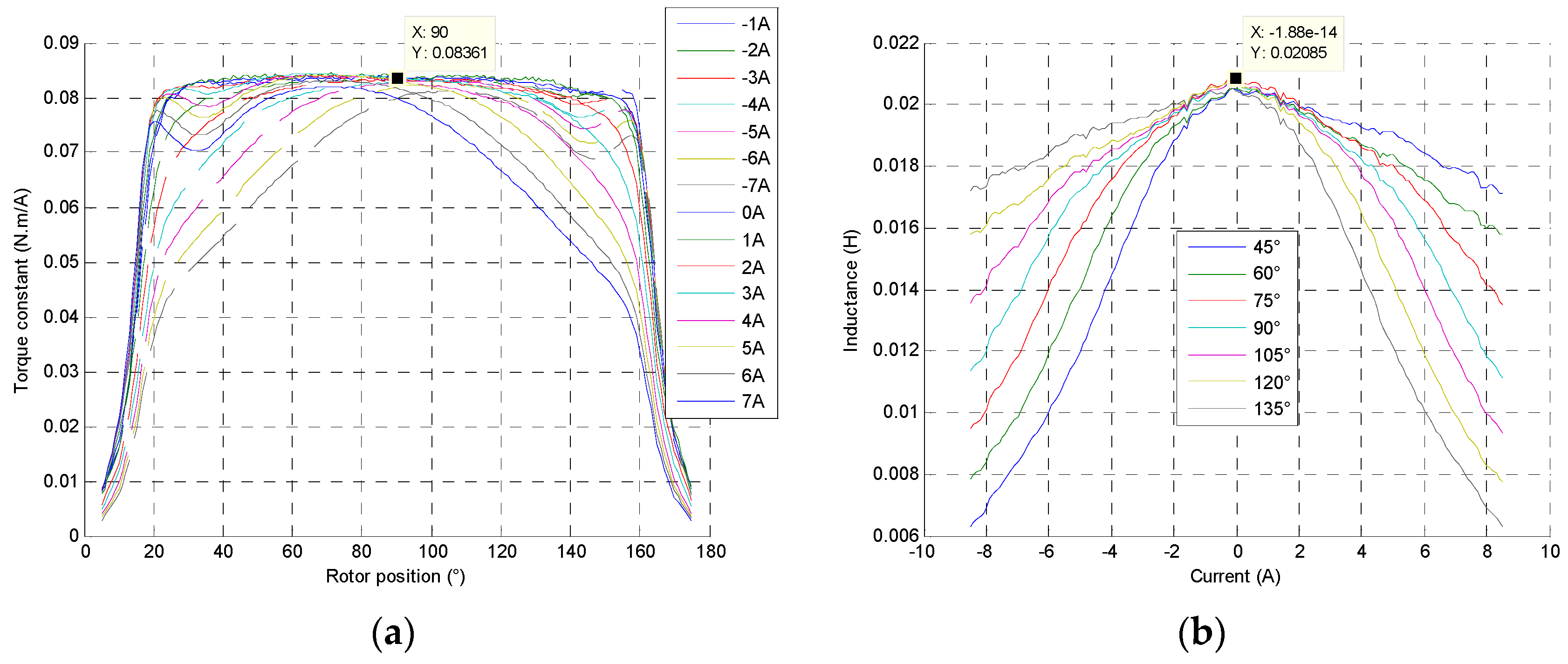
At each rotor position and current, the torques developed by the actuator are measured on a test bench and torque constants can be obtained as shown in Figure 13. At the beginning of a stroke, between 20° and 40°, the actuator torque decreases because of the concentrated windings saturation, and then, at the end of stroke, the core saturation implies naturally the decreasing torque. For positive current, the results give a decreasing torque as the rotor position and current increase. Then, the actuator constant torques can be computed at different currents and rotor positions as shown in Figure 13a at 25 °C.
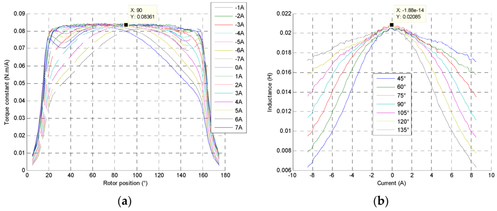
Figure 13.
(a) Constant torque evolution at each rotor position and −7 A to 7 A current of the direct drive actuator at 25 °C; (b) Inductance coil at each rotor position and current.
4.1.2. Non-Linear Inductance
As shown in Figure 13b, the same behavior can be observed in the inductance evolution. Its value decreases as the rotor position and the current increase. The inductance coil values varies according to the core flux density and material saturation level.
4.1.3. Magnetic Hysteresis Influence
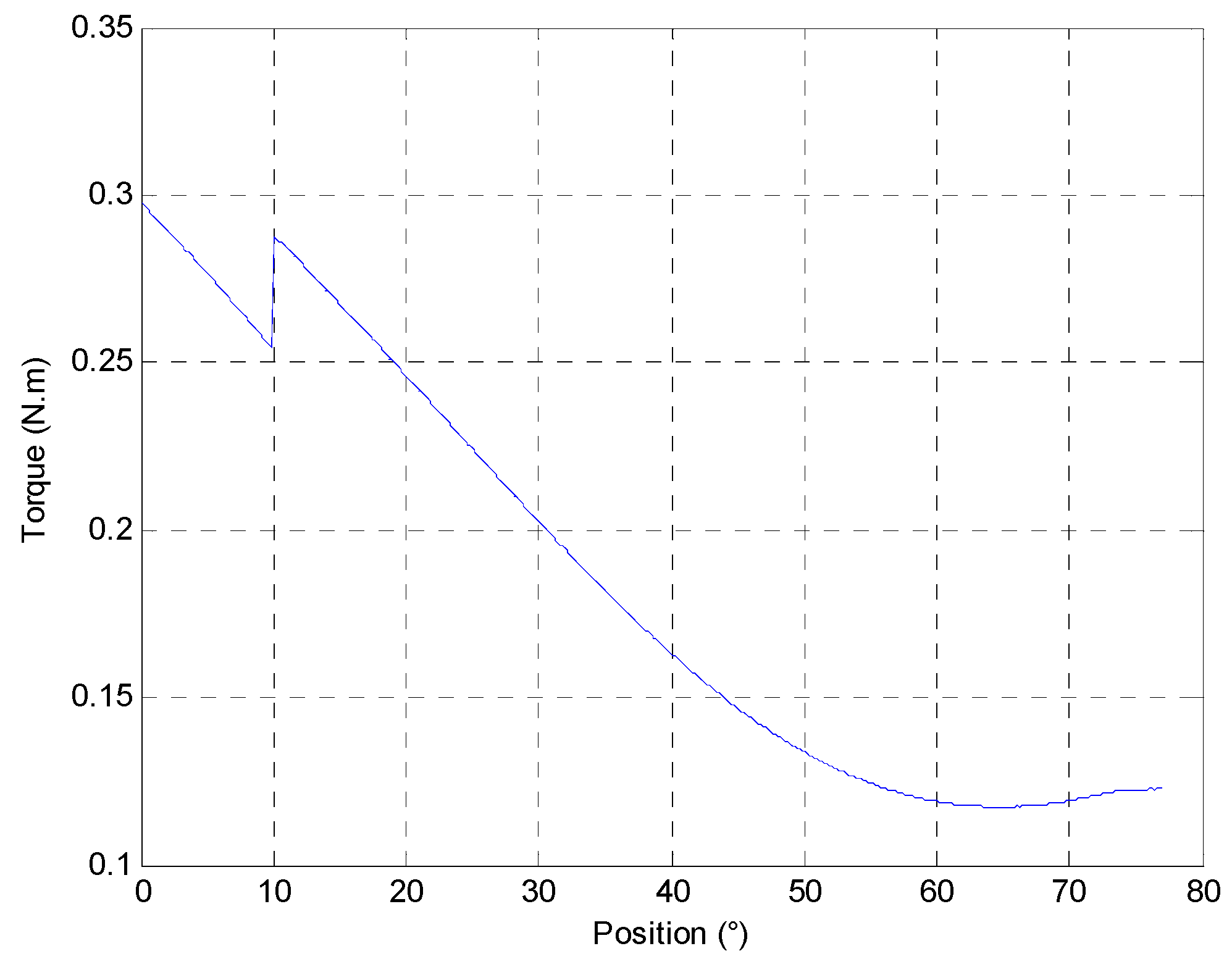
The core is defined by a ferromagnetic material and has a magnetic hysteresis around 100 A/m according to the material manufacturer. A magnetic hysteresis implies a hysteresis torque depending on rotor position such as presented in Figure 14. If the rotor position has to change, the current must be higher than necessary to move the rotor. The B-H hysteresis curve looks like as a memory effect to the electromechanical behavior. The hysteresis torque is variable according the rotor position and the previous position.
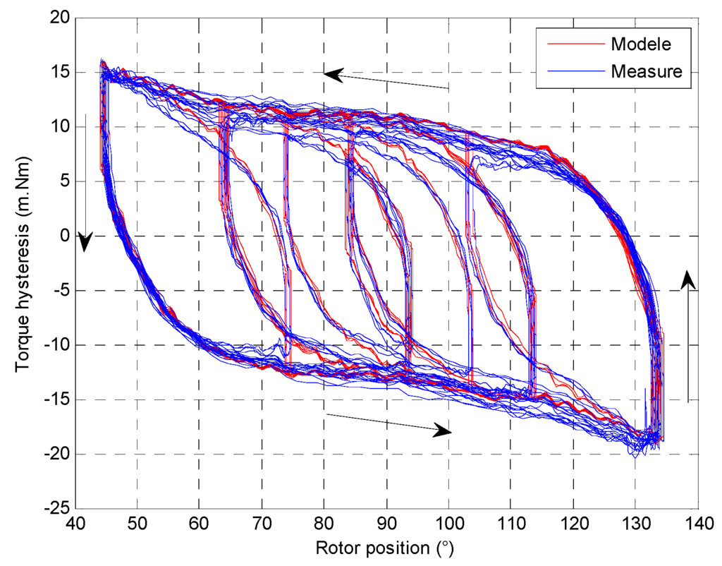
Figure 14.
Hysteresis torque according to rotor position.
To define the electromechanical behavior with non-linearity effects, the actuator is characterized with the torque and current consumption measurements. Then, with Simulink, the electromechanical model use two interpolates tables with inductance, constant torque values and the hysteresis curve.
4.2. Controllers
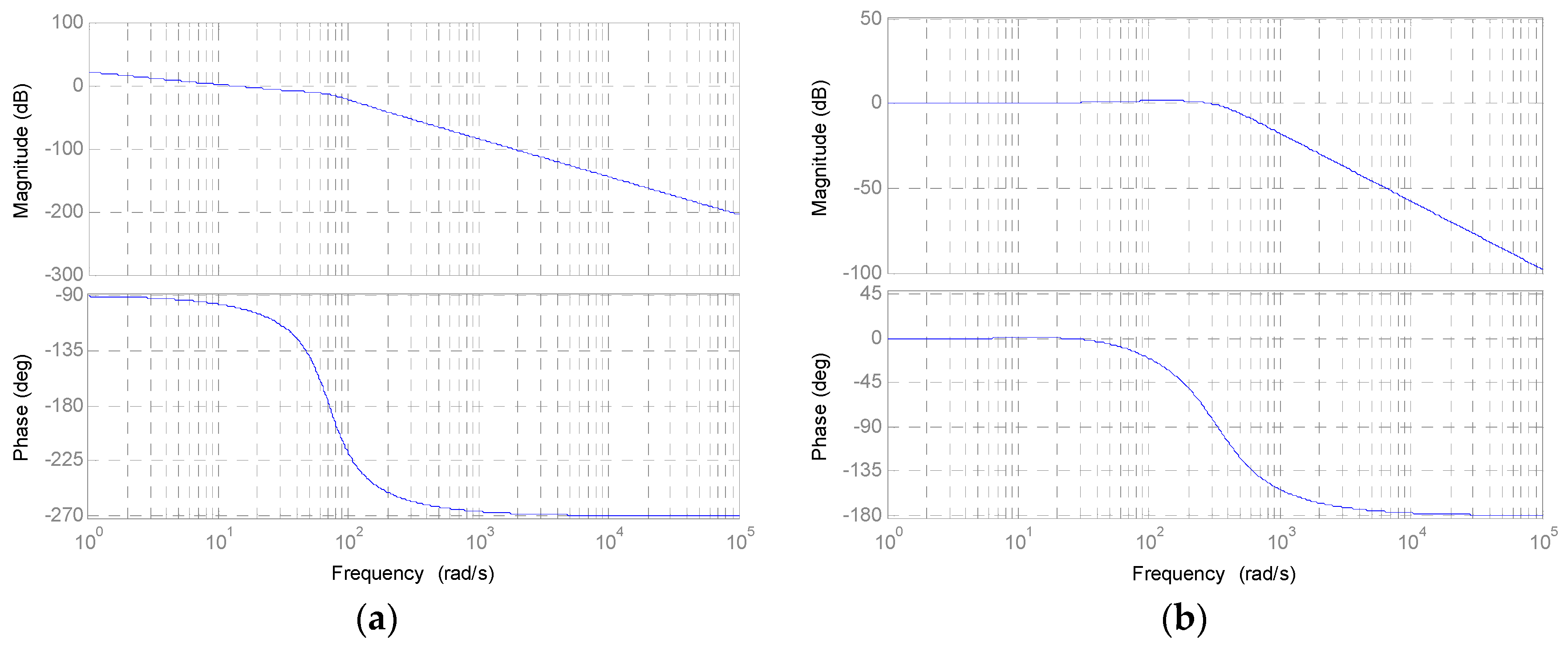
The control law definition is modelized with a linear state space model. In this case, the inductance value involves an electrical time constant (18 ms) of the same order of magnitude as electromechanical time constant (12 ms). The system is considered as a second order system. The direct drive transfer function is defined with nominal parameters:
The system angular frequency ωn value is 71 rad/s. The damping factor ξ value is 0.43, lower than 0.7, highlighting an oscillating system. For this DC machine, a cascade control is defined with two control loops. The primary loop is composed with P controller (with Ki proportional gain) and current measurement. The second loop, devoted to the position control, is defined with PID controller (with Kθ proportional gain, Tθ Integral gain, Dθ Derivative gain) and position measurement.
The transfer function in open loop frequency response is shown in Figure 15a and the closed loop frequency response with controllers in Figure 15b.
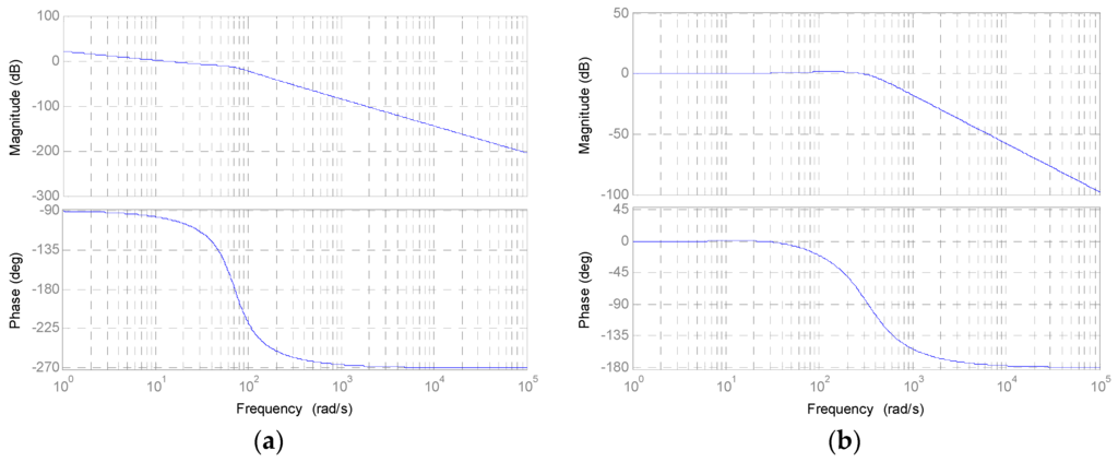
Figure 15.
(a) Open loop frequency response of the direct drive actuator; (b) Closed loop frequency response of the direct drive actuator.
4.3. Dynamic Behavior Measurement and Direct Drive Model
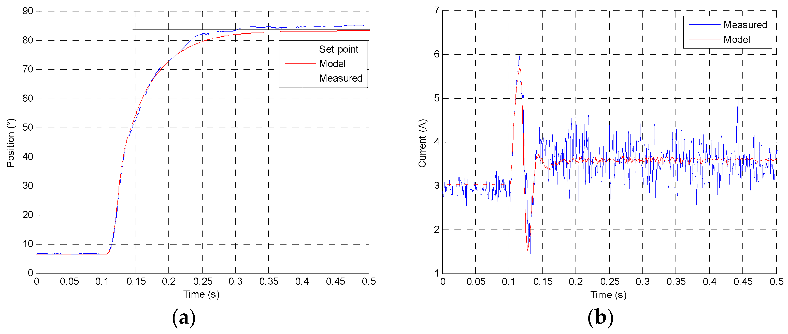
All components are defined according to the previous measurements. The model can be simulated at different set points and different temperatures, supply voltage and charge conditions. For a 77° increasing step, Figure 16a presents the response time at 12 V and 25 °C conditions with 170 mN·m charge, and in Figure 16b the current consumption comparison between the measure and the model is shown.
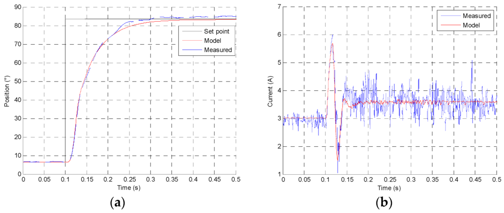
Figure 16.
(a) Position step response comparison between measure and direct drive model; (b) Current response comparison between measure and direct drive model at 12 V and 25 °C conditions.
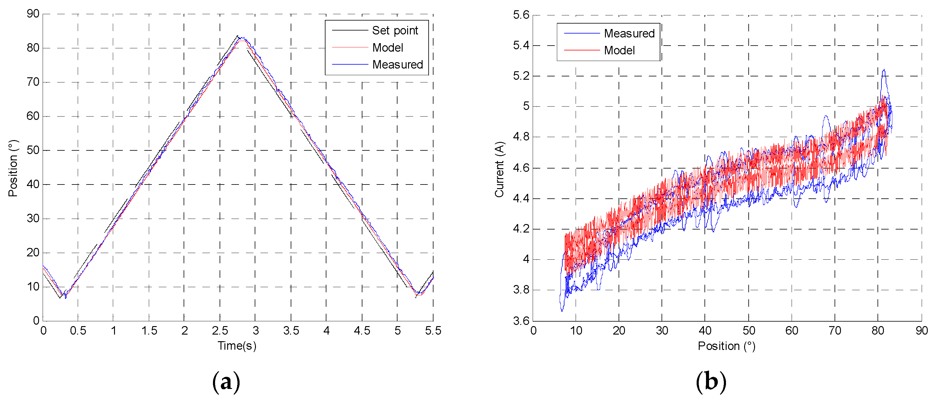
Figure 17a presents the position response of actuator for an increasing and decreasing 77° angular slope at 12 V and 25 °C conditions with 170 mN·m charge. Figure 17b shows the current machine evolution depends of friction and magnetic hysteresis according to the actuator position. A low resistance friction hysteresis can be observed, contrary to an indirect drive actuator.

Figure 17.
(a) Increasing and decreasing slope response comparison between measure and direct drive numerical model; (b) Current response comparison at 12 V and 25 °C conditions.
4.4. Comparative Results between the Optimization and the Prototype
As shown in Table 3, the analytical method offers some sufficient results with a low deviation (<10%) between the numerical model and FEM results and then between the simulation results and the prototype measures.
The difference of rotor inertia values between the prototype and the analytical model is the additional parts to maintain the magnets on the rotor and to connect the actuator on the EGR system.
5. Actuator Energy Consumption with the EGR Load and Position Cycle
The direct drive actuator numerical model is coupled with the EGR system numerical model. Then the complete model is built in order to compute the energy consumption for all conditions of temperature and supply voltage.
5.1. Mechanical EGR System and Actuator Coupling
The actuator and valve system have been described by their electromechanical and dynamic equations. Figure 18 shows a schematic diagram combining the two numerical models. A torsional coupling is added between the actuator and EGR system as described in [17].
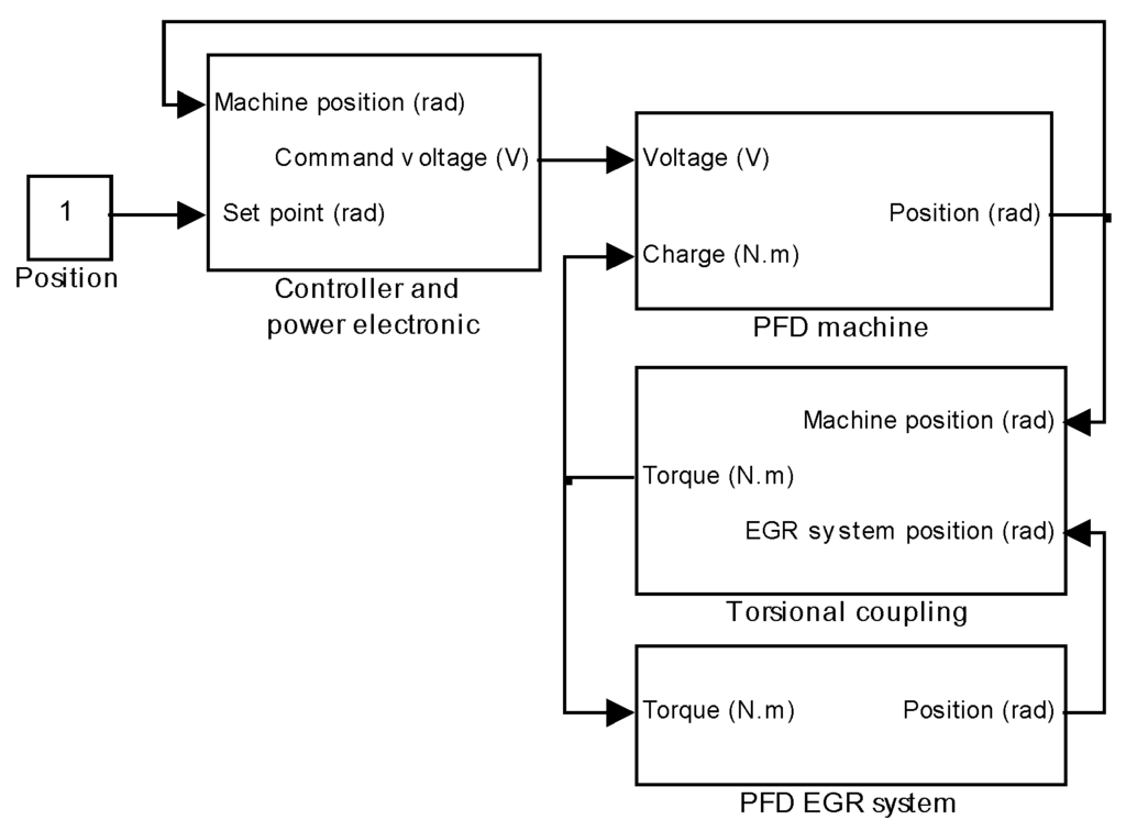
Figure 18.
Actuator and EGR system coupling.
The resistive torque applied on actuator depends on the aerolic system (valve and flap) and the functioning condition of the ICE. The system has a 77° stroke. The worst case is defined by a resistive decreasing torque, as shown in Figure 19.
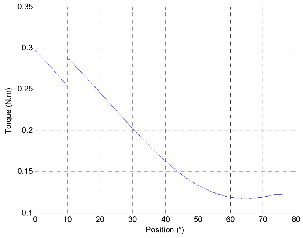
Figure 19.
Load evolution according to the valve and flap position.
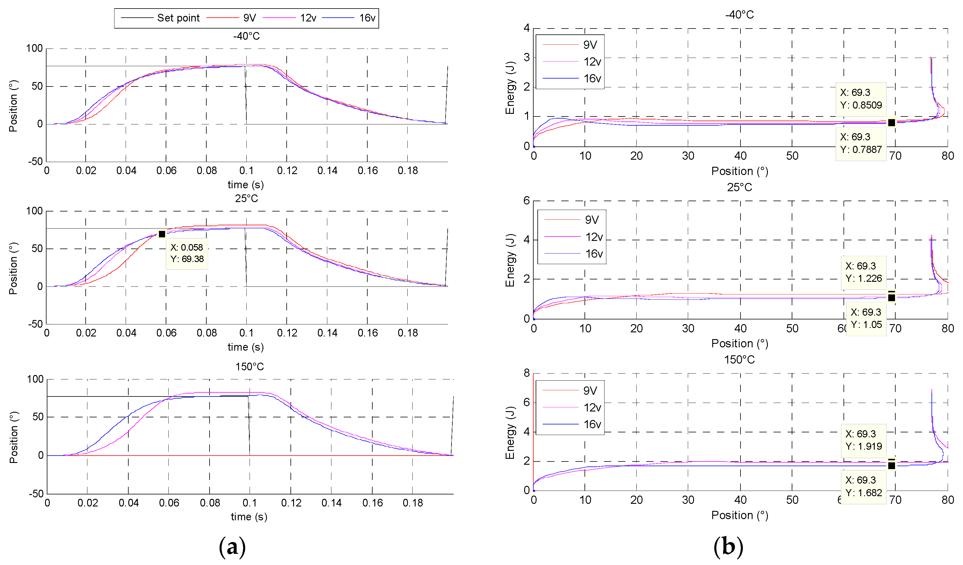
5.2. Increasing and Decreasing Position Step Response
At 12 V and 130 °C, this machine reaches the objective with a 100 ms time response and a satisfactory time response quality. Figure 20a presents the mechanical behaviour in step response and Figure 20b shows the electrical energy for an increasing step. In transient behaviour, the direct drive actuator reaches 69.3° in 58 ms. It consumes 25% of electrical energy to move 90% of stroke and 75% of energy to do the remaining stroke and to keep the position.
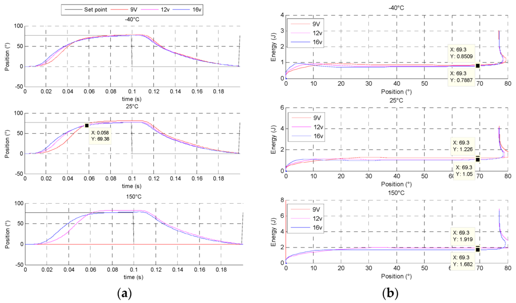
Figure 20.
(a) Increasing and decreasing position step response of direct drive actuator at 25 °C; (b) Electrical energy consumption in increasing position step of direct drive actuator at 25 °C.
The rotor inertia is minimized according to the optimized actuator geometry. This is a major advantage for reducing transient energy consumption. However to maintain the position, the major part of electrical energy is consumed in Joule losses.
5.3. Energy Consumption in 60 s Position EGR Cycle
Figure 21 displays the energy balance of the direct drive with a 60 s position EGR cycle, at different voltage and temperature conditions. All details about the energy balance are given. At 12 V and 25 °C, the direct drive consume a 1300 J electrical energy to realize the 60 s position EGR cycle. Some observations can be explained:
- when the temperature is increased, torque machine decreases according to the remanent flux density of magnets. On the contrary, the electrical resistance of wires increases, so for the same mechanical load level, the system consumes more electrical energy with high temperature level.
- the most of the energy consumption (90%) is dissipated in Joule losses inside the DC machine. The last 10% are mechanical losses inside gears and/or other Joule losses in resistive wire contact and commutation losses in H-bridge.
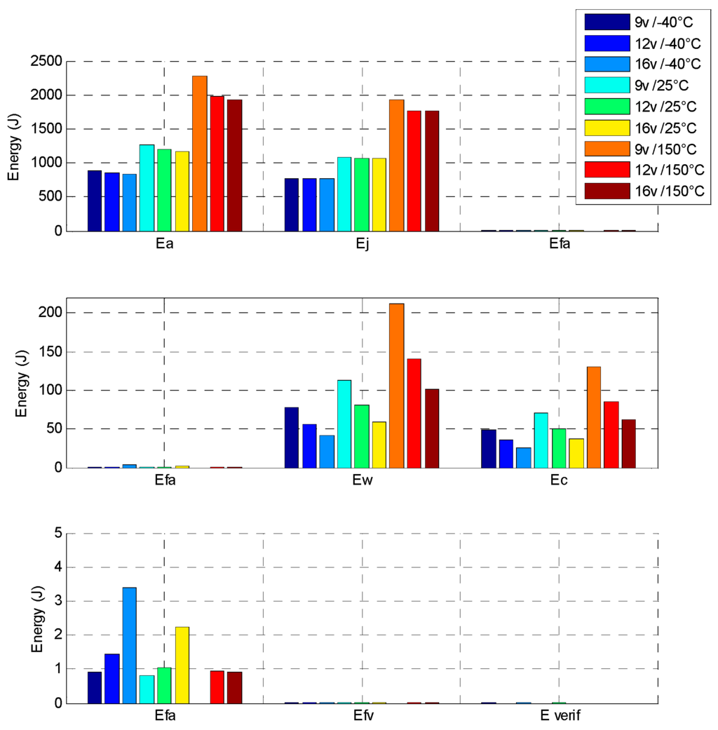
Figure 21.
Direct drive energy balance at different voltages and temperatures. Ea: the electrical energy consumption; Ej: the Joule effect losses; Efa: the actuator mechanical losses; Ew: the wire joule losses; Ec: the H-bridge Joule losses and Efv: the valve mechanical losses.
In order to compare these results, an indirect drive actuator, composed of a brushed DC machine with a spur gears set, is designed and optimized with the same requirements. The indirect drive actuator is simulated with the same conditions as the direct drive described in [7]. This actuator reaches the objective with a 150 ms time response and it cannot go faster. The mechanical behaviour in increasing step response shows that the indirect drive needs 65% of total electrical energy to move 90% of the stroke and 35% of energy for the remaining stroke. The reason for this is that the rotor inertia and the cogging torque are major disadvantages for brushed DC machines, as it leads one to design a strong failsafe spring and as a consequence to increase the transient energy consumption against the spring. Figure 22 shows the energy balance of the indirect drive with the 60 s position EGR cycle, at the same different voltage and temperature conditions.
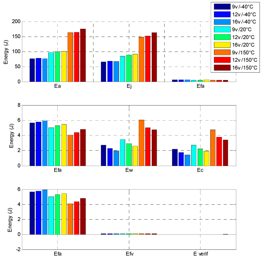
Figure 22.
Indirect drive energy balance at different voltages and temperatures. Ea: the electrical energy consumption; Ej: the Joule effect losses; Efa: the actuator mechanical losses; Ew: the wire joule losses; Ec: the H-bridge Joule losses and Efv: the valve mechanical losses.
The indirect drive actuator need only 100 J electrical energy to realize the 60 s position EGR cycle. The EGR position cycle is dynamically simple and has few requirements to maintain a stable position for a long time.
6. Conclusions
To conclude the study of this prototype, the method of calculation has been proven successful by comparison between the analytical model and the prototype. By the way, it has been demonstrated that the direct drive actuator reached 69.3° in 58 ms in transient behaviour while it consumes 25% of the electrical energy to move 90% of the stroke and 75% of energy to do the remaining stroke and to keep the position. On the other hand, the indirect drive actuator, reaching 69.3° in 120 ms, consumes 65% of the total electrical energy to move 90% of the stroke and 35% of the energy for the remaining stroke. Moreover, in this application, the indirect drive actuator needs only 100 J electrical energy to realize the 60 s position EGR cycle compared to the direct drive which consumes a 1300 J electrical energy. Consequently, in this given case, the EGR position cycle has shown that most part of the cycle has to keep the position and the indirect actuator is better suited for this action. Also, it should be noted that the direct drive would be needed when the applications are faster. This is interesting for ultra-fast and constantly moving applications with a low torque in order to minimize the electrical consumption and for its higher level of reliability. Given the choice of the position cycle of an application, a decision must be made between the choice of a direct or an indirect actuator. It is then important to emphasize the choice of this position cycle.
Author Contributions
Laurent Dufour defined the actuator requirement and contributed to the prototyping, the measurements, and their analysis. Vincent Liebart defined the control law and electronics devices. Christophe Gutfrind was the main author of this article. He has contributed to the actuator design and the analytical and numerical models approaches with Jean-Claude Vannier and Pierre Vidal.
Conflicts of Interest
The authors declare no conflict of interest.
References
- Migaud, J. OCSYGENE 6, Optimization in Air Intake and EGR Systems to Euro 6 Standard and CO2 Reduction. In Proceedings of the SIA International Conference: Diesel Powertrain, Innovative Technologies for Future Emissions Targets, Rouen, France, 5–6 June 2012.
- Wang, J. Air fraction estimation for multiple combustion mode diesel engines with dual-loop EGR systems. In Proceedings of the 46th IEEE Conference on Decision and Control, New Orleans, LA, USA, 12–14 December 2007.
- Iles-Klumpner, D.; Serban, I.; Risticevic, M. Automotive Electrical Actuation Technologies. In Proceedings of the 2006 IEEE Vehicle Power and Propulsion Conference, Windsor, UK, 6–8 September 2006.
- Gutfrind, C. Electromechanical Actuators Optimization Used in Thermal Engine Air Flow Regulation. Ph.D. Thesis, Supelec, Gif-sur-Yvette, France, 11 July 2012. [Google Scholar]
- Kowatari, T.; Tokumoto, S.; Usui, T. Optimization of an Electronic Throttle Control Actuator for gasoline Direct Injection Engines. SAE 1999. [Google Scholar] [CrossRef]
- Automotive DC motors. Available online: http://www.johnsonelectric.com/fr/product-technology/motion/dc-motors/ (accessed on 10 May 2016).
- Gutfrind, C.; Dufour, L.; Liebart, V.; Migaud, J. Energy consumption comparison between two optimized limited motion actuator topologies for an EGR system used in automotive application. In Proceedings of the PCIM Europe 2015 International Exhibition and Conference for Power Electronics, Intelligent Motion, Renewable Energy and Energy Management, Nuremberg, Germany, 19–21 May 2015.
- Bencheikh, N.; Letty, R.L.; Claeyssen, F.; Magnac, G.; Migliorero, G. Limited angle torque actuator for a fine angular positioning. In Proceedings of the 12th International Conference on New Actuators and 6th International Exhibition on Smart Actuators and Drive Systems, Bremen, Germany, 14–16 June 2010.
- Hekmati, P.; Mirsalim, M. Design and analysis of a novel axial-flux slotless limited angle torque motor with trapezoidal cross section for the stator. IEEE Trans. Energy Conv. 2013, 28, 815–822. [Google Scholar] [CrossRef]
- Nasiri-Zarandi, R.; Mirsalim, M.; Cavagnino, A. Analysis, optimization and prototyping of a brushless DC limited angle torque motor with segmented rotor pole tip structure. IEEE Trans. Ind. Electron. 2015, 62, 4985–4993. [Google Scholar] [CrossRef]
- Gutfrind, C.; Dufour, L.; Liebart, V.; Vannier, J.-C.; Vidal, P. Comparative study of limited motion direct drive concepts for automotive applications. In Proceedings of the ISEF Conference, Valence, Spain, 10–12 September 2015.
- Chiang, W.-W. Optimal DC motor design for constant voltage seek motion. IEEE Trans. Energy Conv. 1990, 5, 195–202. [Google Scholar] [CrossRef]
- Skaar, S.E.; Nilssen, R. Genetic Optimization of Electric Machines, a state of Art Study. In Proceedings of the EPE conference NORPIE 2004, Trondheim, Norway, June 14–16 2004.
- BASF. Data Sheet Catamold FeSi3 for Sintered Components. Available online: http://worldaccount.basf.com/wa/NAFTA/Catalog/ChemicalsNAFTA/doc4/BASF/PRD/30046468/.pdf?urn=urn:documentum:eCommerce_sol_EU:09007bb28004768d.pdf (accessed on 10 May 2016).
- CEDRAT FLUX-3D, FLUX 12.0 user guide, Isotropic/ anisotropic soft magnetic material: analytic saturation curve. Available online: https://gate.cedrat.com/j_cedrat/common/portlet/index (accessed on 10 May 2016).
- Hall-effect position sensor technology. Available online: http://www.efiautomotive.com/produ-cts/position-sensors/ (accessed on 10 May 2016).
- Chun, T.-Y.; Hur, G.-Y.; Choi, K.-J.; Woo, H.-W.; Kang, D.-S.; Kim, J.-C. Design of the Aeroload Simulator for the Test of a Small Sized Electro-Mechanical Actuator. In Proceedings of the IEEE International Conference on Control, Automation and System, Seoul, Korea, 17–20 October 2007.


© 2016 by the authors; licensee MDPI, Basel, Switzerland. This article is an open access article distributed under the terms and conditions of the Creative Commons Attribution (CC-BY) license (http://creativecommons.org/licenses/by/4.0/).