
A Novel Method for Proximity Detection of Moving Targets Using a Large-Scale Planar Capacitive Sensor System

Abstract
:1. Introduction
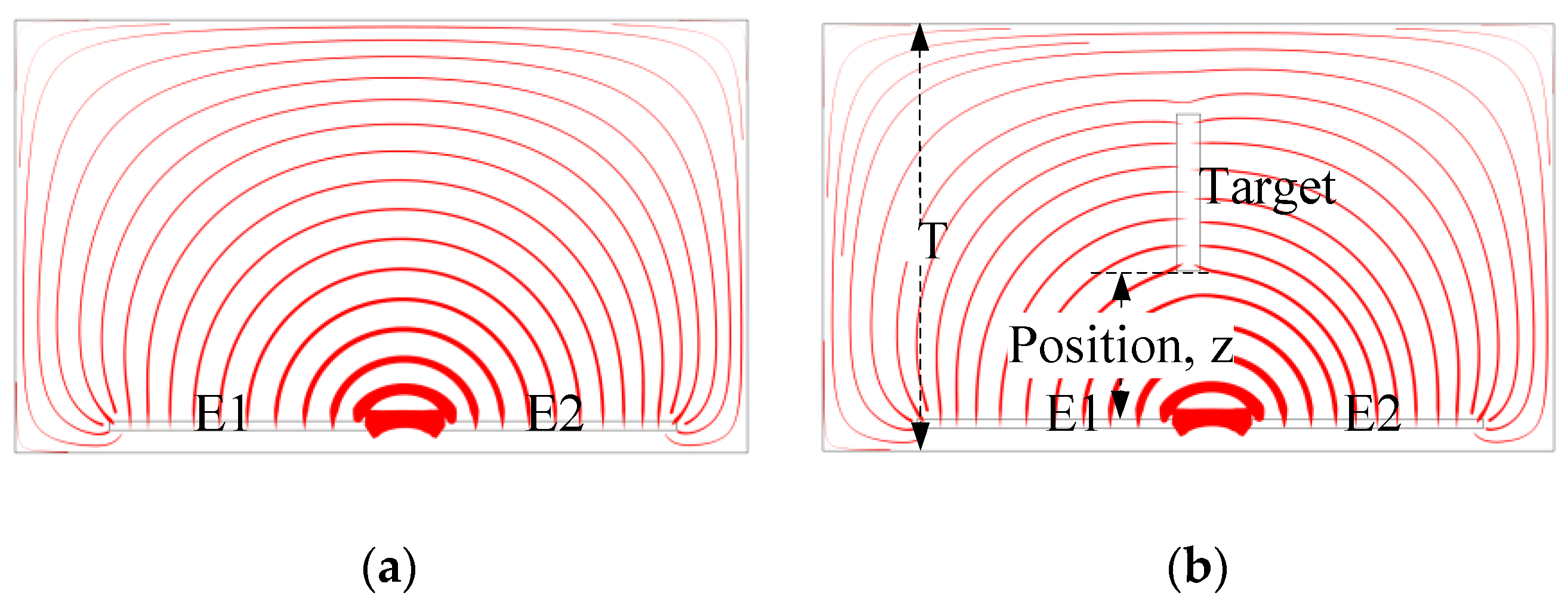
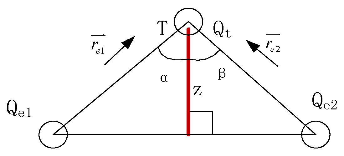
2. Detection Principle
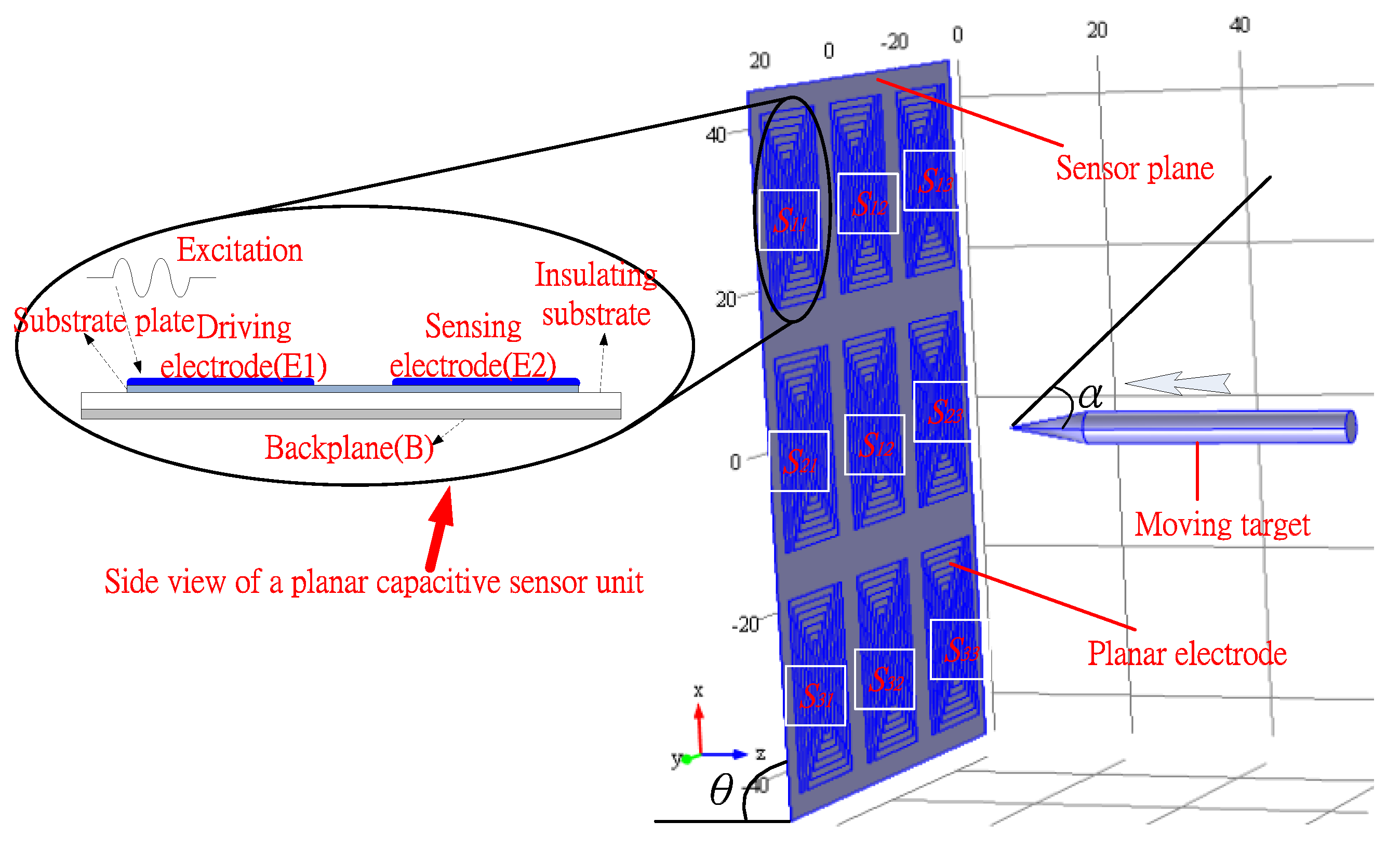
3. Sensor Design
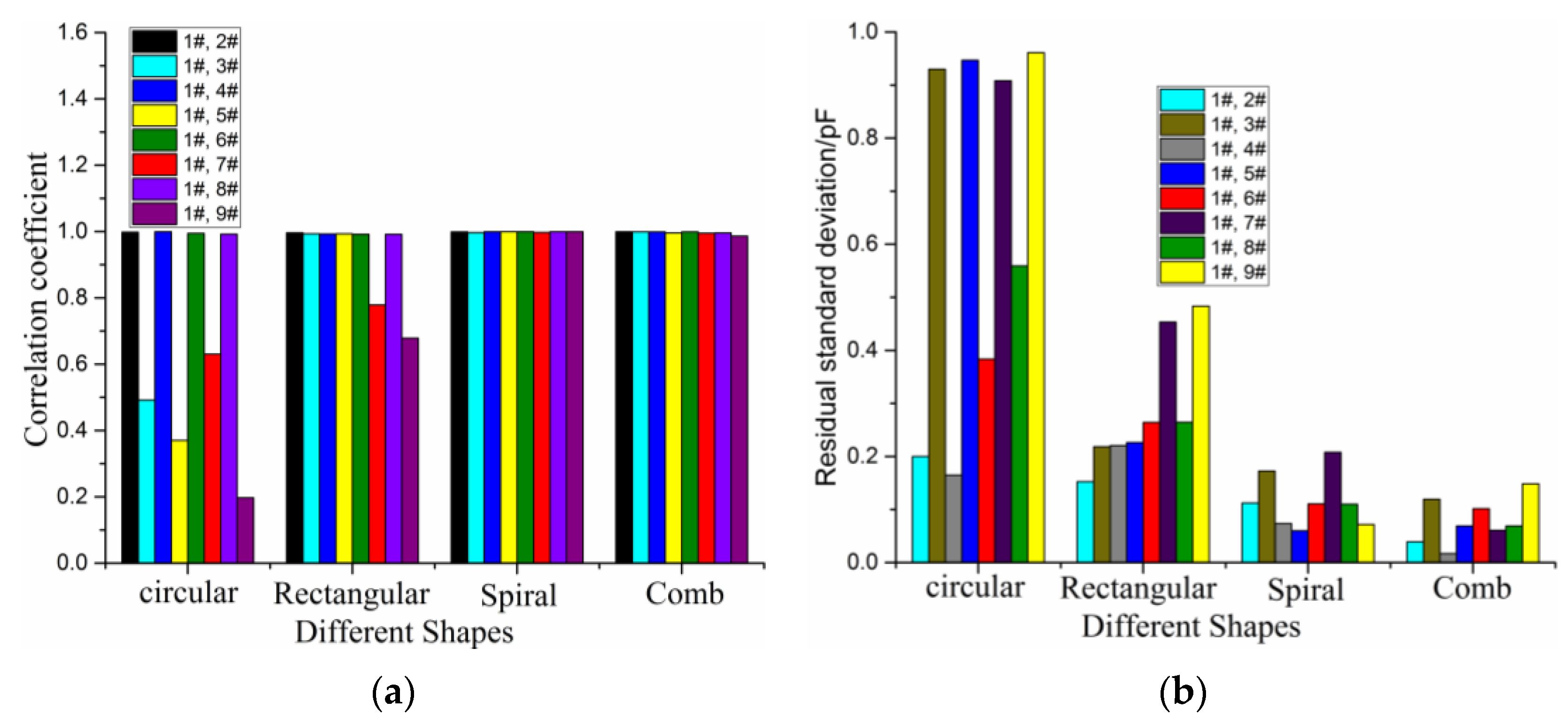
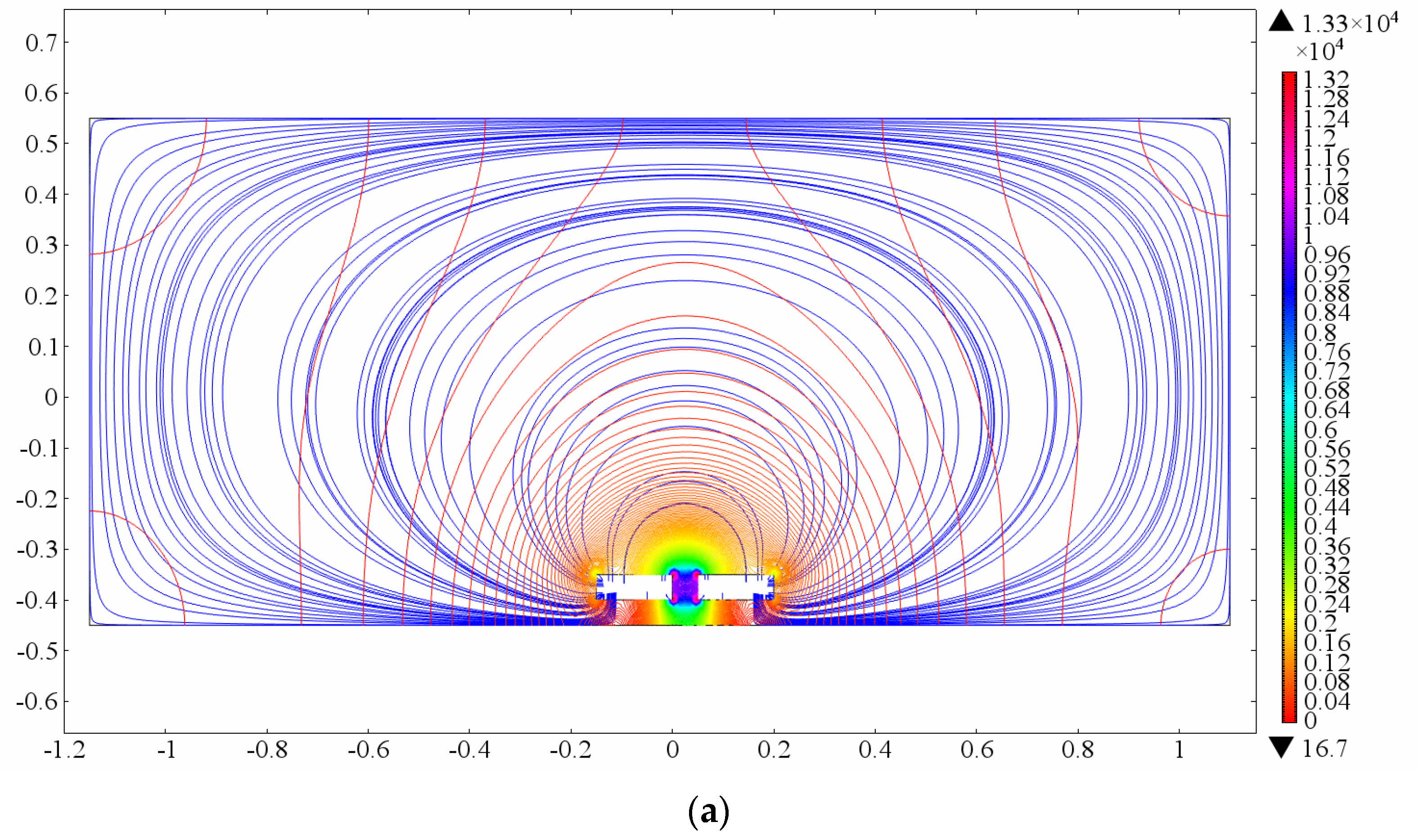
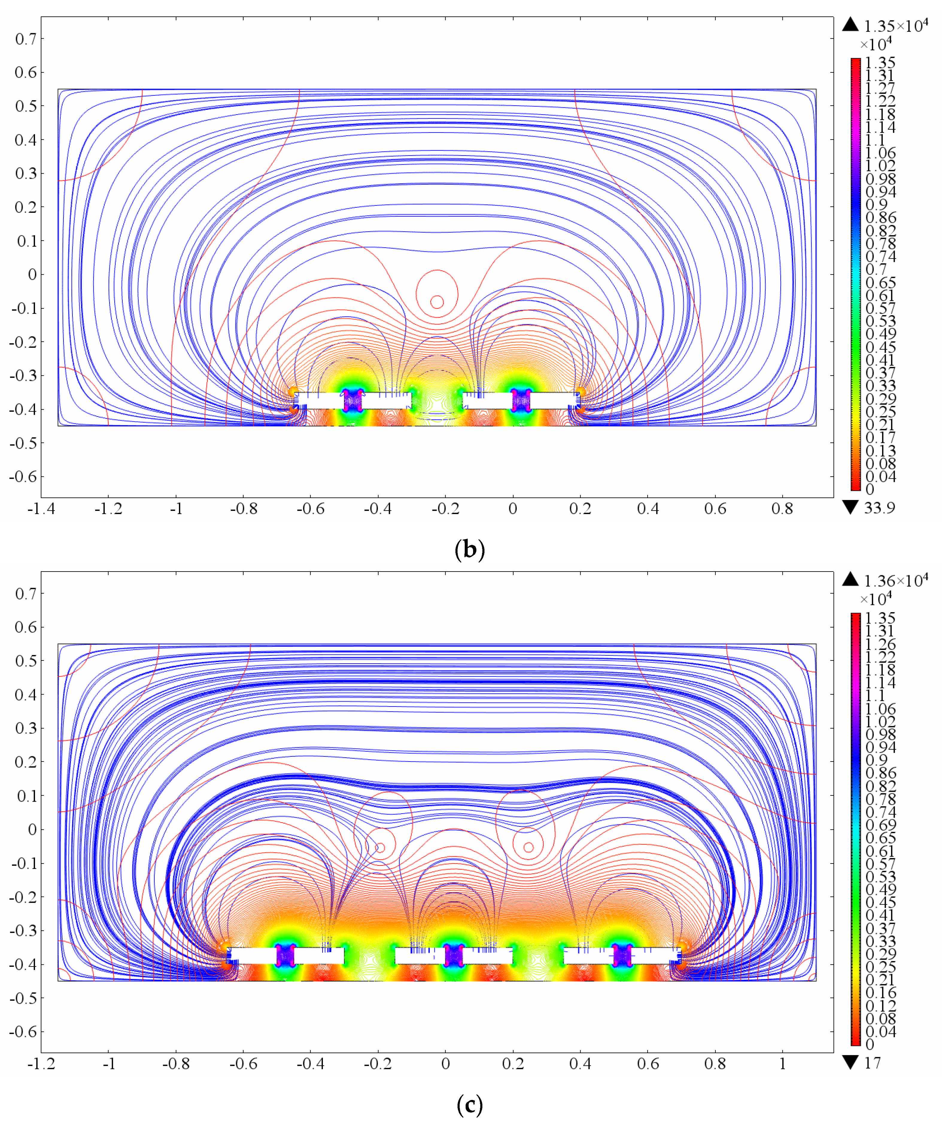
3.1. Sensitivity Distribution of Electrode Shape Design
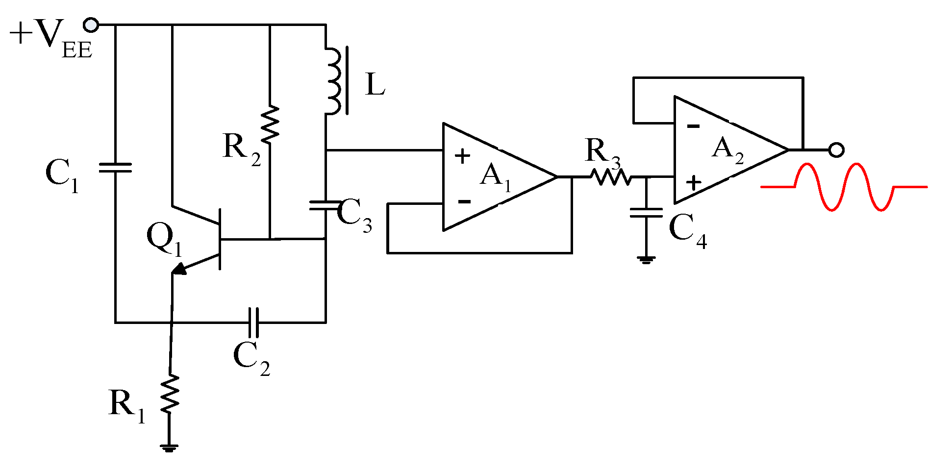
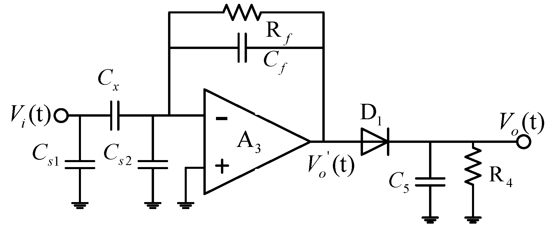
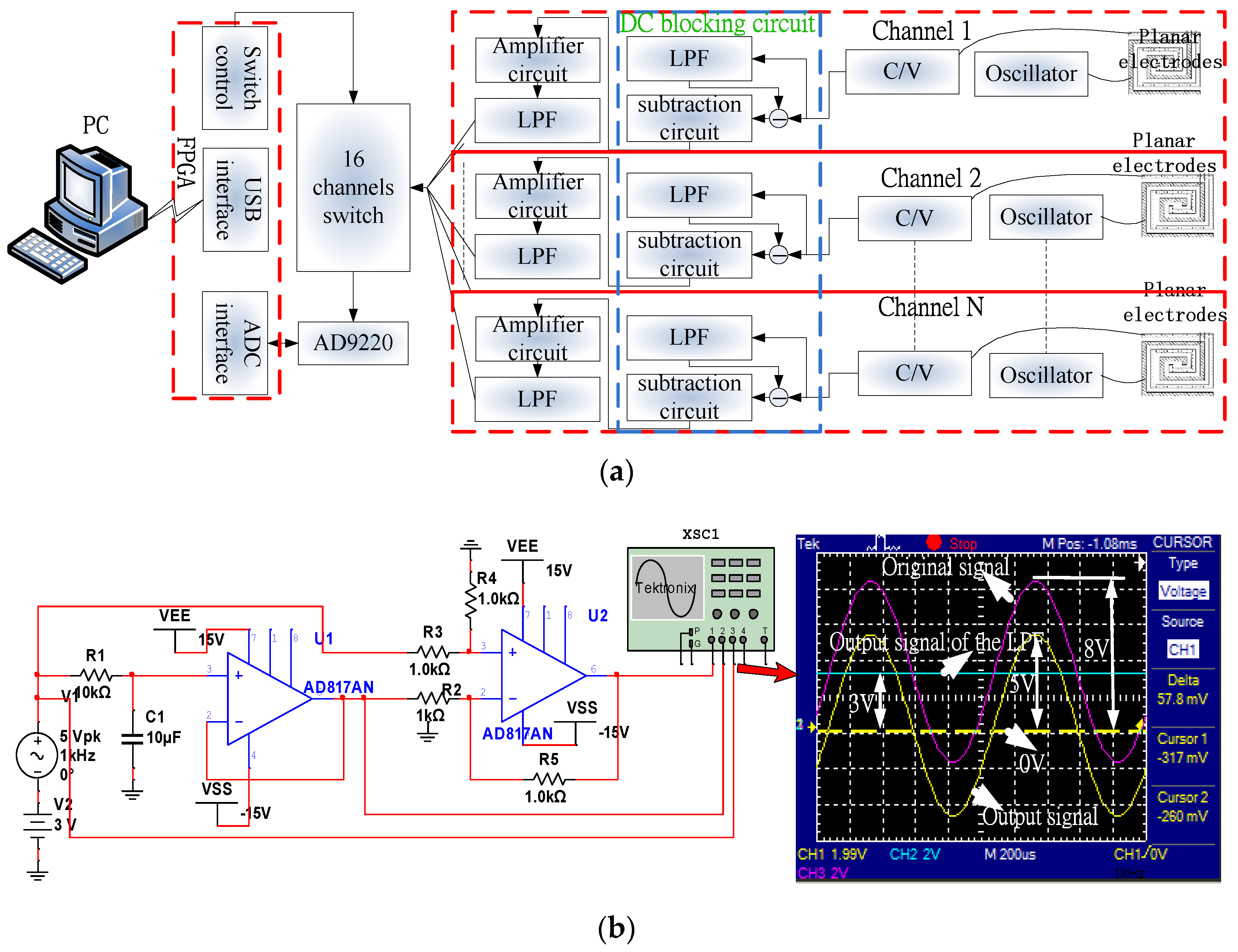
3.2. Driving Excitation and Capacitance Measuring Circuit
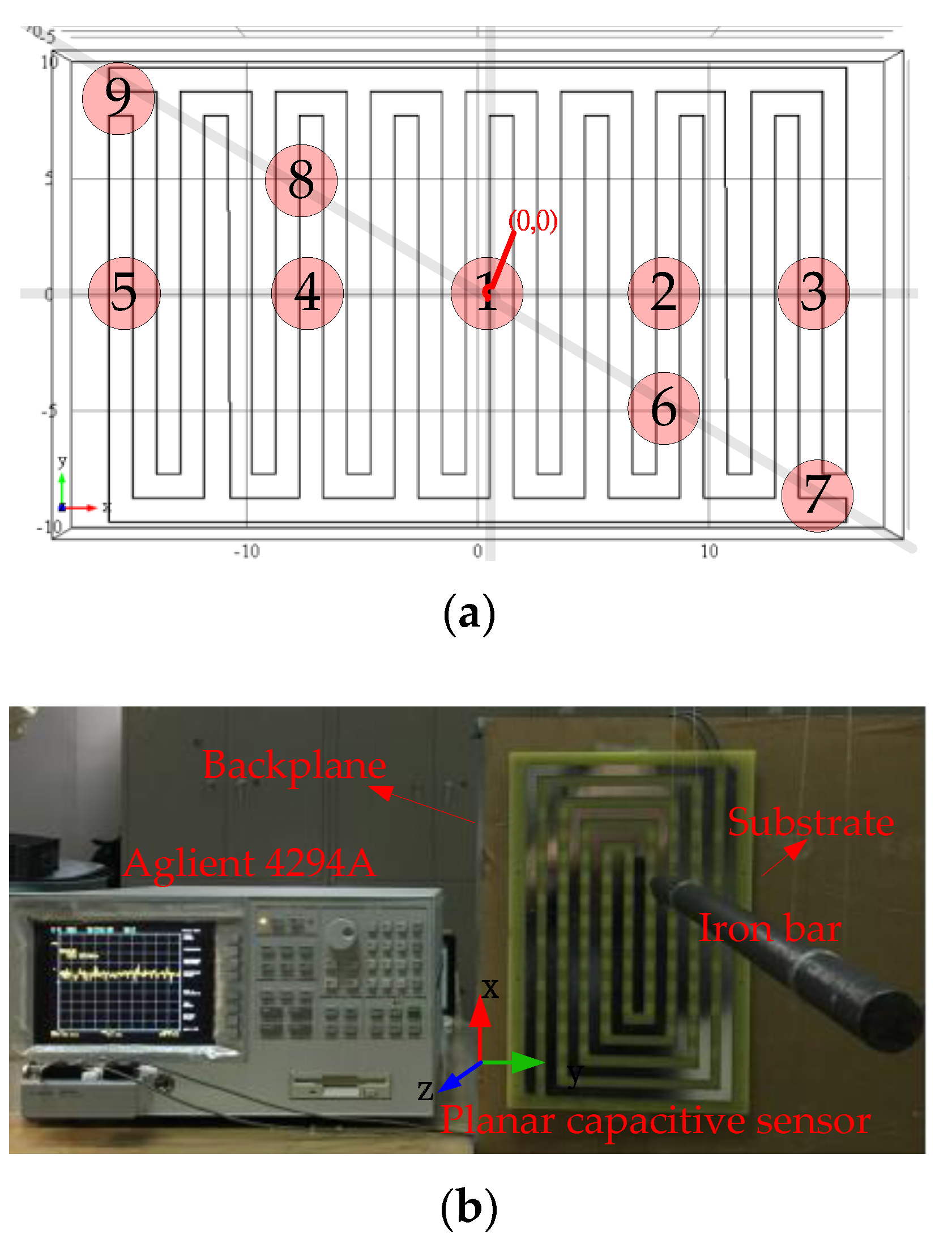
4. Experiments
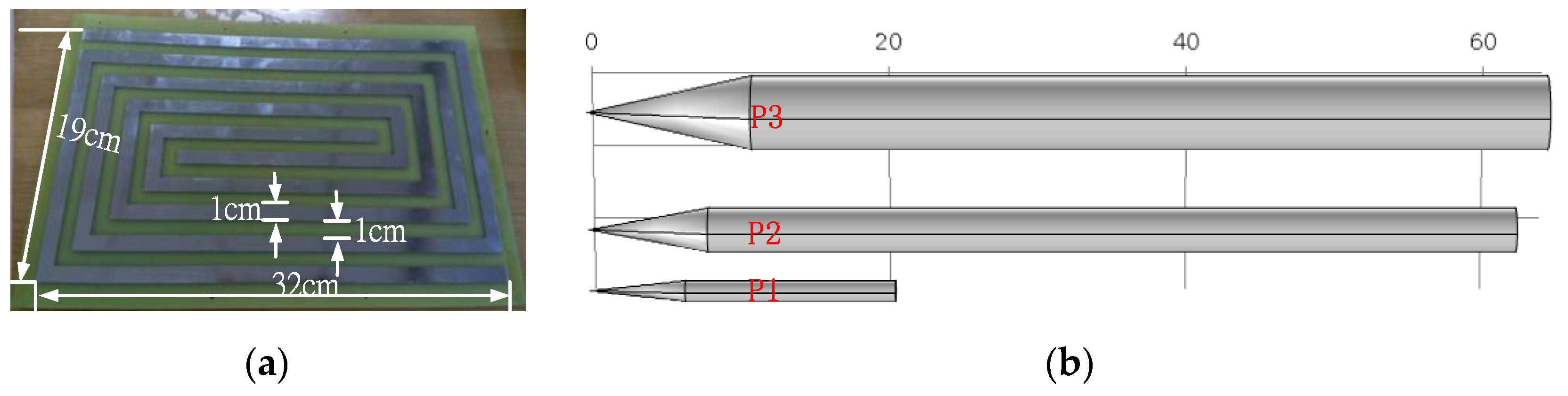
4.1. Experiment Setup
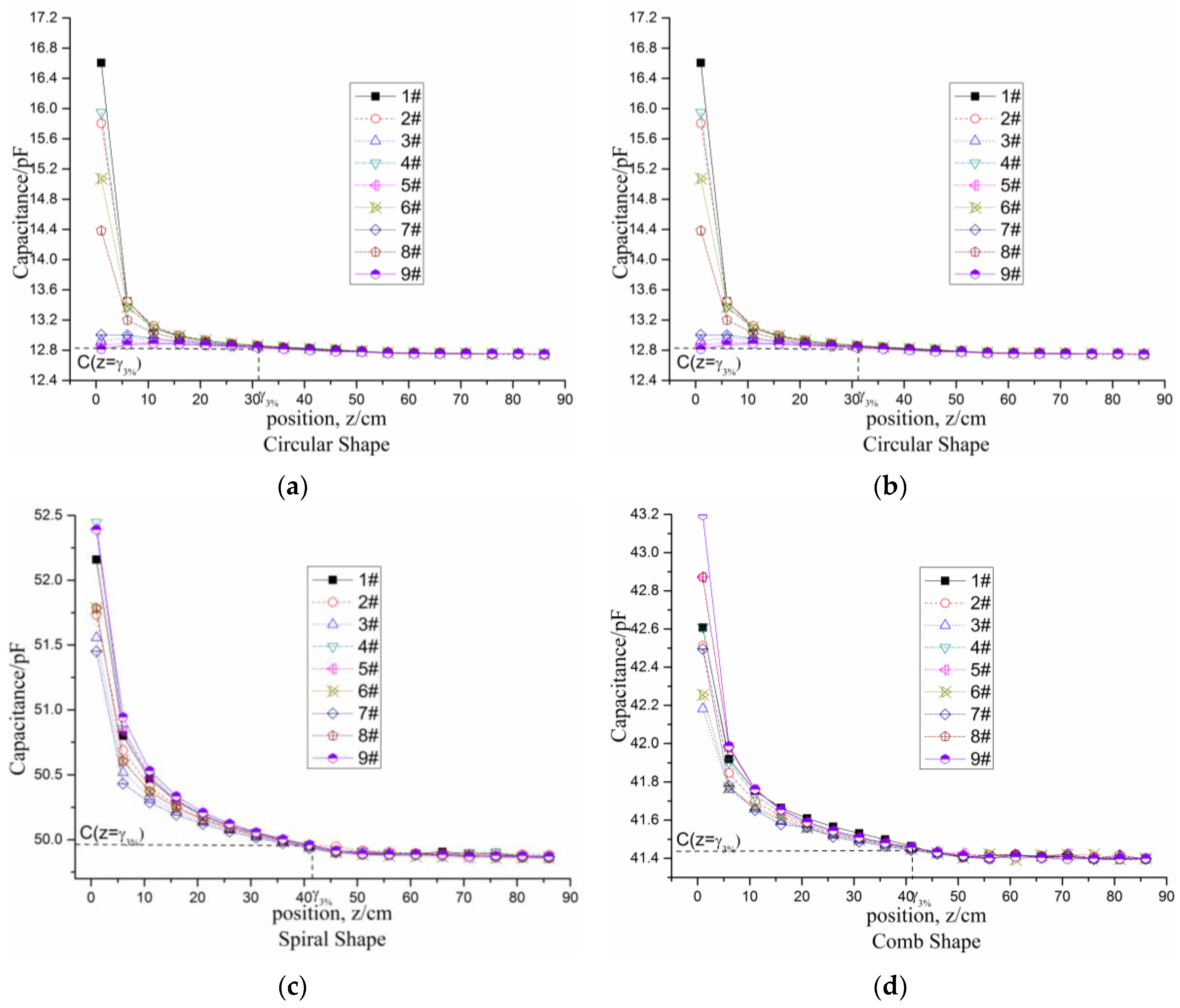
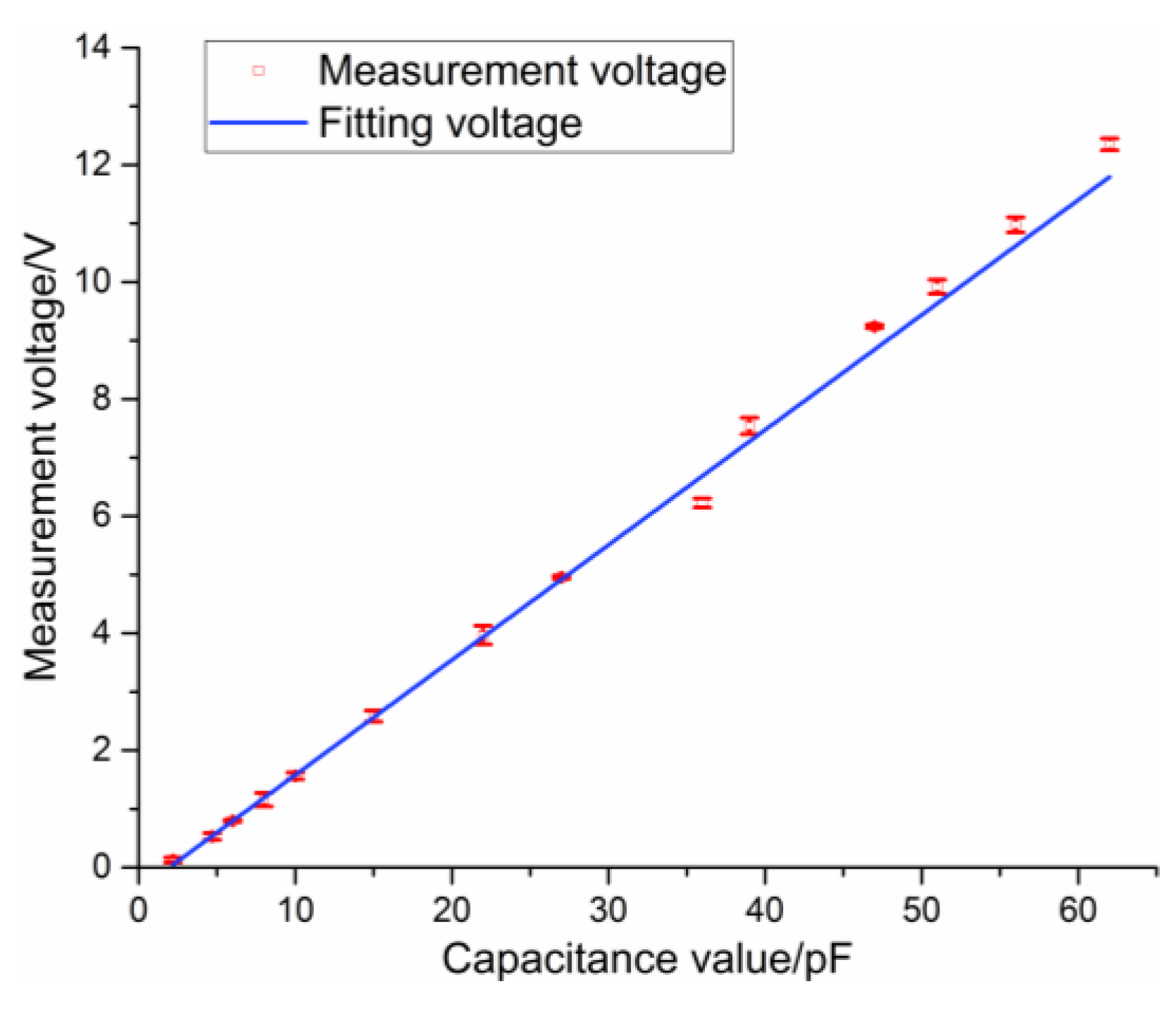
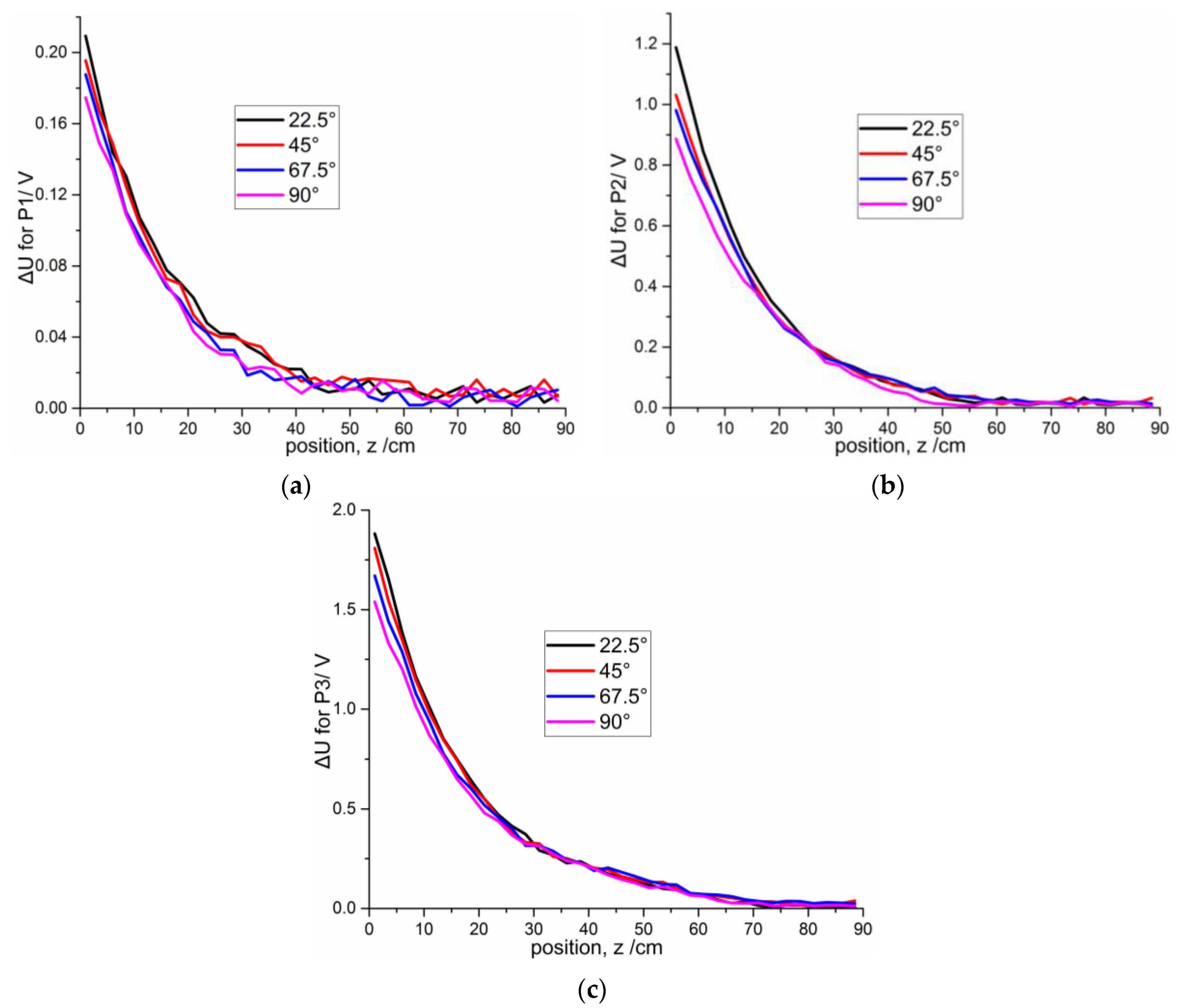
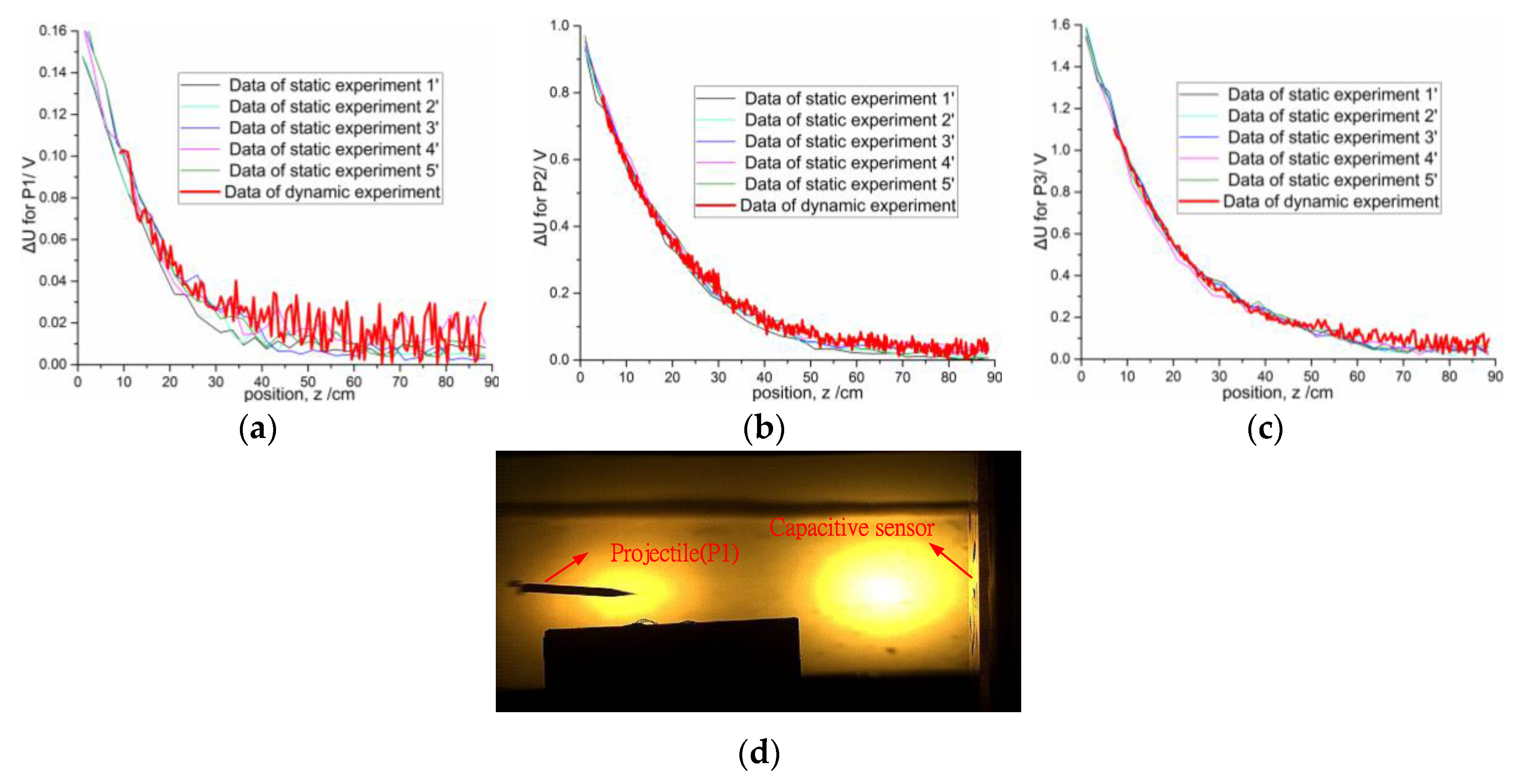
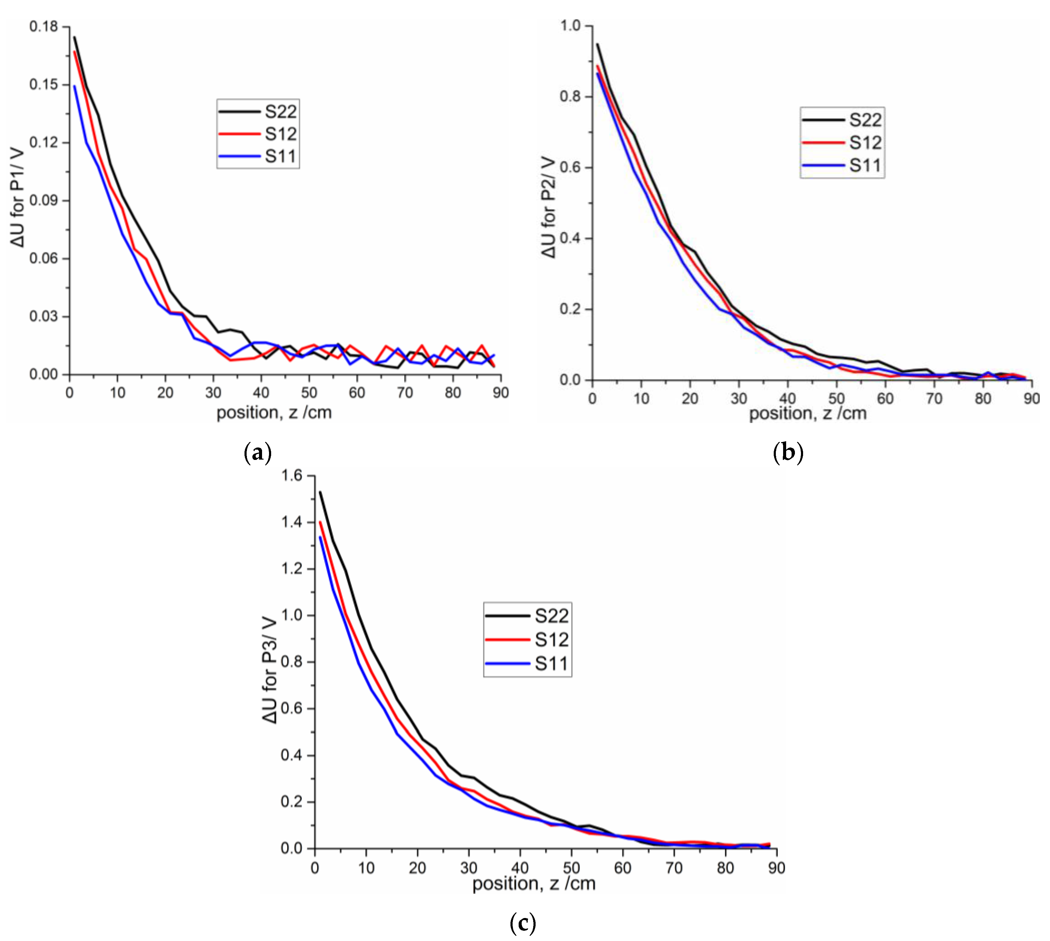
4.2. Experiment Results and Discussion
5. Conclusions
Acknowledgments
Author Contributions
Conflicts of Interest
References
- Hu, X.; Yang, W. Planar capacitive sensors-designs and applications. Sens. Rev. 2010, 30, 24–39. [Google Scholar] [CrossRef]
- Mraović, M.; Muck, T.; Pivar, M.; Trontelj, J.; Pleteršek, A. Humidity Sensors Printed on Recycled Paper and Cardboard. Sensors 2014, 14, 13628–13643. [Google Scholar] [CrossRef] [PubMed]
- Li, J.; Liu, Y.; Tang, M.; Li, J.; Lin, X. Capacitive humidity sensor with a coplanar electrode structure based on anodised porous alumina film. Micro Nano Lett. 2012, 7, 1097–1100. [Google Scholar] [CrossRef]
- Elbuken, C.; Glawdel, T.; Chan, D.; Ren, C.L. Detection of microdroplet size and speed using capacitive sensors. Sens. Actuators A Phys. 2011, 171, 55–62. [Google Scholar] [CrossRef]
- Chen, J.Z.; Darhuber, A.A.; Troian, S.M.; Wagner, S. Capacitive sensing of droplets for microfluidic devices based on thermocapillary actuation. Lab. Chip 2014, 4, 473–480. [Google Scholar] [CrossRef] [PubMed]
- Matiss, I. Multi-element capacitive sensor for non-destructive measurement of the dielectric permittivity and thickness of dielectric plates and shells. NDT E Int. 2014, 66, 99–105. [Google Scholar] [CrossRef]
- Bonilla Riaño, A.; Bannwart, A.C.; Rodriguez, O.M. Film thickness planar sensor in oil-water flow: Prospective study. Sens. Rev. 2014, 35, 200–209. [Google Scholar] [CrossRef]
- Bord, I.; Tardy, P.; Menil, F. Influence of the electrodes configuration on a differential capacitive rain sensor performances. Sens. Actuators B Chem. 2006, 114, 640–645. [Google Scholar] [CrossRef]
- Li, X.; Xu, M. Applied Research on Moisture Content Measurement: One Sided Capacitance Sensors. Meas. Control. 2009, 42, 84–86. [Google Scholar]
- Zhou, Q.; He, W.; Li, S.; Hou, X. Research and Experiments on a Unipolar Capacitive Voltage Sensor. Sensors 2015, 15, 20678–20697. [Google Scholar] [CrossRef] [PubMed]
- Yin, X.; Hutchins, D.A. Non-destructive evaluation of composite materials using a capacitive imaging technique. Compos. Part B 2012, 43, 1282–1292. [Google Scholar] [CrossRef]
- Chen, D.X.; Hu, X.H.; Yang, W.Q. Design of a security screening system with a planar single-electrode capacitance sensor matrix. Meas. Sci. Technol. 2011, 22, 114–126. [Google Scholar] [CrossRef]
- Kirchner, N.; Liu, D.K.; Taha, T.; Paul, G. Capacitive object ranging and material type classifying sensor. In Proceedings of the 8th International Conference on Intelligent Technologies, Sydney, Australia, 12–14 December 2007; pp. 130–135.
- Eidenberger, N.; Zagar, B.G. Capacitive sensor setup for the measurement and tracking of edge angles. In Proceedings of the 2011 5th International Conference on Automation, Robotics and Applications (ICARA), Wellington, New Zealand, 6–8 December 2011; pp. 361–365.
- Kao, T.J.; Newell, J.C.; Saulnier, G.J.; Isaacson, D. Distinguishability of inhomogeneities using planar electrode arrays and different patterns of applied excitation. Physiol. Meas. 2003, 24, 403–411. [Google Scholar] [CrossRef] [PubMed]
- Deng, J.H. Theoretical and Technical Studies on Capacitive Short-Range Target Detection. Ph.D. Thsis, Beijing Institute of Technol, Beijing, China, June 1998. [Google Scholar]
- Li, X.B.; Larson, S.D.; Zyuzin, A.S.; Mamishev, A.V. Design principles for multichannel fringing electric field sensors. IEEE Sens. J. 2006, 6, 434–440. [Google Scholar] [CrossRef]
- Dyakowski, T.; Johansen, G.A.; Hjertaker, B.T.; Sankowski, D.; Mosorov, V.; Wlodarczyk, J. A dual modality tomography system for imaging gas/solids flows. Part Part Syst. Char. 2006, 23, 260–265. [Google Scholar] [CrossRef]
- Sun, J.; Yang, W. Evaluation of fringe effect of electrical resistance tomography sensor. Measurement 2014, 53, 145–160. [Google Scholar] [CrossRef]
- Sun, J.; Yang, W. Fringe effect of electrical capacitance and resistance tomography sensors. Meas. Sci. Technol. 2013, 24, 1–15. [Google Scholar] [CrossRef]
- Ren, Z.; Yang, W. A Miniature Two-Plate Electrical Capacitance Tomography Sensor. IEEE Sens. J. 2015, 15, 3037–3049. [Google Scholar] [CrossRef]
- Yin, X.; Hutchins, D.A.; Chen, G.; Li, W. Investigations into the measurement sensitivity distribution of coplanar capacitive imaging probes. NDT E Int. 2013, 58, 1–9. [Google Scholar] [CrossRef]
- Xu, L.; Sun, S.; Cao, Z.; Yang, W. Performance analysis of a digital capacitance measuring circuit. Rev. Sci. Instrum. 2015, 86, 054703-1–054703-3. [Google Scholar] [CrossRef] [PubMed]


| Electric potential | Electric field | Sensitivity map | |
|---|---|---|---|
| (a) |  |  |  |
| (b) |  |  |  |
| (c) | 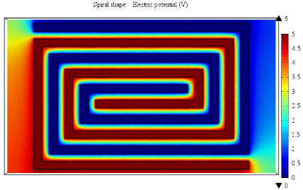 |  |  |
| (d) |  | 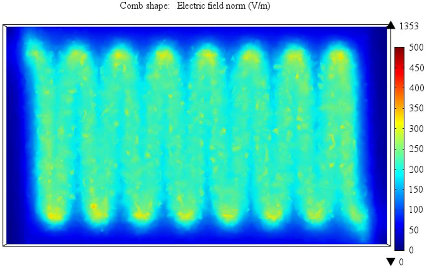 | 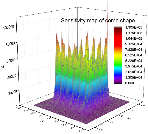 |


| Projectile Structure | P1 | P2 | P3 |
|---|---|---|---|
| Diameter/cm | 5 | 2.8 | 1.4 |
| Length of projectile body/cm | 53 | 54 | 6.5 |
| Length of warhead/cm | 11 | 8 | 14 |
© 2016 by the authors; licensee MDPI, Basel, Switzerland. This article is an open access article distributed under the terms and conditions of the Creative Commons Attribution (CC-BY) license (http://creativecommons.org/licenses/by/4.0/).
Share and Cite
Ye, Y.; Deng, J.; Shen, S.; Hou, Z.; Liu, Y. A Novel Method for Proximity Detection of Moving Targets Using a Large-Scale Planar Capacitive Sensor System. Sensors 2016, 16, 699. https://doi.org/10.3390/s16050699
Ye Y, Deng J, Shen S, Hou Z, Liu Y. A Novel Method for Proximity Detection of Moving Targets Using a Large-Scale Planar Capacitive Sensor System. Sensors. 2016; 16(5):699. https://doi.org/10.3390/s16050699
Chicago/Turabian StyleYe, Yong, Jiahao Deng, Sanmin Shen, Zhuo Hou, and Yuting Liu. 2016. "A Novel Method for Proximity Detection of Moving Targets Using a Large-Scale Planar Capacitive Sensor System" Sensors 16, no. 5: 699. https://doi.org/10.3390/s16050699
APA StyleYe, Y., Deng, J., Shen, S., Hou, Z., & Liu, Y. (2016). A Novel Method for Proximity Detection of Moving Targets Using a Large-Scale Planar Capacitive Sensor System. Sensors, 16(5), 699. https://doi.org/10.3390/s16050699