1. Introduction
As an important type of sensor widely used in the fields of seismological measurement and geography, acceleration sensors hold a significant position in the marketplace. Among all types of acceleration sensors, acceleration sensors equipped with a solid-mass inertial element account for a high proportion. However, for low or ultralow frequency signal measurement applications, acceleration sensors with a solid-mass inertial element are limited by having a more complex structure, low resistance to interference, higher cost and other shortcomings [
1]. Compared to the acceleration sensors equipped with a solid-mass inertial element, a novel microchannel electrochemical sensor (Molecular Electric Transducer, MET) with an electrolytic solution as the liquid-mass inertial element achieves a better performance in the low frequency range field. Electrochemical sensors are used in seismology, seismic exploration, perimeter security systems, structural monitoring [
2], among other applications. In the low frequency domain, a MET offers advantages of higher sensitivity, lower cost, high shock resistance and a wider bandwidth. An in-depth study on the use of METs to measure low frequency vibration signals is necessary. Generally, a MET consists of a reaction cavity, an external conditioning circuit and a protective shell. As the core element in the MET, the reaction cavity, filled with electrolyte, with the reversible reaction
ensures the sensing of a vibration signal [
3]. In addition, both sides of the reaction cavity are encapsulated by two elastic membranes that influence the dynamic response of the MET.
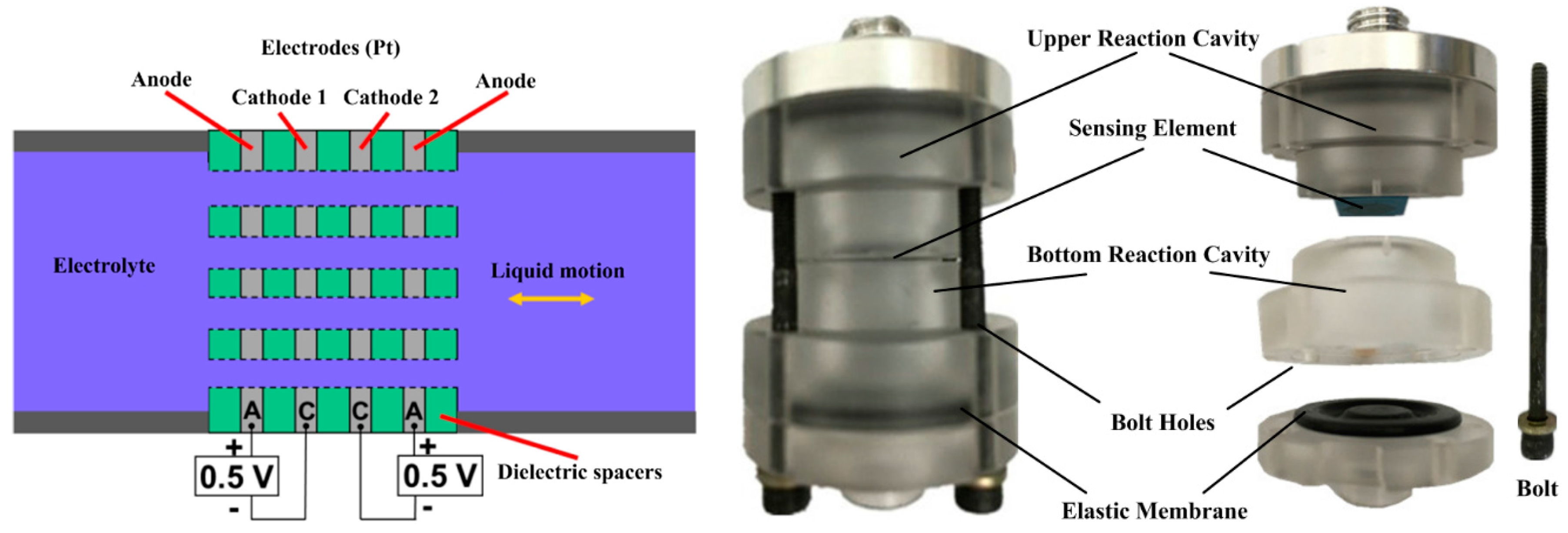
Figure 1 presents the basic concept of the MET and consists of two anode-cathode pairs [
1]. The multichannel structure immersed in the electrolyte allows the liquid flow to move inertially, with four electrodes arranged in the order of anode-cathode-cathode-anode (ACCA), which are separated by dielectric layers. The electrolyte is capable of flowing in and out of the multichannel through the electrodes. The usual method to bond the membrane to the reaction cavity is to apply the four-bolt structure shown in
Figure 1 (right), thus preventing liquid leakage.
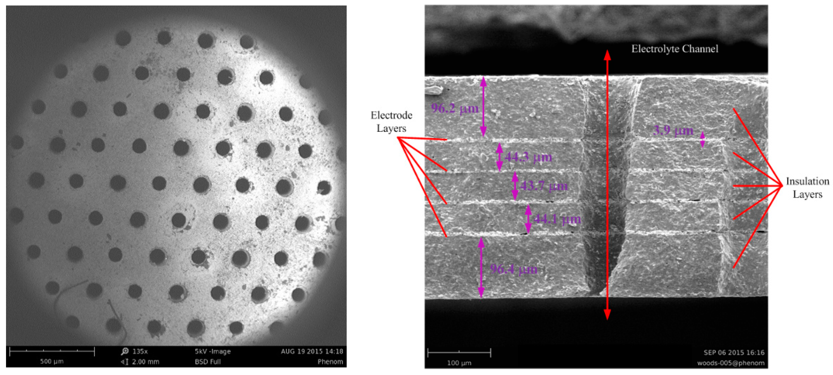
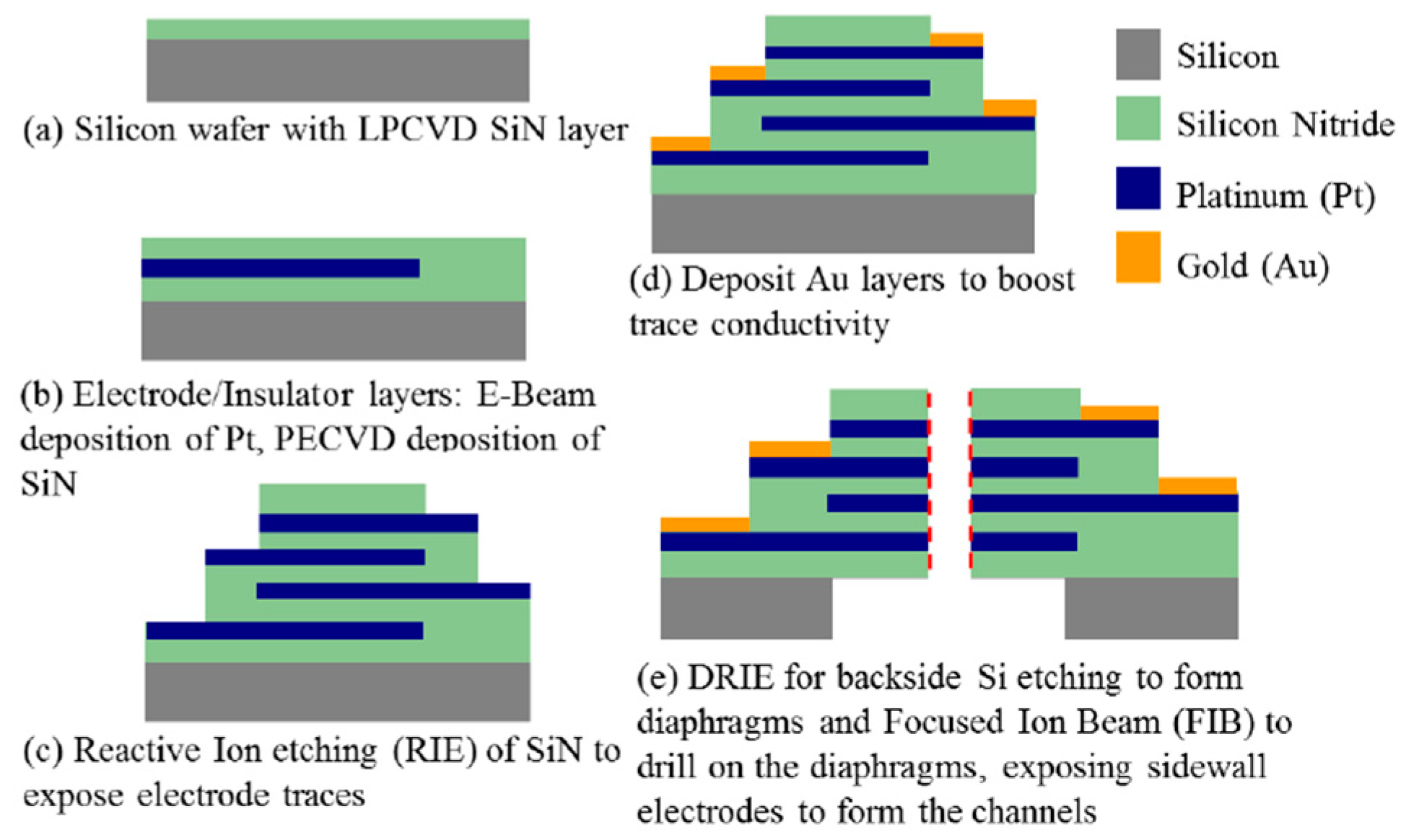
A sensing element with microflow channels (
Figure 2) is found in the middle of the reaction cavity. Alternately overlapping platinum layers (four) and insulating layers (five) are obtained by a procedure of bonding, pressuring and puncturing by Low Temperature Cofired Ceramic (LTCC) technology (
Figure 3).
In the sensing element, due to the fact the external vibration signal and the multichannel are oriented in the same direction, the electrolyte flow changes with the measured vibration signal when the MET is in the working condition. Because the MET is an active sensor, a fixed electric potential difference imposed alternately on the platinum layers is arranged as anode-cathode-cathode-anode (ACCA). With the reversible reaction
on the interface of the cathodes, a miniature electrochemical system is created in the cavity of the MET [
1]. When the electrolyte shows ion movement caused by external vibration excitation, a concentration gradient of the electrolyte is generated in the whole reaction cavity, especially on the electrodes in the sensing element. Meanwhile, the enhanced effect of electrode kinetics controls the rate of the electrochemical reaction. Thus, the changing current density derived from the reversible electrochemical reaction on the surface of the electrodes is proportional to the signal from the external vibration. Thus, the differential current generated by two cathodes, which is the source of the MET output, can be the output from the cathodes after amplification by the conditioning circuit because the interface charge transfer is associated with the generation and absorption of the tri-iodide ions on the electrode surface. Therefore, the electrical current through any electrode can be related to the flux of active ions towards or away from the electrode, according to the following equation:
where D is the diffusion coefficient, c is the concentration of the active charge carriers, q is the charge transferred across the interface in single electrochemical reaction,
n is a unit vector normal to the surface of the electrode, and integration is performed over S, the electrode surface area.
The operating principle of MET can be described as follows: when an electric voltage is applied to the electrodes, an electrochemical (background) current appears. When an external vibration appears, the electrolyte starts moving due to inertia, and the convective transport of ions changes the electrode current according to the mechanism described above. The difference in the cathode currents in the two anode-cathode pairs is used as the MET output signal. Although each electrode current is non-linear with respect to the fluid velocity, the combined output of both cathodes is linear for a very wide range of fluid velocities. The MET output current is given by [
3]:
where
and
are the currents through the surface of the corresponding cathodes, and
and
are the surface areas of the corresponding cathodes.
The optimization of the design of the MET requires too many physical parameters of the complex electrochemical process to be obtained directly from practical measurement. Under practical conditions, due to the different materials, manufacturing processes, experimental conditions and other issues, many variables such as flow field distribution in the reaction cavity, a variety of charging ion concentration gradients and the electrode surface ion concentration, etc., cannot always be measured directly by practical experiments, so a few problems of the MET cannot be solved by traditional methods.
Recently, with the development of numerical simulation technology, multiphysics finite element analysis methods can process the joint simulation of a complex electrochemical and microfluidic model. Combined with the traditional methods, the use of numerical simulation aids in the development of a comprehensive analysis of the study of METs. Since 2010, many numerical simulation models have provided effective solutions in the relevant MET study fields. Because the study of the MET combines electrochemical, electrical, microfluidic and other complex multiphysics aspects, this study takes advantage of the current new simulation technology methods to accomplish the modelling of the study object. With the numerical simulation, physical characteristics that could not be measured and observed before in the practical experiments can be studied effectively. Beginning in 2012, based on numerical simulation and practical experiments, Sun [
4,
5], Vadim [
6,
7,
8] and Huang [
1,
9,
10] have studied the theory and the complex electrochemical changes in the MET reaction cavity. By combining the results of practical experiments with numerical simulations, a number of performance optimizations can be accomplished by analysing the actual results measured by data acquisition equipment and the simulations that involve effective concentrations of charged ions and comprehensive velocity-field distributions.
Compared with traditional acceleration sensors, its special structure and measurement principles make the MET an effective transition from a solid inertial element to a liquid inertial element due to a great innovation. With its special inertial element, unique advantages for vibration signal measurement in the low frequency domain can be achieved. For the MET, new methods have become available to guarantee its measurement accuracy.
First, the elastic membrane element in the MET causes the electrolyte to be encapsulated in the reaction cavity. When an external excitation signal arrives, the liquid inertial element not only generates a movement in the same direction as the vibration direction but also generates a movement in the perpendicular direction, and a trend in the flow is followed. Under normal conditions, the electrolyte should remain in a state of standard laminar flow in the reaction cavity. However, due to the kinetic energy caused by the high frequency or large amplitude of the external vibration signal, a slip happens between the layers of the electrolyte that is exposed to laminar flow. When the electrolyte is moving, to prevent the electrolyte from generating a series of slips between the laminar layers, the elastic membranes that are positioned on both ends of the reaction cavity are capable of maintaining the laminar flow of the electrolyte under various forms of external vibration motion. Only if the laminar flow state is maintained, will the MET be operated under the best performance conditions.
According to the theory mentioned above, the elastic force generated by the elastic membrane can control the movement of the electrolyte in the reaction cavity. When an external vibration occurs, the electrolyte in the reaction cavity of the MET moves in the same way as the vibration signal. Thus, the electrochemical current signal that acts as the source of the output of the MET is proportional to the vibration intensity on the cathodes. The elastic membrane element has the main function of adjusting the electrolyte motion. However, for different measurement fields, the design of the elastic membrane influences the dynamic response of the MET. To compensate and decrease the negative impact caused by improper design, in this paper, a novel elastic membrane design method that can adapt to the different structures of the MET is proposed. Combining the practical size of the MET with numerical modelling, the state of movement of the electrolyte in the reaction cavity and elastic membranes with different thicknesses can be observed by the multiphysics finite element method. With the same pulse signal imposed on two METs with different elastic membranes, a series of evaluations can be accomplished. The optimal design of the elastic membrane can be calculated by comparing variables such as the response time. In addition, in this paper, relevant practical experiments are also applied to verify the correctness of the numerical simulation. Finally, amplitude-frequency and phase-frequency characteristics are discussed to describe the influence of different membranes on the MET.
2. Mathematical Modelling
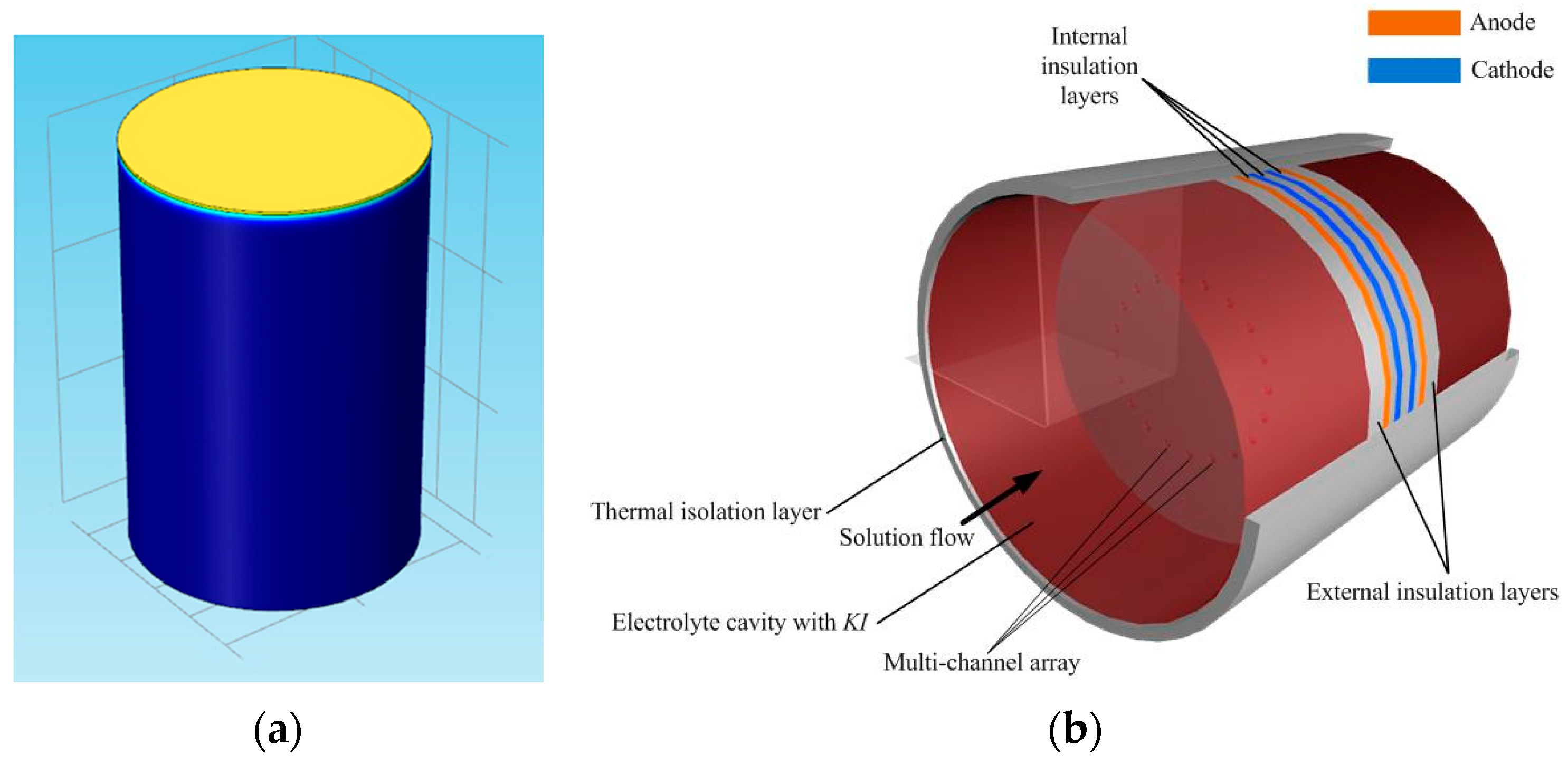
The geometric structure of the MET is built as shown in
Figure 4 (left). The elastic membrane element (yellow) is placed on the top of the cavity. The reaction cavity is marked as blue. The inside structure is presented in
Figure 4 (right). The membrane element is on the top of the numerical model. In the simulation, a Gaussian pulse response signal is used as the external vibration excitation. By observing the movement state of the electrolyte in the reaction cavity and the elastic membrane, the dynamic response characteristics of the membrane can be calculated by the numerical simulation.
The numerical simulation parameters of the dimensions and materials are shown in
Table 1.
Navier-Stokes equations are applied to build the fluid dynamic model of the electrolyte as follows:
where
v and
t denote the velocity of the electrolyte flow and time. The electrolyte density is
.
P, a scalar, represents the pressure, and
μ = 1.4 × 10
–3 Pa is the dynamic viscosity. Parameter
a is the acceleration of the external signal.
In this study, Gauss’s law is applied to demonstrate charge conservation:
where
,
and
are the permittivity (F·m
–1), potential (V) and charge density (C·m
–3), respectively.
In addition, the Nernst-Plank-Poisson equation is used to describe the mass transport (Equations (6) and (7)) subject to mass continuity (Equation (8)). Because of the high degree of nonlinearity, multiple length and time scales are observed, and the applicable approximation, which applies to scales larger than nanometres, is the assumption of electroneutrality (Equation (7)) [
11]:
where
is the flux of species
i (mol·m
–2·s
–1) and
Di is the diffusion coefficient of species
i (m
2·s
–1). Here we set
DI– =
DK+ = 2.8 × 10
–9 m
2·s
–1 and
DI3– = 2.0 × 10
–9 m
2·s
–1.
ci is the concentration of species
i (mol·m
–3),
zi is the charge number of species
i;
mi is the mobility of species
i (m
2·V
–1·s
–1),
is the velocity vector (m·s
–1), and
Ri is the mass source of species
i (mol·m
–3·s
–1).
Assuming electroneutrality and small absolute concentration gradients of charge-carrying electrolyte species, the electrolyte current obeys Ohm’s law (Equation (9)) subject to a constant conductivity (Equation (10)). Meanwhile, the concentration of the electrolyte is effectively infinite, Fick’s 2nd law for an incompressible flow is applied (Equation (11)) as follows:
where
is the conductivity (S·m
–1), Q is the charge source (A·m
–3·), and F is the Faraday constant.
Combining the equations from Equation (6) to Equation (11), the partial differential equations (PDEs) are applied in the Comsol Multiphysics software as shown below [
3]:
In addition, the Butler-Volmer condition is set up to convey the procedure of electrode kinetics:
where
n is the out-normal of the electrode surface, and
are the anodic and cathodic reaction constants, respectively. The parameter α is the charge transfer coefficient for the cathodic reaction and is set to 0.5 in this study. U = 0.8 V is the imposed electric potential at the electrodes, and E
0 = 0.54 V is the equilibrium potential.
Instead of applying the shell interface, which is barely coupled with the hydrodynamic model of the electrolyte in the cavity, extensive efforts were made to build a suitable solid-liquid interface, which was inspired by tracking the immiscible fluid-fluid interface. The membrane model offered by the structural mechanics of Comsol Multiphysics can be coupled with the modified Navier-Stokes equations, including the surface tension force [
11,
12]. To be the input to the stress load interface of the membrane model, the surface tension force is imposed on the membrane in the vertical direction. According to the relationship between stress and train yields to the constraints such as linear elastic condition and solid material setting, the force distribution on the membrane in the traverse direction is also capable of being calculated. As a feedback effect from the membrane to the electrolyte, the movement state of the electrolyte in the reaction cavity can be influenced, corresponding to the movement state of the membrane. Therefore, variables such as velocity and force distribution for both electrolyte and membrane can be solved by the finite element analysis method.
The topology of the solid-liquid interface changes with time for the contact interface of the solid elastic membrane and the electrolyte. The level set method as well as the phase field method are both well suited for modelling moving boundaries where topology changes occur [
13]. Both methods are available in the CFD module and the structure mechanics model. In this solid-liquid two phase model, the level set function determines the solid-fluid interface by tracing the isolines of the level set function,
Φ. The equation governing the transport and initialization of
Φ is:
where
u is the fluid velocity, and γ (m/s) and ε (m) are the initialization parameters. The ε parameter determines the thickness of the membrane around the interface where
Φ goes from zero to one. When stabilization is used for the level set equation, we can typically use an interface with a thickness of ε =
hc/2 to describe the initial membrane, where
hc is the characteristic mesh size in the region encompassed by the solid-liquid interface. A suitable value for γ is the magnitude of the maximum velocity occurring in the model. Because the level set function is a smooth step function, it is also used to determine the density and dynamic viscosity globally by:
Here
ρl,
μl,
ρm and
μm denote the constant density and viscosity of the electrolyte and the membrane, respectively [
11]:
In Equation (18), ρ represents the density (kg/m3) of the electrolyte, and u is the velocity (m/s). The parameters t and p are time (s) and pressure (Pa), respectively. The momentum equations contain gravity, ρg, and the surface tension force is also denoted by .
The surface tension force in Equation (16)
is defined by:
where
is the surface tension coefficient,
I is the identity matrix,
n is the interface unit normal, and
is a Dirac delta function. The interface normal is calculated from:
The level set parameter
is also used to approximate the delta function by a smooth function defined by [
13]:
when the surface tension force
is confirmed by using the stress and strain interface of the membrane model, the surface tension force is proportional to the stress in the vertical direction. Constrained by the material setting and the relationship between stress and strain in the membrane model, the elastic force generated in the transverse direction is also calculated.
The constraints and boundary conditions are described as follows: the bottom of the cavity uses no-slip conditions, u = 0. The sidewall of the cavity surrounding the electrolyte uses the wetted wall as its boundary condition. The centre axis of the cylinder cavity corresponds to the symmetry boundary condition. For the membrane constraints, the outer edge of the membrane is supported in the transverse direction and the edge connecting the membrane with the sidewall is set as a fixed constraint. To summize the modelling process, a modified Navier-Stokes equation based on the principles of a two phase flow is presented to describe the state of the movement of the electrolyte. Meanwhile, the surface tension force at the solid-liquid surface is derived by the modified Navier-Stokes equation. To strongly couple the liquid phase with the solid phase, the surface tension force acts as the input of the stress force in the membrane model. Due to the elastic material setting and the stress-strain relationship of a membrane structure, the force distribution on the membrane will be solved integrally. As the feedback from the solid phase to liquid phase, the force and velocity change would correspondingly affect the movement state of the electrolyte. With the constraints and the boundary conditions mentioned above, the level set function is applied to describe the solid-liquid interface. Coupling the membrane with the electrolyte tightly also makes effective communication between the electrolyte and the membrane by the variable velocity.
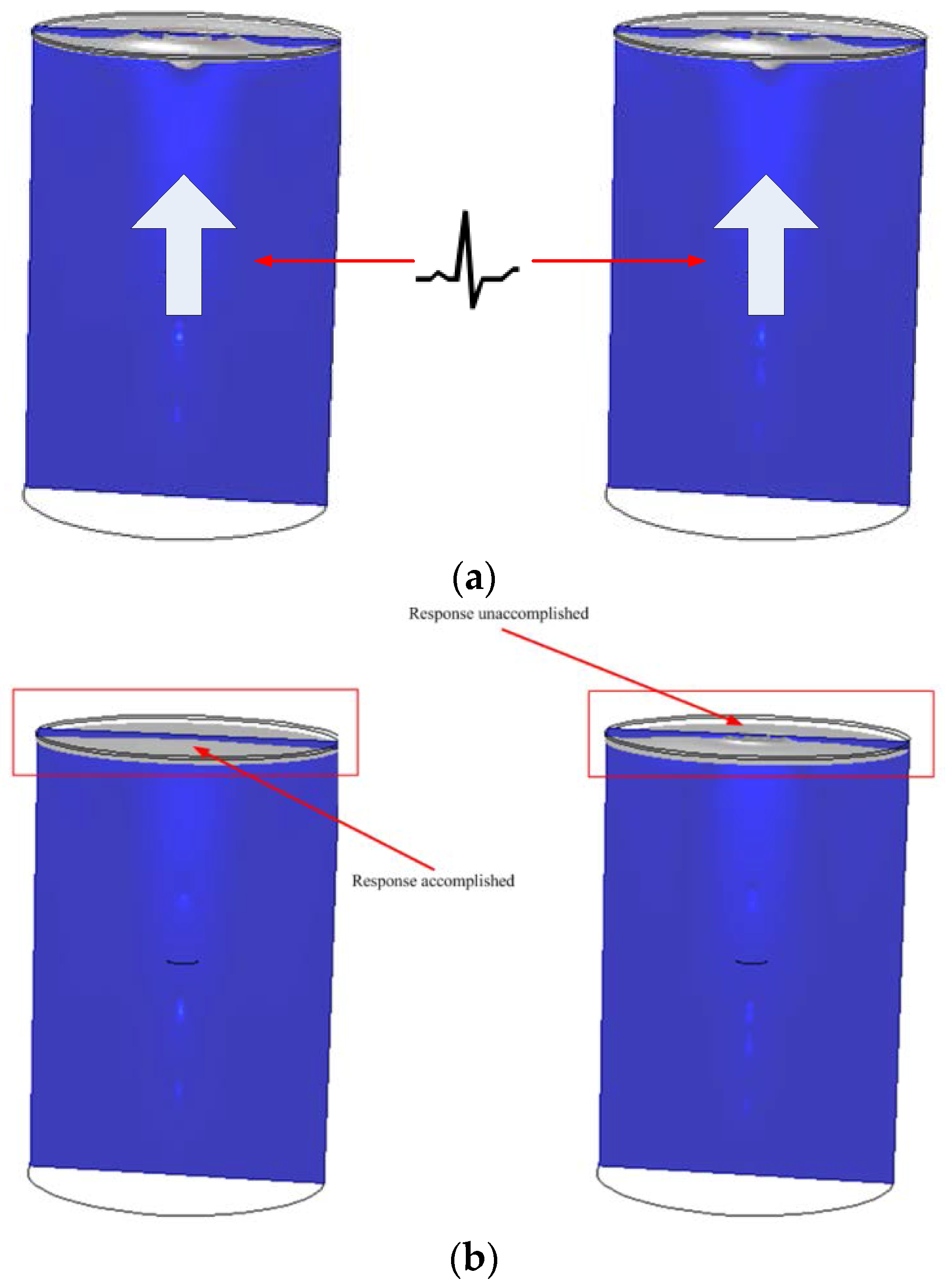
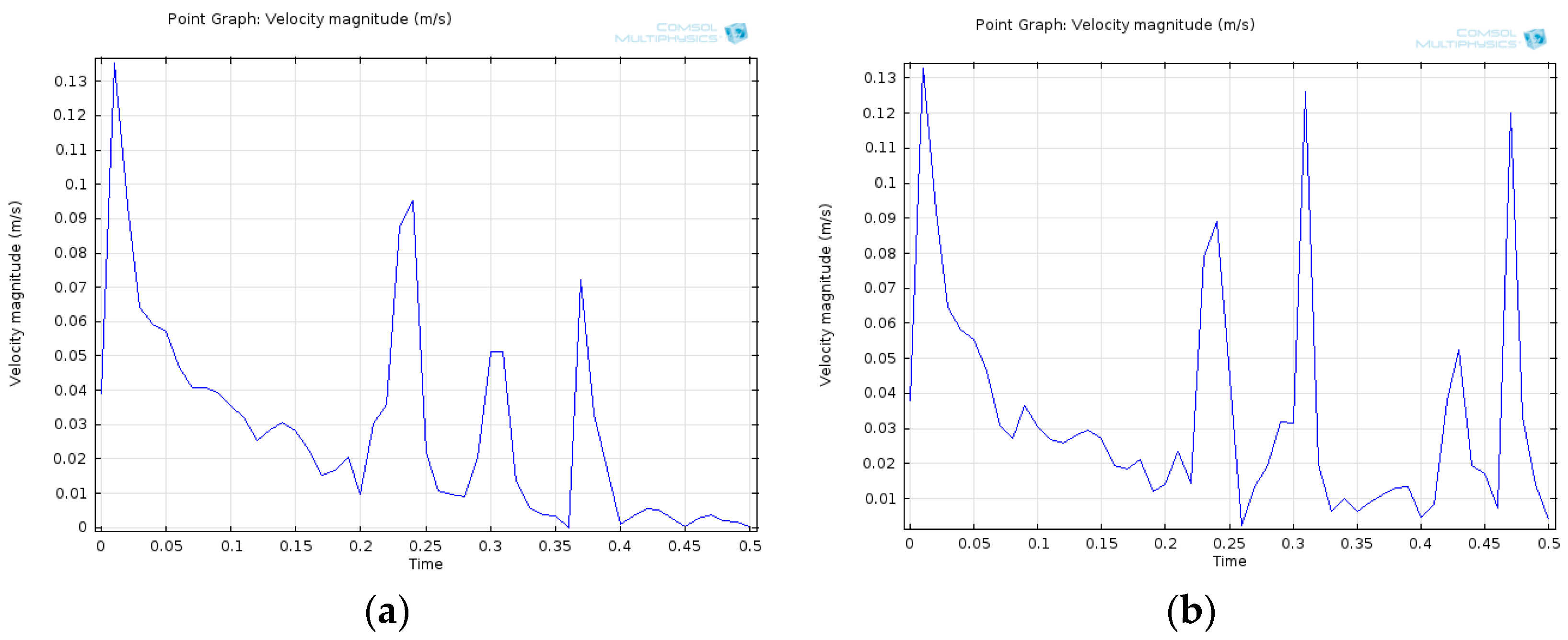
4. Results and Discussion
To support the numerical simulation results, practical experiments comparing different membrane structures were also applied in this paper. The experimental parameters of the materials and the structure and dimensions for membrane are listed in
Table 2.
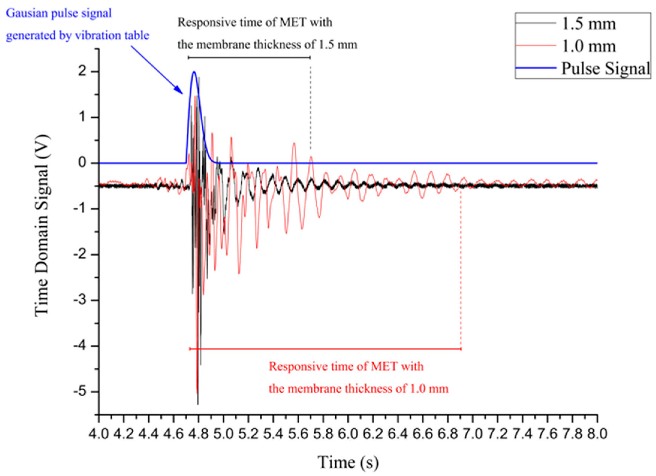
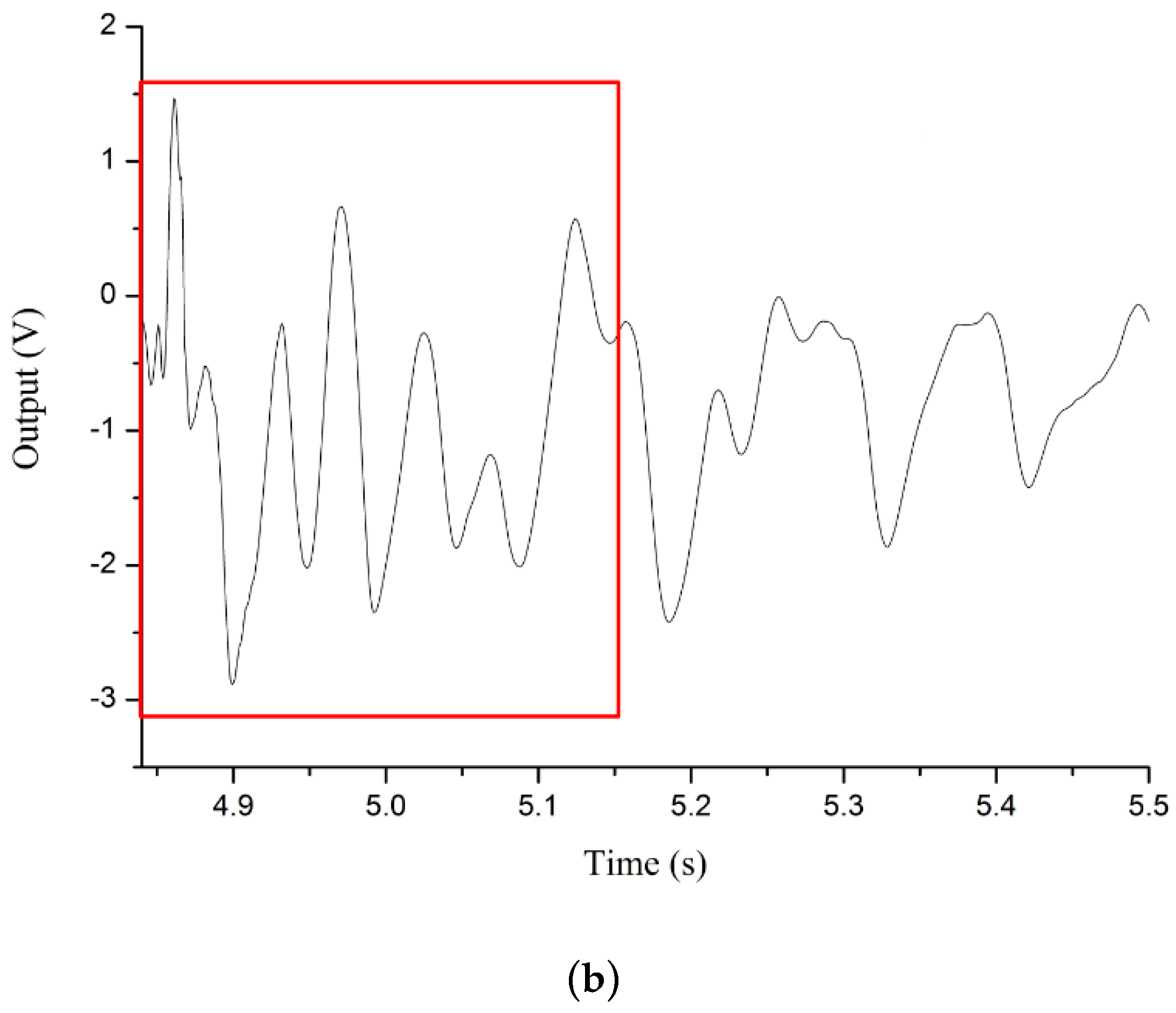
Figure 7 shows the experimental setup and the recorded signals.
By using the NI PXI data acquisition equipment the results of the practical experiment for two METs with different membrane thicknesses are presented in
Figure 8.
By analysing the results shown in
Figure 8, at the beginning, the Gaussian pulse signals marked in blue produce an effective external vibration excitation with the same amplitude for both METs. The MET with the 1.0 mm membrane a longer response time. The MET with a 1.5 mm membrane can regress to the stable state in a shorter time.
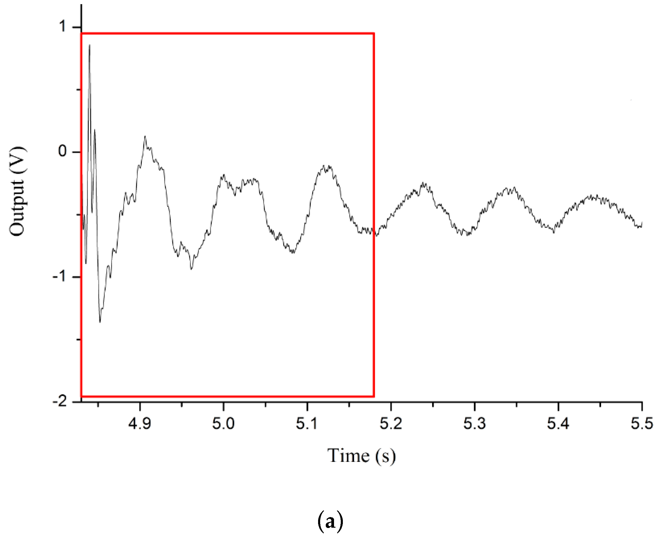
To discuss the correspondence between modelling and the experimental data, a segment captured from the simulation results in
Figure 6 is compared with the experimental result in
Figure 9. First, comparing both the left figures in
Figure 6 and
Figure 9, the MET with the 1.5 mm membrane is activated by an external pulse signal, and the first peak appears in both left figures simultaneously. The peaks following this highest peak dampen gradually, and the curves in the practical experiment convey the same trend. The curves of the right figures in both
Figure 6 and
Figure 9 share the same trend and shape. Therefore, this practical experiment consisting of a pulse signal response test conveys that the results meet the expectations of the numerical simulation in
Figure 6, and the result of the practical experiment in
Figure 9 is presented to verify the numerical simulation.
However, for the dynamic response characteristics, the pulse signal is insufficient to completely reveal the dynamic response characteristics of the MET with different types of membranes. Another practical experiment was studied to investigate the influence of different elastic membranes.
The sensitivity-frequency curves for two types of MET equipped with both membranes are shown in
Figure 10. From the distribution of the points, the dynamic response for the MET can be represented by the result of the practical experiments. In
Figure 10, the MET with the 1.5 mm thick membrane has a higher natural frequency. The natural frequency as a significant parameter affects the sensitivity in the low frequency domain. For a MET that has a low natural frequency, the capacity to detect the low-frequency signal will be much better. The MET with a 1.0 mm thick membrane has a lower natural frequency, so this type of membrane is more suitable for a MET that requires better measurement performance in the low frequency range. However, from the bandwidth point of view, the MET with the 1.0 mm membrane covers a shorter range in the frequency domain. Compared with the 1.5 mm membrane, the MET with the 1.0 membrane always has a narrow band range but a stronger capacity to measure low frequency signals. From the practical experiment data in
Figure 10, the amplitude-frequency characteristics are revealed to describe the dynamic response of the MET.
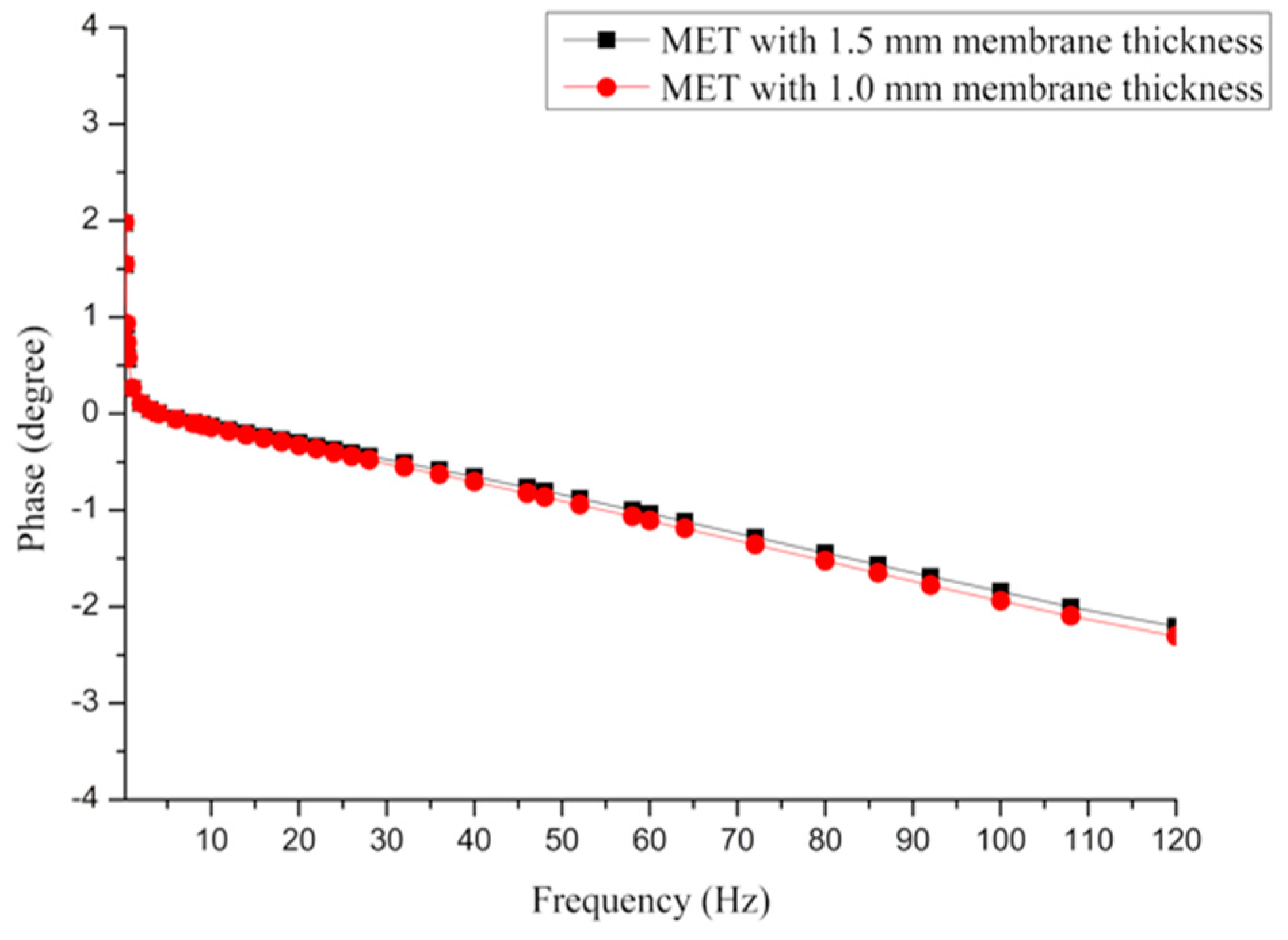
Moreover, to completely study the dynamic response of the MET affected by different types of membranes, another practical experiment involving the phase-frequency characteristics is necessary, and the results are shown in
Figure 11. By comparing two curves from the aspect of phase-frequency, the MET with the 1.5 mm membrane can maintain a little phase shift in the frequency domain. Thus, analysis of the dynamic response for the METs with two types of membrane is explained, and the influence of the elastic membrane is also presented above.


