Remote Evaluation of Rotational Velocity Using a Quadrant Photo-Detector and a DSC Algorithm

Abstract

This paper presents an approach to remotely evaluate the rotational velocity of a measured object by using a quadrant photo-detector and a differential subtraction correlation (DSC) algorithm. The rotational velocity of a rotating object is determined by two temporal-delay numbers at the minima of two DSCs that are derived from the four output signals of the quadrant photo-detector, and the sign of the calculated rotational velocity directly represents the rotational direction. The DSC algorithm does not require any multiplication operations. Experimental calculations were performed to confirm the proposed evaluation method. The calculated rotational velocity, including its amplitude and direction, showed good agreement with the given one, which had an amplitude error of ~0.3%, and had over 1100 times the efficiency of the traditional cross-correlation method in the case of data number N > 4800. The confirmations have shown that the remote evaluation of rotational velocity can be done without any circular division disk, and that it has much fewer error sources, making it simple, accurate and effective for remotely evaluating rotational velocity.

1. Introduction

Rotational parameters, which include angular displacement, velocity and acceleration, can describe the performance, operation states and kinetic characteristics of rotating systems [1,2], such as the vortices of fluid substances, gear transfer systems, rotational machines and fan blades, etc. The exact measurement of transient velocity is vitally important for accurately controlling and monitoring the movements of some bodies, and for acquiring fault information in machine diagnoses [3]. Thus the method of sensing rotational velocity can be used for the analyses, monitoring and control of mechanical systems, swirling gas- or fluid flow, etc.

For sensing rotational or angular velocity, there exist methods using gyroscopes, marking methods, interferometry, correlation methods, circular grating sensing and spatial filtering methods, etc. The gyroscope method using a Sagnac-effect-based integrated gyroscope with small footprint has high resolution, and can sense transient angular velocity [4,5,6]. However it is not suitable for remote measurement and super-low velocity, and can be affected by environmental factors [7,8]. The interferometry methods, including Fabry-Perot cavities and Mach-Zehnder interferometers, have complicated structures and high precision fabrication requirements [9,10,11]. In the correlation method, the traditional cross-correlation (TCC) is often used to process the output signals of two identical sensors in the measured region [12,13,14], which provides non-contact measurements with low cost for monitoring gas-solid and solid-liquid flows [15,16,17,18]. The image matching method, in which a high-speed camera captures a series of instantaneous images to calculate velocity, also belongs to the correlation methods [19,20,21,22]. Correlation methods are less applied for remotely sensing transient angular velocity, due to the numerous multiplication operations required. Marking methods with optical labels (plus quadrant photodiode) or Hall-effect sensors mainly sense average rotational velocities with lower resolution or direction ambiguity [23,24], which can hardly measure instantaneous rotational velocity. The methods based on circular gratings like optical gratings [25,26] and magnetic grids can be employed to sense the transient angular velocity of target objects with high resolution [27,28]. Their circular gratings must be set up as circular division disks to be coaxially mounted on the measured object, and their resolution and precision are dependant on the grating grooves. Optical gratings are easily destroyed by tiny dust particles and greasy dirt. In some cases such as those of high-speed rotating machines or when measuring gas- or fluid flows, etc., circular benchmarks cannot be mounted on the measured systems die to limitations in their structures, or their performances are possibly deteriorated. In the spatial filtering (SF) method [29], a center coefficient is obtained from the central frequencies of the output signals of two differential spatial filters. Then the rotational velocity is calculated with the central frequencies and the center coefficient, and its direction is determined by the center coefficient and one linear displacement direction. Rotational velocity measurements using the SF method are complicated, since they need to compute all the center coefficients, the central frequencies and the displacement direction.

This paper will present a novel approach for remotely evaluating transient rotational velocities with a quadrant photo-detector (QPD) and a differential subtraction correlation (DSC) algorithm proposed by us, which does not require any circular indexing plates or benchmarks. The QPD outputs four random signals, from which the amplitude and direction of the rotational velocity are obtained simultaneously by using the DSC algorithm that only needs addition and subtraction operations without any multiplication or division, which should make it faster than other correlation methods. This paper is organized as follows: Section 2 shows the rotational velocity sensing system; Section 3 describes its evaluation principle in detail; Section 4 presents some experimental calculations to verify the proposed approach, and the final section gives our conclusions.

2. System for Sensing Rotational Velocity

The quadrant photo-detector for sensing rotational- or angular-velocity, shown in Figure 1, is formed by four photovoltaic cells PD1, PD2, PD3 and PD4. PD1 and PD2 are arranged in parallel each other with distance P, which constitute a linear velocity sensor (LVS1), and output signals S₁ and S₂.

Similarly, PD3 and PD4 are also arranged in parallel each other with the distance P, which lead to another linear velocity sensor (LVS2), and output signals S₃ and S₄. The LVS1 and LVS2 are also aligned in parallel each other at the interval of L, and then form the QPD.

The rotational velocity sensing system with the QPD and the DSC algorithm is schematically illustrated in Figure 2. Suppose the terminal plane of a measured object has a rough surface, and rotates around center O’ with a rotational velocity ω. The surface of the terminal plane is imaged on the QPD through an optical telescope system with magnification M. The image of the measured object rotates around center O that is the imaged point of center O’, and it must cover the QPD. Thus the size of the terminal plane must be at least larger than L/M. The distances of center O to LVS1 and LVS2 are R₁ and R₂, respectively. The output signals of the QPD are random, owing to the stochastic reflection image of the terminal plane. The output signals S₁, S₂, S₃ and S₄ will go to the data processing system (DPS) after they are amplified and converted into digital signals. In the DPS, the DSC between S₁ and S₂ is calculated and noted as DSC1, which is related to the linear velocity of moving image on PD1 and PD2. The DSC between S₃ and S₄ is also obtained and denoted as DSC2, which indicates the linear velocity of moving image on PD3 and PD4. The rotational velocity ω of the measured object can be derived from the DSC1 and DSC2.

3. Principle of Evaluating Rotational Velocity with DSC

3.1. Image Velocity on QPD

Supposing that the terminal plane of measured object rotates around the O’ in the rotational velocity of ω, the terminal plane and its imaged plane are depicted in Figure 3a,b, respectively, which are viewed from the optical telescope system. LVS1’, LVS2’ and O’ on the terminal plane are conjugated to LVS1, LVS2 and O on the image plane, respectively.

In Figure 3a, D’₁ and D’₂ are two arbitrary points on the central line of the LVS1’. The interval between O’ and the central line of LVS1’ is R’₁, and the distances of O’ to D’₁ and D’₂ are R’_D1 and R’_D2, respectively. In Figure 3b, D₁ and D₂ are the conjugate points of D’₁ and D’₂, respectively, thus the distances of O to D₁ and D₂ are R_D1 = MR’_D1 and R_D2 = MR’_D2, respectively. With the rotational velocity of ω, the linear velocities at D₁ and D₂ are V_D1 = ωMR’_D1 = ωR_D1 and V_D2 = ωMR’_D2 = ωR_D2, respectively. V_D1 and V_D2 have the components V_D1 × cosα and V_D2 × cosβ, respectively, in the direction of LVS1, where α and β are the angles of R₁ relative to lines OD₁ and OD₂, respectively.

Meanwhile, R_D1 × cosα = R_D2 × cosβ = R₁, thus the image velocity V₁ on any point of the central line of the LVS1 can be obtained, such that:

$$V_1=\mathsf{\omega }{R}_1$$

(1)

Similarly, we can also get the image velocity V₂ on any point of the central line of the LVS2, governed by:

$$V_2=\mathsf{\omega }{R}_2$$

(2)

where R₂ is the interval between O and the central line of LVS2. The image velocities V₁ and V₂ are insensitive to the variation of the amplification coefficient M which has been hidden in R₁ and R₂ on the image plane.

3.2. Characteristics of Output Signals of QPD

When a light source illuminates the terminal plane of the measured object that has a rough surface with finite and stochastic reflection, some light rays will be scattered by the rough surface, and then be imaged on the QPD through the optical telescope system with a high cut-off frequency in the spatial domain. The image on the QPD locating the image plane is randomly distributed, and has a wide spatial bandwidth. The output signal of each photovoltaic cell in the QPD is the integration of the randomly-reflected light intensity on its active area, which is also stochastic. Thus the QPD outputs four stochastic signals that are related to the random distribution of the rotating image, and the relations among the QPD output signals are involved with the image movement decided by the rotation of the terminal plane.

It is assumed that the central lines of LVS1 and LVS2 are x-axes that are parallel with PD1–PD2 and PD3–PD4, respectively. Figure 4 shows schematically the stochastic light-intensity distributions on the active areas of the QPD whose PD1–PD4 positions are also indicated in x-y coordinate, where f₁(x) and f₂(x) are the examples of actual light-intensity distributions along the LVS1 and the LVS2, respectively, x₀ is the x-axial position of PD1 and PD3, c is the width of the photovoltaic cells.

If only considering x-axial movement, the integration of the y-axially distributed random light at x-position can be taken as the whole light intensity at x-position, which ignores the y-axial factor and still is a stochastic distribution on the x-axis, shown as f₁(x) or f₂(x). When the rough surface of a measured body is imaged on the QPD, the QPD will be illuminated by the randomly distributed light that is regarded as only an x-axial distribution, and the output signals of the PD1–PD4 are the integrations of the light intensity distributions f₁(x) or f₂(x) in the x-axial widths of the PD1–PD4, respectively. If the measured body is rotating, its scattering light will be randomly changed, and then the QPD will output signals S₁, S₂, S₃ and S₄ that are stochastic in time domain.

If the LVS1 (PD1) is at position x₀, its output signals S₁ and S₂ will be the integrations of f₁(x) in the regions of PD1 and PD2, respectively, and they have the relation S₂(x₀) = S₁(x₀ − P). If the image on the LVS1 is moving in the image velocity V₁, then the space-time relation x₀ = V₁t allows S₁(x₀) and S₂(x₀) to become time-domain signals S₁(t) and S₂(t), described by:

$$\begin{array}{l}{S}_1(t)={\displaystyle {\int }_{x_0/V_1}^{(x_0+c)/V_1}{f}_1(V_{1}t)V_{1}dt}\\ S_2(t)={\displaystyle {\int }_{(x_0+P)/V_1}^{(x_0+P+c)/V_1}{f}_1(V_{1}t)V_{1}dt}\end{array}\}$$

(3)

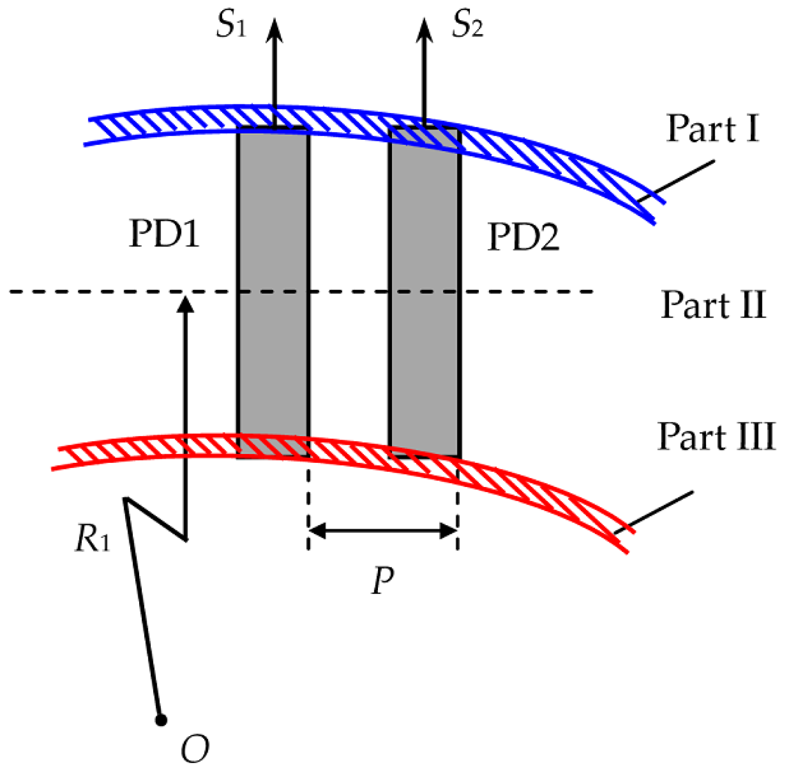
The active-area factor of the photovoltaic cells cannot be ignored, thus the integrations in S₁(t) and S₂(t) will filter some high-frequency components of the light intensity distributions on PD1 and PD2, which actually function as low-pass filters that can remove much relevant characteristic information. When the measured object revolves around O’, its image on PD1 and PD2 can be divided into three parts: I, II and III, as illustrated in Figure 5.

Part I and Part III are labeled by blue slanted lines and red slanted lines, respectively, and Part II is the region between Part I and Part III. Part II with the largest area makes principal contribution to S₁(t) and S₂(t), and Parts I and III can be ignored because of their much less contributions. On other hand, the image of Part II on PD1 will be on PD2 after the delay time τ₁ = P/V₁. Thus Equation (3) indicates that S₂(t) is approximately equal to the temporally delayed signal of S₁(t) with the delay time of τ₁, which can be written as:

$$S_2(t)\approx S_1(t-{\mathsf{\tau }}_1)$$

(4)

where τ₁ > 0 represents the movement direction from left to right, and τ₁ < 0 represents that from right to left. Once τ₁ is ascertained, the image velocity V₁ on the LVS1 will be determined by:

$$V_1=\mathsf{\omega }{R}_1=P/{\mathsf{\tau }}_1$$

(5)

Like the analogous S₁(t) and S₂(t), S₄(t) is also approximately equal to the temporally delayed signal of S₃(t) with the delay time of τ₂, which is expressed to be S₄(t) ≈ S₃(t − τ₂) where τ₂ = P/V₂ is the time delay of S₃(t). τ₂ > 0 also indicates the movement direction from left to right, and τ₂ < 0 indicates that from right to left. Once τ₂ is obtained, the image velocity V₂ on the LVS2 will be also calculated with:

$$V_2=\mathsf{\omega }{R}_2=P/{\mathsf{\tau }}_2$$

(6)

Based on the above descriptions, we can establish the features of the temporal output signals of the QPD: (1) they are random, corresponding to the spatially-stochastic reflection of the terminal plane; (2) the signals S₂(t) and S₄(t) are approximately interrelated to S₁(t) and S₃(t), respectively; (3) some high-frequency information consisting of more useful characteristics has been filtered, which is a disadvantage to correlation analysis. If the delay times τ₁ and τ₂ are obtained, Equations (5) and (6) may let the rotational velocity ω be calculated. According to the abovementioned features, the DSC algorithm is exploited to derive the delay times from the output signals.

3.3. Differential Subtraction Correlation

The output signals of the QPD are random and correlative, thus we also employ correlation analysis to calculate τ₁ and τ₂. However the conventional correlation method is low efficient, due to its multiplication operations with the complexity of about O(3Nlog₂N) or O(N²), where N is the number of sampling data. In order to fast and exactly determine the delayed time, we propose the DSC to analyze the correlation ϕ₁(τ) between S₁(t) and S₂(t), defined as:

$${\mathsf{\phi }}_1(\mathsf{\tau })={\displaystyle \underset{T_1}{\overset{T_2}{\int }}\left|\frac{d{S}_1(t-\mathsf{\tau })}{dt}-\frac{d{S}_2(t)}{dt}\right|}dt={\displaystyle \underset{T1}{\overset{T_2}{\int }}\left|d{S}_1(t-\mathsf{\tau })-d{S}_2(t)\right|}$$

(7)

where T₁ and T₂ are the start time and end time, respectively, of the integration. In practice, S₁(t) and S₂(t) are converted into digital signals s₁(n) and s₂(n), respectively, by using a multi-channel A/D converter with sampling interval T₀. Thus the DSC ϕ₁(τ) is discretized into Φ₁(m) (i.e., DSC1) as:

$${\mathsf{\Phi }}_1(m)={\displaystyle \sum _{n=N_1}^{N_2-1}\left|s_1(n-m+1)-s_1(n-m)-s_2(n+1)+s_2(n)\right|}$$

(8)

where N₁ = T₁/T₀, N₂ =T₂/T₀ and m = τ/T₀ are integral. If S₂(t) = S₁(t − τ₁), Φ₁(m) will go to zero at m = m₁ = τ₁/T₀, and is much more than 0 at other m, where m₁ is an integer representing the temporal delay τ₁.

Similarly, the output signals S₃(t) and S₄(t) of the LVS2 are converted into digital signals s₃(n) and s₄(n), respectively, with the same sampling interval T₀. Then s₃(n) and s₄(n) are sent to the DPS to calculate the discrete DSC Φ₂(m) (i.e., DSC2) between s₃(n) and s₄(n), given by:

$${\mathsf{\Phi }}_2(m)={\displaystyle \sum _{n=N_1}^{N_2-1}\left|s_3(n-m+1)-s_3(n-m)-s_4(n+1)+s_4(n)\right|}$$

(9)

If S₄(t) = S₃(t − τ₂), Φ₂(m) will also go to zero at m = m₂ = τ₂/T₀, and is much more than 0 at other m, where m₂ is an integer representing the temporal delay τ₂.

In practice, the output signals of the QPD in this rotational velocity sensing system have the relations S₂(t) ≈ S₁(t − τ₁) and S₄(t) ≈ S₃(t − τ₂), which let Φ₁(m) and Φ₂(m) go to the minimums at m = m₁ and m = m₂, respectively, and they are much more than 0 at other m. Based on Equations (8) and (9), the DSC algorithm is then described as follows:

(1) Acquiring s₁(n), s₂(n), s₃(n) and s₄(n) by discretizing the output signals of the QPD with synchronous four-channel A/D converter;

(2) Calculating the DSC1 and DSC2 at different m, according to Equations (8) and (9) with s₁(n), s₂(n), s₃(n) and s₄(n);

(3) Searching the minimums of Φ₁(m) and Φ₂(m), and taking the serial numbers at the minimums of Φ₁(m) and Φ₂(m) as the temporal-delay numbers m₁ and m₂, respectively.

The temporal-delay numbers m₁ and m₂ have indicated the delay times τ₁ and τ₂, respectively. The proposed DSC algorithm just requires subtraction, absolute and addition operations without any multiplications or divisions, so it can facilitate the fast correlation calculation of two random signals. Furthermore, its difference operation between two adjacent data can recover high-frequency components, and can eliminate low-frequency noise and shift, and then can enlarge the differences between adjacent data, which are advantageous to improve accuracy.

3.4. Evaluation of Rotational Velocity

According to the DSC algorithm described before, m₁ and m₂ can be derived from Φ₁(m) and Φ₂(m) by searching the minima of Φ₁(m) and Φ₂(m), respectively. Because τ₁ = m₁T₀ and τ₂ = m₂T₀, m₁ > 0 and m₂ > 0 indicate the image movement directions from left to right on the LVS1 and the LVS2, respectively, and m₁ < 0 and m₂ < 0 indicate that from right to left on the LVS1 and the LVS2, respectively. Thus Equations (1), (2), (5) and (6) lead to the relations of the rotational velocity ω with m₁ and m₂, governed by:

$$\mathsf{\omega }{R}_1=P/(m_1{T}_0)$$

(10)

$$\mathsf{\omega }{R}_2=P/(m_2{T}_0)$$

(11)

Now let us suppose that the LVS1 is above the LVS2. The location of the rotational center O on the image plane may be between the LVS1 and the LVS2, below both the LVS1 and the LVS2, or above both the LVS1 and the LVS2, as shown in Figure 6a–c, respectively.

The signs of m₁ and m₂ represent the image movement directions on the LVS1 and LVS2, which can be used for judging the rotational center locations and directions. In Figure 6a, the sign of m₁ is always different from that of m₂, and m₁ > 0 and m₁ < 0 demonstrate the clockwise rotational direction and the counter-clockwise one, respectively. In Figure 6b,c, the sign of m₁ is always the same as m₂, and their rotational center locations can be discriminated by comparing m₁ to m₂, where |m₁| < |m₂| and |m₁| > |m₂| as indicated in Figure 6b,c, respectively, owing to the fact R₂ ± L = R₁. In Figure 6b, m₁ > 0 and m₁ < 0 illustrate the clockwise rotational direction and the counter-clockwise one, respectively. In Figure 6c, m₁ < 0 and m₁ > 0 mean the clockwise rotational direction and the counter-clockwise one, respectively. At the same time, Figure 6a–c have shown R₁ + R₂ = L, R₁ − R₂ = L with |m₁| < |m₂|, and R₂ − R₁ = L with |m₁| > |m₂, respectively, from which we can derive the rotational velocity ω as (1/m₁ − 1/m₂)P/(LT₀) by using Equations (10) and (11). The sign of ω is the same as that of m₁ in the cases of Figure 6a,b, and is opposite that of m₁ in the case of Figure 6c, which shows that ω > 0 and ω < 0 always represent the clockwise rotational direction and the counter-clockwise one, respectively. Thus in all cases of different directions and centers, the sign of ω always indicates the rotational direction, and the rotational velocity ω can be determined by:

$$\mathsf{\omega }=\frac{P}{L{T}_0}\left(\frac{1}{m_1}-\frac{1}{m_2}\right)$$

(12)

Note that |m₁| and |m₂| are not equal to 0 in Equation (12), and must be less than N at least in the DSCs. In practice, they should be less than N/2, in order to accurately acquire them. Thus the better range of the rotational velocity calculated with Equation (12) should be from 2P/(NT₀R_min) to P/(T₀R_max), where R_min = min(R₁, R₂) and R_max = max(R₁, R₂).

The relations of ω with m₁, m₂, rotational center location and direction are listed in

Table 1. The relations of ω with rotational direction, center location, m₁ and m₂.

Rotational Direction	Relation of m1 with m2	Judgment Results
		Location of the Rotational Center O	Sign of ω
Clockwise	m1 > 0, m2 < 0	Between LVS1 and LVS2	+
	0 < m1 < m2	Below both LVS1 and LVS2	+
	m1 < m2 < 0	Above both LVS1 and LVS2	+
Counter-clockwise	m1 < 0, m2 > 0	Between LVS1 and LVS2	−
	0 > m1 > m2	Below both LVS1 and LVS2	−
	m1 > m2 > 0	Above both LVS1 and LVS2	−

. The rotational velocity ω calculated with Equation (12) includes the amplitude and direction of the rotational velocity on the image plane, which is corresponding to the rotational velocity of the measured object. Therefore once m₁ and m₂ are obtained, the rotational velocity consisting of its amplitude and direction will be calculated by only using Equation (12).

4. Experimental Calculations

The rotation of a planar wooden disk with rough surface is taken as an example to confirm the validity of the proposed method for remotely sensing rotational velocity. The confirmation can be realized according to the following steps: (1) The wooden disk is installed on the shaft of a DC-micromotor (Model 2230G0003, Faulhaber GmbH & Co. KG, Schönaich, Germany) which drives the rotation of the disk. The angular speed of the DC-micromotor is controlled by the output voltage of an adjustable DC regulated power supply (Model APS3005S-3D, Atten Technology Co., Shenzhen, China); (2) The rotational velocity of the wooden disk is set by adjusting the output voltage and then measuring the rotational velocity with a DT-2234B Digital Tachometer (Suwei Co. Ltd., Guangzhou, China); (3) Sunlight or very bright white LEDs illuminate the wooden disk whose surface is imaged on a QPD through a telecentric imaging system (telescope) with magnification of 1×. The telecentric imaging system includes an adjustable aperture and two composite objectives with a focal length of ~26 mm. The QPD is constructed by four identical photovoltaic-cells with the active area of 0.89 × 4.39 mm², where two photovoltaic cells of each linear velocity sensor (LVS1/LVS2) directly come from two adjacent pixels of a Si-based photovoltaic-cell array (Model A5V-38, OSI Optoelectronics Inc., Hawthorne, CA, USA), and then the LVS1 and LVS2 form the QPD. Other parameters of the QPD are as follows: P = 0.99 mm and L = 16 mm; (4) The output signals of the QPD are amplified and then converted into discrete data by four A/D converters with the sampling interval of T₀ = 0.2 ms. The amplifier and the A/D converter are INA128 (Texas Instruments Inc., Dallas, TX, USA) and AD7663 (Analog Devices Inc., Norwood, MA, USA) with 16-bit resolution, respectively; (5) The discrete data are sent to a DPS, in which Φ₁(m) and Φ₂(m) are calculated, and their minimums are searched to get m₁ and m₂. Then the rotational velocity ω is calculated with Equation (12); (6) Finally, we compare the calculated value and direction to the given ones, and judge whether they are agree with each other.

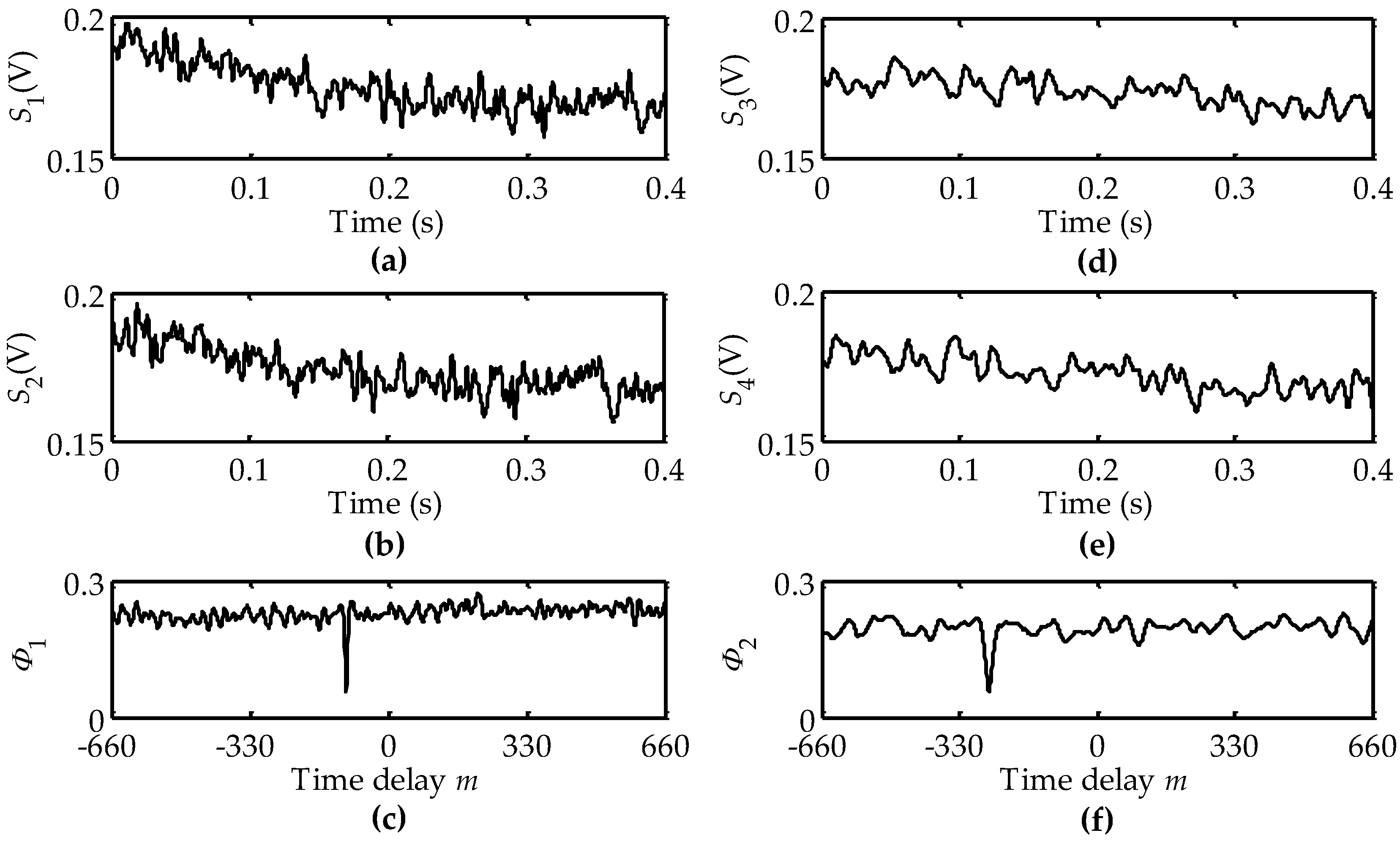
When the wooden disk was rotated at a rotational velocity of 6.3 rad/s in the clockwise direction, we located the rotational center O, whose distance to its closest LVS was ~6 mm, to be between the LVS1 and the LVS2. The output signals S₁(t), S₂(t), S₃(t) and S₄(t) of the QPD are shown in Figure 7a,b,d,e, respectively. Figure 7c,f illustrate the calculated Φ₁(m) and Φ₂(m), respectively. The minima of Φ₁(m) and Φ₂(m) were searched at m₁ = 79 and m₂ = −131, respectively. According to Equation (12), the calculated rotational velocity was 6.278 rad/s with the “+” sign that represents the clockwise direction. These results demonstrate that the calculated value and direction of the rotational velocity agree with the given ones.

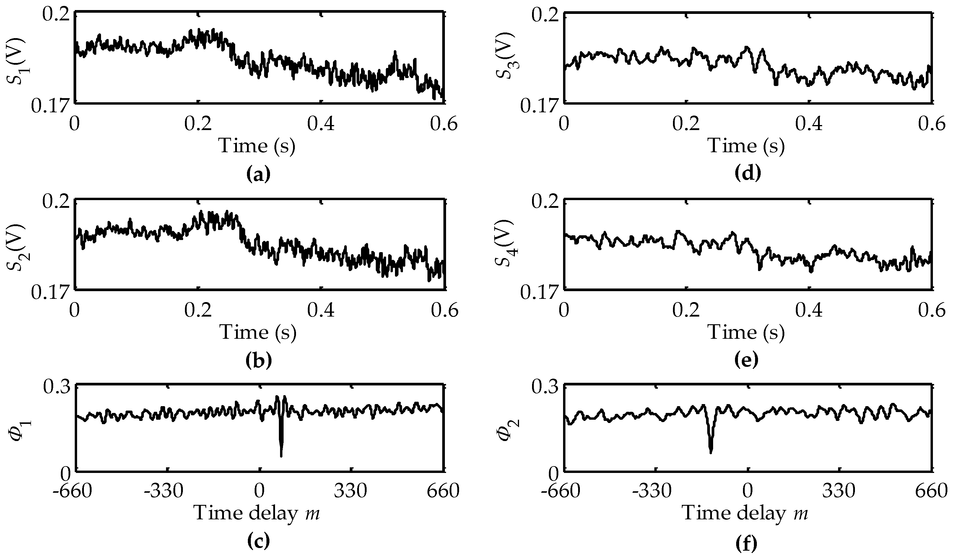
When the wooden disk rotated counter-clockwise at a rotational velocity of 1.9 rad/s, we let the rotational center O, whose interval to its nearest LVS was ~10 mm, be below both the LVS1 and the LVS2. The output signals S₁(t), S₂(t), S₃(t) and S₄(t) are exhibited in Figure 8a,b,d,e, respectively. Figure 8c,f plot the calculated DSCs Φ₁(m) and Φ₂(m), respectively, from which we derived m₁ = −100 and m₂ = −260. Based on Equation (12), the calculated rotational velocity was −1.904 rad/s whose “−” sign indicates the counter-clockwise direction. The calculated rotational velocity including its amplitude and direction is also in agreement with the given one. Similarly, we performed the corresponding experimental calculations in the cases of other rotational directions and center locations, where the calculated rotational velocities were also in agreement with their given ones.

The abovementioned calculations had a relative amplitude error of ~0.3%. Their resolutions were up to 0.011 rad/s, and their optimal resolution was 5.4 × 10⁻⁵ rad/s (N = 4800). The resolution and its optimum of the DSC-based rotational velocity are actually determined by P/(LT₀m₁m₂) and 4P/(LT₀N²), respectively, which are related to the sampling interval T₀ and the rotational velocity. For measuring super-low rotational velocities, the resolution can be improved to be excellent by increasing the sampling interval in the case of guaranteeing enough precision. In other often used methods, the resolution of laser gyroscopes can reach 0.01°/h~10°/h [4], and the TCC-based method has a relative error of 3.33% [12]. The marking method with an optical label plus quadrant photodiode possesses a relative error of 0.001% [24], while it measures only the average rotational velocity within the angular displacement of 2π rad. The circular-grating-based methods with Moiré optical grating and capacitive grating have relative errors of ~0.07% and 0.44%, respectively [30]. Compared to the existing method, the DSC-based method proposed has mid-ranking resolution and accuracy, whereas on the plus side, it does not require installing any standard division disk.

To verify the computational speed, the DSC-based and TCC-based calculations were performed in an Acer PC system equipped with an Intel dual-core i3-processer plus 3.4 GHz, OS Windows 10 and Matlab 2010. The DSC-based calculations needed average times of 141 ms and 86 ms in the cases of N = 4800 and N = 3600 data numbers, respectively, and the TCC-based ones consumed on average times of 158.92 s and 72.849 s, correspondingly. These achievements imply that the DSC-based computational speed has been improved up to 1127 times that of the TCC-based one in the case of a data number N > 4800. Thus the DSC-based calculation for rotational velocity is very fast and accurate, and is not affected by the movement and alignment error of the QPD relative to the measured object, making it fit for remotely evaluating transient angular-velocities. These features are due to the following reasons: (1) (1/m₁ − 1/m₂) always makes |R₁ ± R₂| equal to constant L, in the cases of arbitrary rotational center, eccentricity, radial fluctuation or parallel movement; (2) the amplification coefficient M has been hidden in R₁ and R₂ on the image plane, which leads to the insensitivity to various M changed by alignment error and axial shaking; (3) V₁ ± V₂ is always not related to eccentricity, parallel movement and radial shift. Thus the rotational velocity calculated with Equation (12) is only determined by pure rotation, which has much fewer error sources.

5. Conclusions

The method of remotely evaluating rotational velocity has been presented in this paper, where the rotational velocity is derived from the temporally-delayed serial-numbers at the minima of two DSCs that are calculated with the four stochastic output signals of the QPD formed by four identical photovoltaic-cells, and the sign of the rotational velocity represents the rotational direction. The DSC algorithm is implemented by differentiating and subtracting the random output signals of two photovoltaic cells, and then integrating the absolute value of the differential subtraction signal. In the DSC algorithm, the rough surface and random reflection of measured object will have a contribution to precisely determining the temporal delay and rotational velocity, owing to its difference operation. Experimental calculations were performed to confirm the proposed evaluation method. The calculated rotational velocities, including their amplitudes and directions, were in excellent agreement with their given ones, which possessed an amplitude error of ~0.3%, and had over 1100 times the TCC-based efficiency in the case of data number N > 4800.

The proposed evaluation method works without any circular indexing plate, and its DSC does not require any multiplication or division operations. At the same time, this method is insensitive to the radial fluctuation, axial shift, eccentricity and parallel movement of the measured object that has assembly or mismatch errors. The rotational velocity calculated with Equation (12) is only determined by pure rotation, which has many fewer error sources. Comparing to the SF method, this evaluation method does not require calculating central frequencies, center position and extra direction, and it can simultaneously determine the amplitude and direction of a measured rotational velocity. In general, the proposed method is simple, fast, accurate and effective for remotely evaluating transient rotational velocities.