
Improvement of Depth Profiling into Biotissues Using Micro Electrical Impedance Spectroscopy on a Needle with Selective Passivation

Abstract
:1. Introduction
2. Materials and Methods
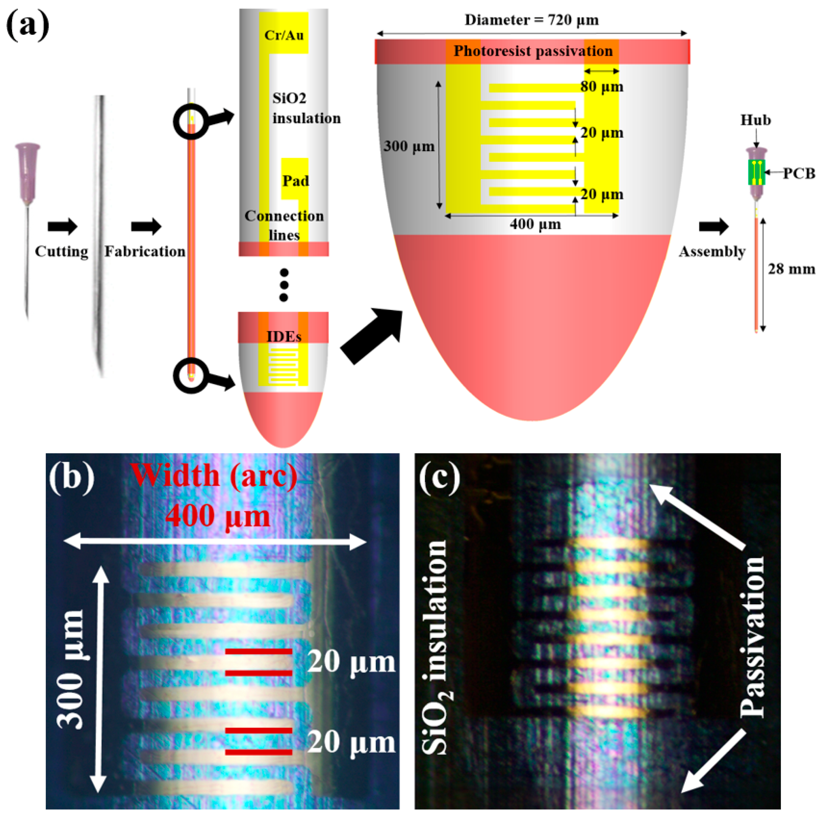
2.1. Device Design
2.2. Device Fabrication
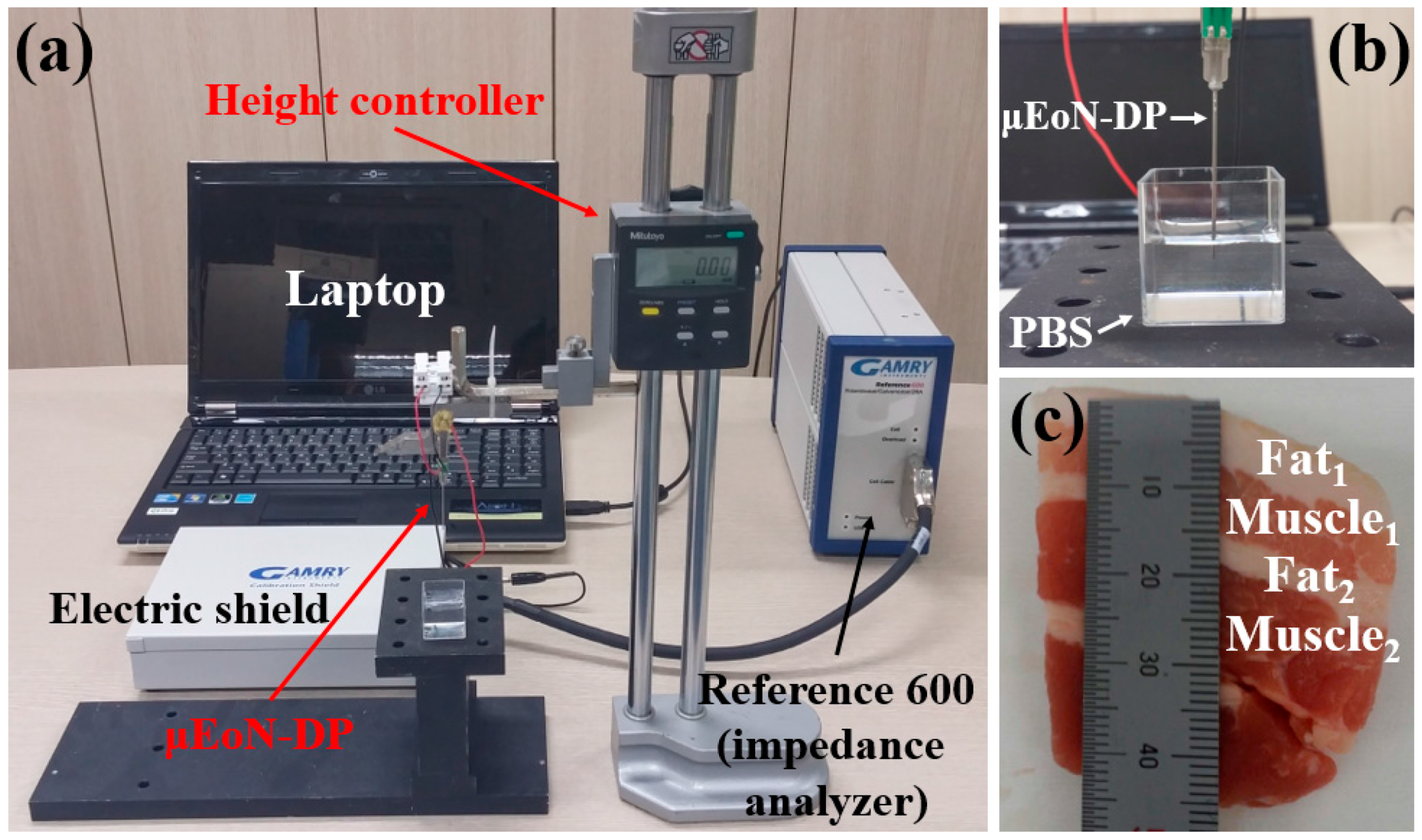
2.3. Experimental Setup
3. Results and Discussion
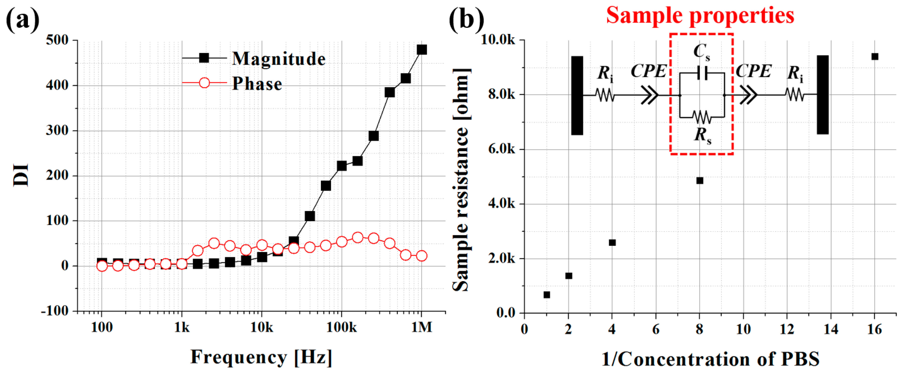
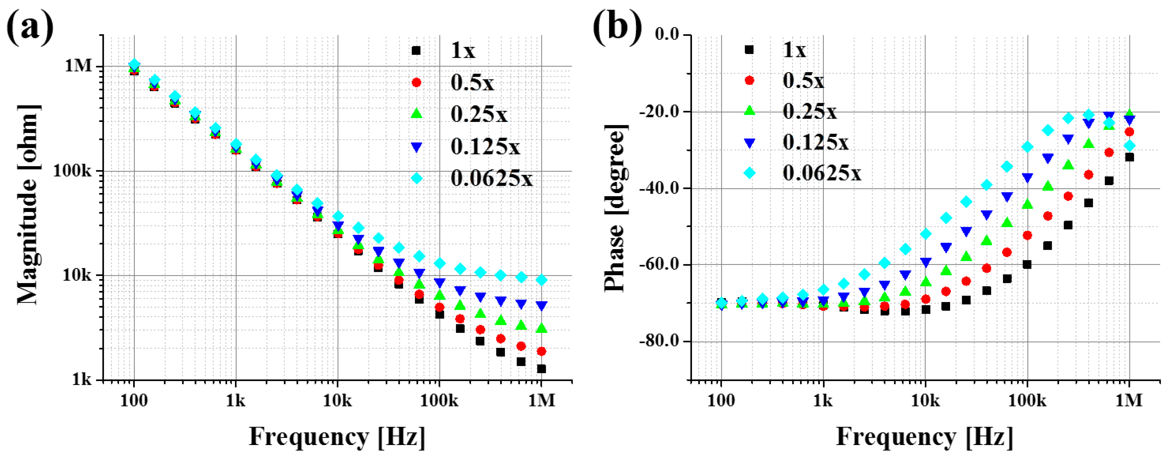
3.1. PBS at Various Concentration Levels
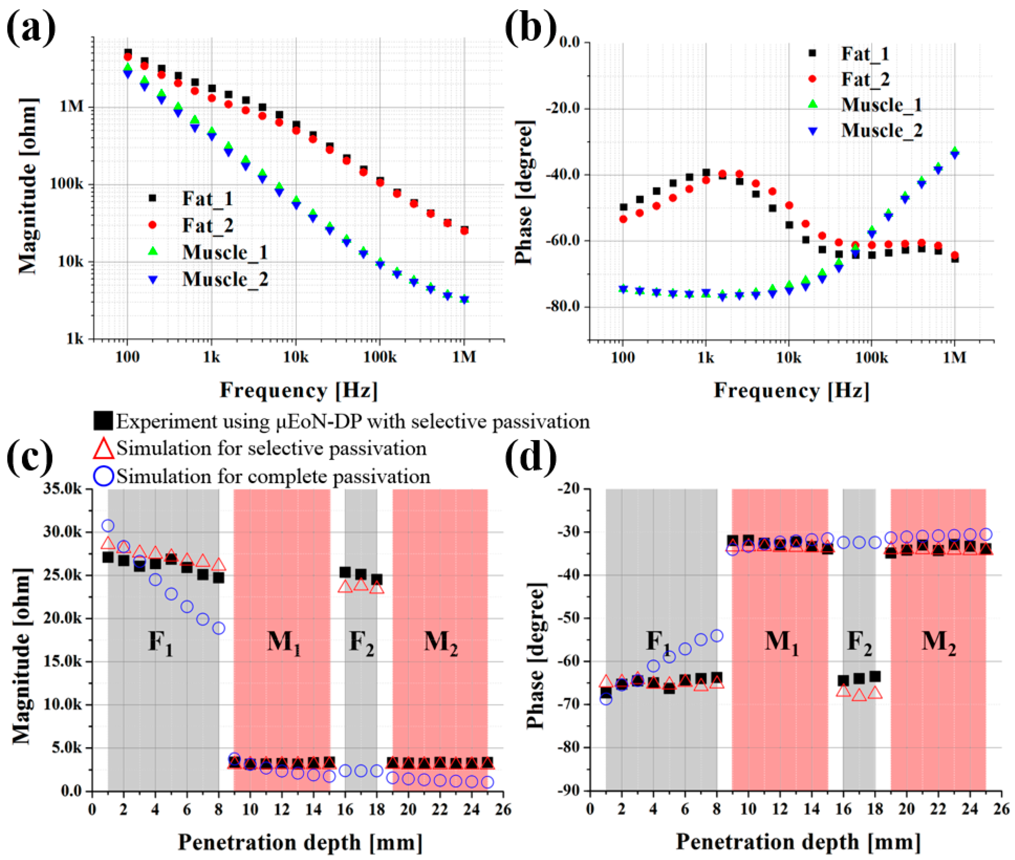
3.2. Depth Profiling Into Four-Layered Porcine Tissue
3.3. Simulation Verification of Selective Passivation Layer
4. Conclusions
Acknowledgments
Author Contributions
Conflicts of Interest
References
- Babahosseini, H.; Srinivasaraghavan, V.; Zhao, Z.; Gillam, F.; Childress, E.; Strobl, J.S.; Santos, W.L.; Zhang, C.; Agah, M. The impact of sphingosine kinase inhibitor-loaded nanoparticles on bioelectrical and biomechanical properties of cancer cells. Lab Chip 2016, 16, 188–198. [Google Scholar] [CrossRef] [PubMed]
- Kang, G.; Kim, Y.-J.; Moon, H.-S.; Lee, J.-W.; Yoo, T.-K.; Park, K.; Lee, J.-H. Discrimination between the human prostate normal cell and cancer cell by using a novel electrical impedance spectroscopy controlling the cross-sectional area of a microfluidic channel. Biomicrofluidics 2013, 7, 044126. [Google Scholar] [CrossRef] [PubMed]
- Kurz, C.M.; Büth, H.; Sossalla, A.; Vermeersch, V.; Toncheva, V.; Dubruel, P.; Schacht, E.; Thielecke, H. Chip-based impedance measurement on single cells for monitoring sub-toxic effects on cell membranes. Biosens. Bioelectron. 2011, 26, 3405–3412. [Google Scholar] [CrossRef] [PubMed]
- Luongo, K.; Holton, A.; Kaushik, A.; Spence, P.; Ng, B.; Deschenes, R.; Sundaram, S.; Bhansali, S. Microfluidic device for trapping and monitoring three dimensional multicell spheroids using electrical impedance spectroscopy. Biomicrofluidics 2013, 7, 034108. [Google Scholar] [CrossRef] [PubMed]
- Schoendube, J.; Wright, D.; Zengerle, R.; Koltay, P. Single-cell printing based on impedance detection. Biomicrofluidics 2015, 9, 014117. [Google Scholar] [CrossRef] [PubMed]
- Seidel, D.; Obendorf, J.; Englich, B.; Jahnke, H.-G.; Semkova, V.; Haupt, S.; Girard, M.; Peschanski, M.; Brüstle, O.; Robitzki, A.A. Impedimetric real-time monitoring of neural pluripotent stem cell differentiation process on microelectrode arrays. Biosens. Bioelectron. 2016, 86, 277–286. [Google Scholar] [CrossRef] [PubMed]
- Sharma, R.; Blackburn, T.; Hu, W.; Wiltberger, K.; Velev, O.D. On-chip microelectrode impedance analysis of mammalian cell viability during biomanufacturing. Biomicrofluidics 2014, 8, 054108. [Google Scholar] [CrossRef] [PubMed]
- Song, H.; Wang, Y.; Rosano, J.M.; Prabhakarpandian, B.; Garson, C.; Pant, K.; Lai, E. A microfluidic impedance flow cytometer for identification of differentiation state of stem cells. Lab Chip 2013, 13, 2300–2310. [Google Scholar] [CrossRef] [PubMed]
- Zhou, Y.; Basu, S.; Laue, E.; Seshia, A.A. Single cell studies of mouse embryonic stem cell (mESC) differentiation by electrical impedance measurements in a microfluidic device. Biosens. Bioelectron. 2016, 81, 249–258. [Google Scholar] [CrossRef] [PubMed]
- Wang, Y.; Ye, Z.; Ying, Y. New trends in impedimetric biosensors for the detection of foodborne pathogenic bacteria. Sensors 2012, 12, 3449–3471. [Google Scholar] [CrossRef] [PubMed]
- Li, Z.; Fu, Y.; Fang, W.; Li, Y. Electrochemical Impedance Immunosensor Based on Self-Assembled Monolayers for Rapid Detection of Escherichia coli O157: H7 with Signal Amplification Using Lectin. Sensors 2015, 15, 19212–19224. [Google Scholar] [CrossRef] [PubMed]
- Páez-Avilés, C.; Juanola-Feliu, E.; Punter-Villagrasa, J.; del Moral Zamora, B.; Homs-Corbera, A.; Colomer-Farrarons, J.; Miribel-Català, P.L.; Samitier, J. Combined Dielectrophoresis and Impedance Systems for Bacteria Analysis in Microfluidic On-Chip Platforms. Sensors 2016, 16, 1514. [Google Scholar] [CrossRef] [PubMed]
- Hwang, H.J.; Ryu, M.Y.; Park, C.Y.; Ahn, J.; Park, H.G.; Choi, C.; Ha, S.-D.; Park, T.J.; Park, J.P. High sensitive and selective electrochemical biosensor: Label-free detection of human norovirus using affinity peptide as molecular binder. Biosens. Bioelectron. 2017, 87, 164–170. [Google Scholar] [CrossRef] [PubMed]
- Lin, J.; Wang, R.; Jiao, P.; Li, Y.; Li, Y.; Liao, M.; Yu, Y.; Wang, M. An impedance immunosensor based on low-cost microelectrodes and specific monoclonal antibodies for rapid detection of avian influenza virus H5N1 in chicken swabs. Biosens. Bioelectron. 2015, 67, 546–552. [Google Scholar] [CrossRef] [PubMed]
- Zang, F.; Gerasopoulos, K.; Fan, X.Z.; Brown, A.D.; Culver, J.N.; Ghodssi, R. Real-time monitoring of macromolecular biosensing probe self-assembly and on-chip ELISA using impedimetric microsensors. Biosens. Bioelectron. 2016, 81, 401–407. [Google Scholar] [CrossRef] [PubMed]
- Elshafey, R.; Tavares, A.C.; Siaj, M.; Zourob, M. Electrochemical impedance immunosensor based on gold nanoparticles–protein G for the detection of cancer marker epidermal growth factor receptor in human plasma and brain tissue. Biosens. Bioelectron. 2013, 50, 143–149. [Google Scholar] [CrossRef] [PubMed]
- Halter, R.J.; Hartov, A.; Heaney, J.A.; Paulsen, K.D.; Schned, A.R. Electrical impedance spectroscopy of the human prostate. IEEE Trans. Biomed. Eng. 2007, 54, 1321–1327. [Google Scholar] [CrossRef] [PubMed]
- Jahnke, H.-G.; Heimann, A.; Azendorf, R.; Mpoukouvalas, K.; Kempski, O.; Robitzki, A.A.; Charalampaki, P. Impedance spectroscopy—an outstanding method for label-free and real-time discrimination between brain and tumor tissue in vivo. Biosens. Bioelectron. 2013, 46, 8–14. [Google Scholar] [CrossRef] [PubMed]
- Keshtkar, A.; Keshtkar, A.; Smallwood, R.H. Electrical impedance spectroscopy and the diagnosis of bladder pathology. Physiol. Meas. 2006, 27, 585–596. [Google Scholar] [CrossRef] [PubMed]
- Keshtkar, A.; Salehnia, Z.; Somi, M.; Eftekharsadat, A. Some early results related to electrical impedance of normal and abnormal gastric tissue. Phys. Medica 2012, 28, 19–24. [Google Scholar] [CrossRef] [PubMed]
- Meroni, D.; Mauri, G.; Bovio, D.; Bianchi, A.; Chiodoni, C.; Colombo, M.; Meroni, E.; Aliverti, A. Healthy and tumoral tissue resistivity in wild-type and sparc–/–animal models. Med. Biol. Eng. Comput. 2016, 54, 1949–1957. [Google Scholar] [CrossRef] [PubMed]
- Park, Y.; Cha, J.-J.; Seo, S.; Yun, J.; Kim, H.W.; Park, C.; Gang, G.; Lim, J.; Lee, J.-H. Ex vivo characterization of age-associated impedance changes of single vascular endothelial cells using micro electrical impedance spectroscopy with a cell trap. Biomicrofluidics 2016, 10, 014114. [Google Scholar] [CrossRef] [PubMed]
- Tijero, M.; Gabriel, G.; Caro, J.; Altuna, A.; Hernández, R.; Villa, R.; Berganzo, J.; Blanco, F.; Salido, R.; Fernández, L. SU-8 microprobe with microelectrodes for monitoring electrical impedance in living tissues. Biosens. Bioelectron. 2009, 24, 2410–2416. [Google Scholar] [CrossRef] [PubMed]
- Yu, D.; Jun, D.; Qing, Y.; Jianxun, Z. Development of a noninvasive electrical impedance probe for minimally invasive tumor localization. Physiol. Meas. 2015, 36, 1785–1799. [Google Scholar] [CrossRef] [PubMed]
- Zou, Y.; Guo, Z. A review of electrical impedance techniques for breast cancer detection. Med. Eng. Phys. 2003, 25, 79–90. [Google Scholar] [CrossRef]
- Yun, J.; Kang, G.; Park, Y.; Kim, H.W.; Cha, J.-J.; Lee, J.-H. Electrochemical impedance spectroscopy with interdigitated electrodes at the end of hypodermic needle for depth profiling of biotissues. Sens. Actuators B Chem. 2016, 237, 984–991. [Google Scholar] [CrossRef]
- Cho, S.-H.; Lu, H.M.; Cauller, L.; Romero-Ortega, M.I.; Lee, J.-B.; Hughes, G.A. Biocompatible SU-8-based microprobes for recording neural spike signals from regenerated peripheral nerve fibers. IEEE Sens. J. 2008, 8, 1830–1836. [Google Scholar] [CrossRef]
- Nemani, K.V.; Moodie, K.L.; Brennick, J.B.; Su, A.; Gimi, B. In vitro and in vivo evaluation of SU-8 biocompatibility. Mater. Sci. Eng. C-Mater. Biol. Appl. 2013, 33, 4453–4459. [Google Scholar] [CrossRef] [PubMed]
- Hwang, K.S.; ho Park, J.; Lee, J.H.; Yoon, D.S.; Kim, T.S.; Han, I.; Noh, J.H. Effect of atmospheric-plasma treatments for enhancing adhesion of Au on parylene-c-coated protein chips. J. Korean Phys. Soc. 2004, 44, 1168–1172. [Google Scholar]
- Lee, J.H.; Hwang, K.S.; Kim, T.S.; Seong, J.W.; Yoon, K.H.; Ahn, S.Y. Effect of oxygen plasma treatment on adhesion improvement of Au deposited on Pa-c substrates. J. Korean Phys. Soc. 2004, 44, 1177–1181. [Google Scholar]
- Wahjudi, P.N.; Oh, J.H.; Salman, S.O.; Seabold, J.A.; Rodger, D.C.; Tai, Y.C.; Thompson, M.E. Improvement of metal and tissue adhesion on surface-modified parylene C. J. Biomed. Mater. Res. Part A 2009, 89, 206–214. [Google Scholar] [CrossRef] [PubMed]
- Faes, T.; Van der Meij, H.; De Munck, J.; Heethaar, R. The electric resistivity of human tissues (100 Hz–10 MHz): A meta-analysis of review studies. Physiol. Meas. 1999, 20, R1–R10. [Google Scholar] [CrossRef] [PubMed]
- Gabriel, S.; Lau, R.; Gabriel, C. The dielectric properties of biological tissues: III. Parametric models for the dielectric spectrum of tissues. Phys. Med. Biol. 1996, 41, 2271–2293. [Google Scholar] [CrossRef] [PubMed]
- Padmaraj, D.; Miller, J.H.; Wosik, J.; Zagozdzon-Wosik, W. Reduction of electrode polarization capacitance in low-frequency impedance spectroscopy by using mesh electrodes. Biosens. Bioelectron. 2011, 29, 13–17. [Google Scholar] [CrossRef] [PubMed]
- Prakash, S.; Karnes, M.; Sequin, E.; West, J.; Hitchcock, C.L.; Nichols, S.; Bloomston, M.; Abdel-Misih, S.R.; Schmidt, C.R.; Martin, E., Jr. Ex vivo electrical impedance measurements on excised hepatic tissue from human patients with metastatic colorectal cancer. Physiol. Meas. 2015, 36, 315–328. [Google Scholar] [CrossRef] [PubMed]
- Schwan, H. Linear and nonlinear electrode polarization and biological materials. Ann. Biomed. Eng. 1992, 20, 269–288. [Google Scholar] [CrossRef] [PubMed]
- Chen, N.-C.; Chen, C.-H.; Chen, M.-K.; Jang, L.-S.; Wang, M.-H. Single-cell trapping and impedance measurement utilizing dielectrophoresis in a parallel-plate microfluidic device. Sens. Actuators B Chem. 2014, 190, 570–577. [Google Scholar] [CrossRef]
- Johnson, J.B. Thermal agitation of electricity in conductors. Phy. Rev. 1928, 32, 97–109. [Google Scholar] [CrossRef]
- Rahman, A.R.A.; Price, D.T.; Bhansali, S. Effect of electrode geometry on the impedance evaluation of tissue and cell culture. Sens. Actuators B Chem. 2007, 127, 89–96. [Google Scholar]
- Gabriel, S.; Lau, R.; Gabriel, C. The dielectric properties of biological tissues: II. Measurements in the frequency range 10 Hz to 20 GHz. Phys. Med. Biol. 1996, 41, 2251–2269. [Google Scholar] [CrossRef] [PubMed]


| Concentration | Rs [kΩ] | Cs [pF] | Y0 [S·sn] | n |
|---|---|---|---|---|
| 1× | 0.689 | 26.71 | 12.72 × 10⁻⁹ | 0.793 |
| 0.5× | 1.375 | 17.26 | 13.33 × 10⁻⁹ | 0.787 |
| 0.25× | 2.597 | 12.58 | 13.92 × 10⁻⁹ | 0.777 |
| 0.125× | 4.874 | 10.08 | 14.34 × 10⁻⁹ | 0.768 |
| 0.0625× | 9.413 | 8.74 | 14.92 × 10⁻⁹ | 0.755 |
| Passivation Type | A | B |
|---|---|---|
| SPL | 8.70% | 4.25% |
| CPL | 38.59% | 90.14% |
© 2016 by the authors; licensee MDPI, Basel, Switzerland. This article is an open access article distributed under the terms and conditions of the Creative Commons Attribution (CC-BY) license (http://creativecommons.org/licenses/by/4.0/).
Share and Cite
Yun, J.; Kim, H.W.; Lee, J.-H. Improvement of Depth Profiling into Biotissues Using Micro Electrical Impedance Spectroscopy on a Needle with Selective Passivation. Sensors 2016, 16, 2207. https://doi.org/10.3390/s16122207
Yun J, Kim HW, Lee J-H. Improvement of Depth Profiling into Biotissues Using Micro Electrical Impedance Spectroscopy on a Needle with Selective Passivation. Sensors. 2016; 16(12):2207. https://doi.org/10.3390/s16122207
Chicago/Turabian StyleYun, Joho, Hyeon Woo Kim, and Jong-Hyun Lee. 2016. "Improvement of Depth Profiling into Biotissues Using Micro Electrical Impedance Spectroscopy on a Needle with Selective Passivation" Sensors 16, no. 12: 2207. https://doi.org/10.3390/s16122207
APA StyleYun, J., Kim, H. W., & Lee, J.-H. (2016). Improvement of Depth Profiling into Biotissues Using Micro Electrical Impedance Spectroscopy on a Needle with Selective Passivation. Sensors, 16(12), 2207. https://doi.org/10.3390/s16122207