
3D Scene Reconstruction Using Omnidirectional Vision and LiDAR: A Hybrid Approach


Abstract
:1. Introduction
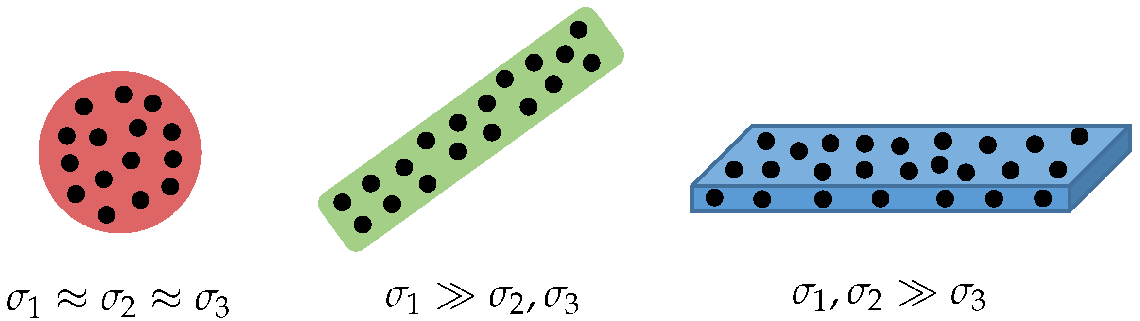
- We propose a surface analysis technique that is used to build a topological space on top of the point cloud, providing for each point its ideal neighborhood and taking into account the underlying surface.
- We keep track of a global 3D map that is continuously updated by means of a surface reconstruction technique that allows us to resample the point cloud. This way, the global 3D map is continuously improved, i.e., the noise is reduced, and the alignment of the following point clouds can be conducted more accurately.
- The topological space is used to compute low-level features, which will be incorporated in an adapted version of the ICP algorithm to make this latter more robust. The alignment of consecutive local point clouds, as well as the alignment of a local point cloud with the global 3D map will be conducted using this improved ICP algorithm.
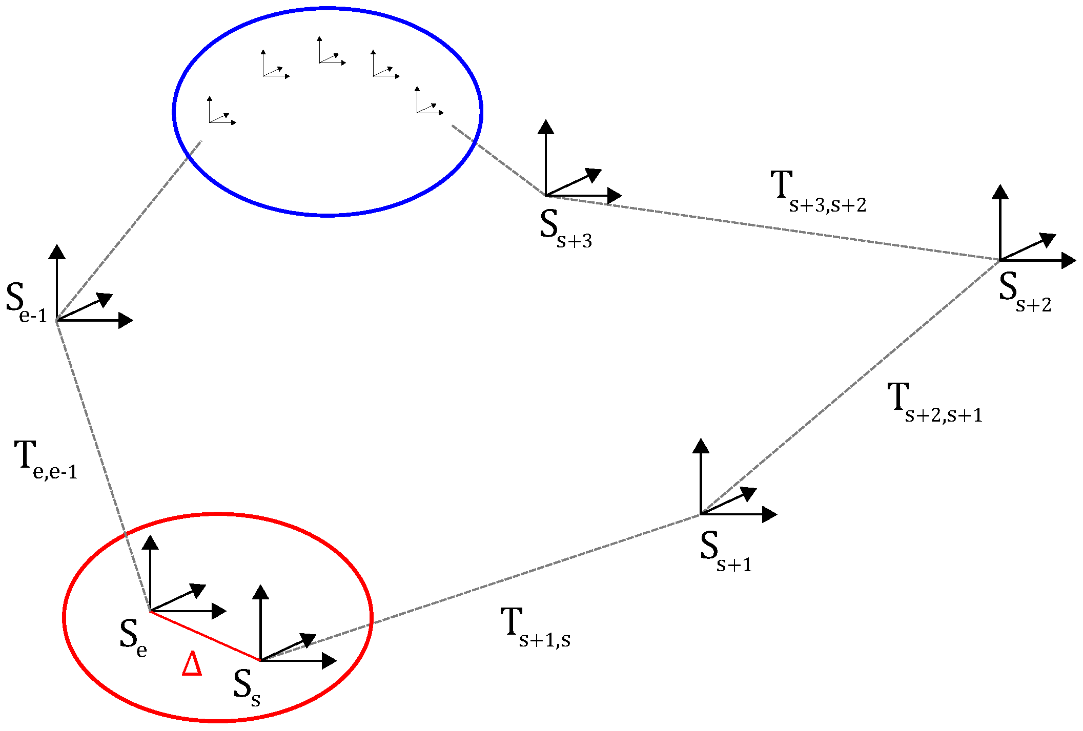
- We incorporate the residual of the ICP process in the loop closure process. Based on this residual, we can predict the share of each pose estimation in the final pose error when a loop has been detected.
2. Related Work
3. System
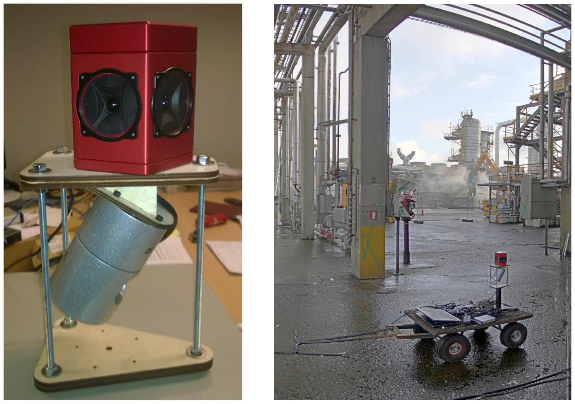
3.1. Acquisition Platform
3.2. Terminology
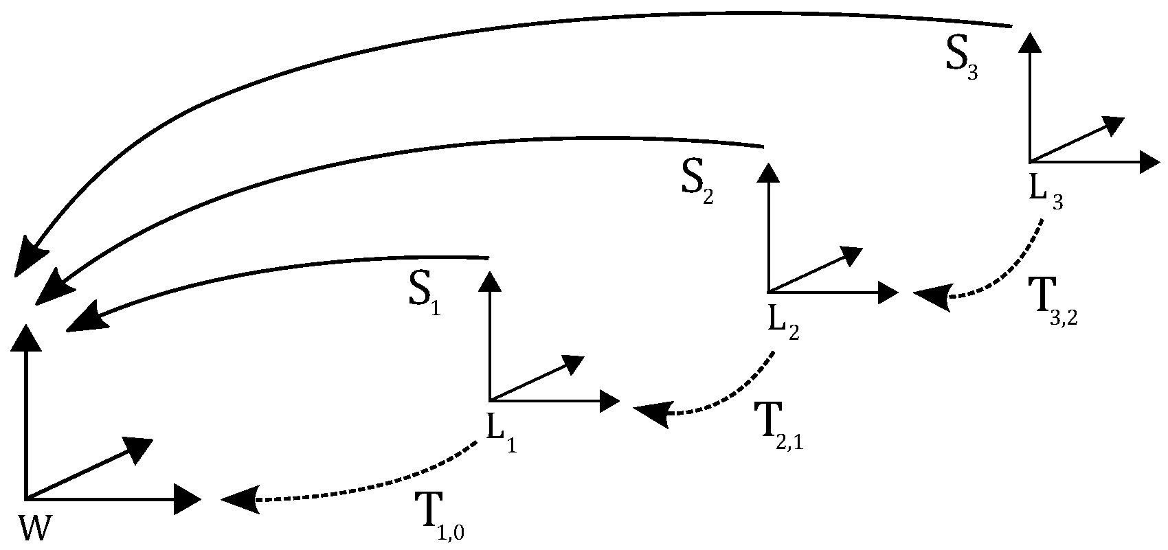
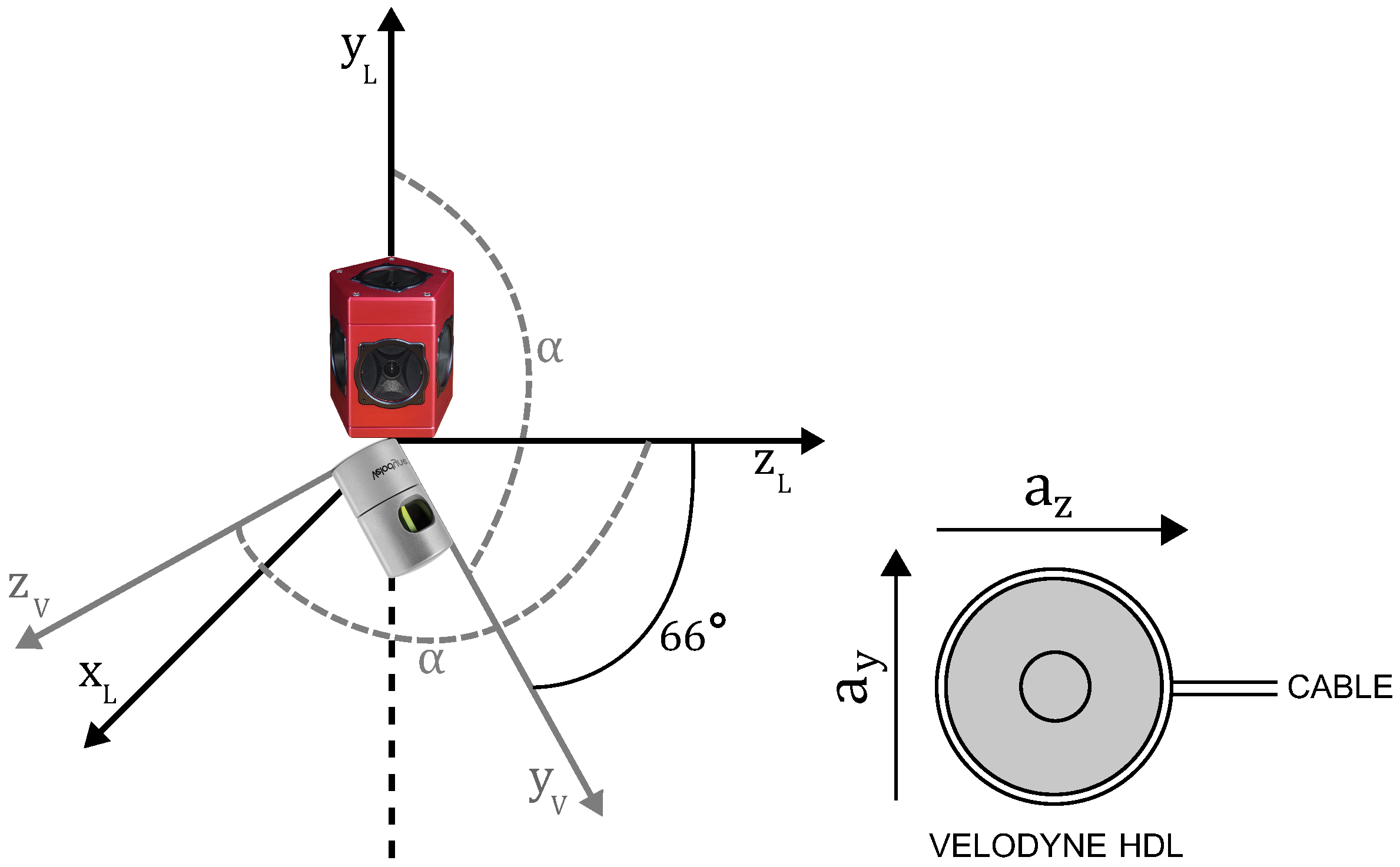
3.3. Reference Coordinate System
3.4. Problem Statement
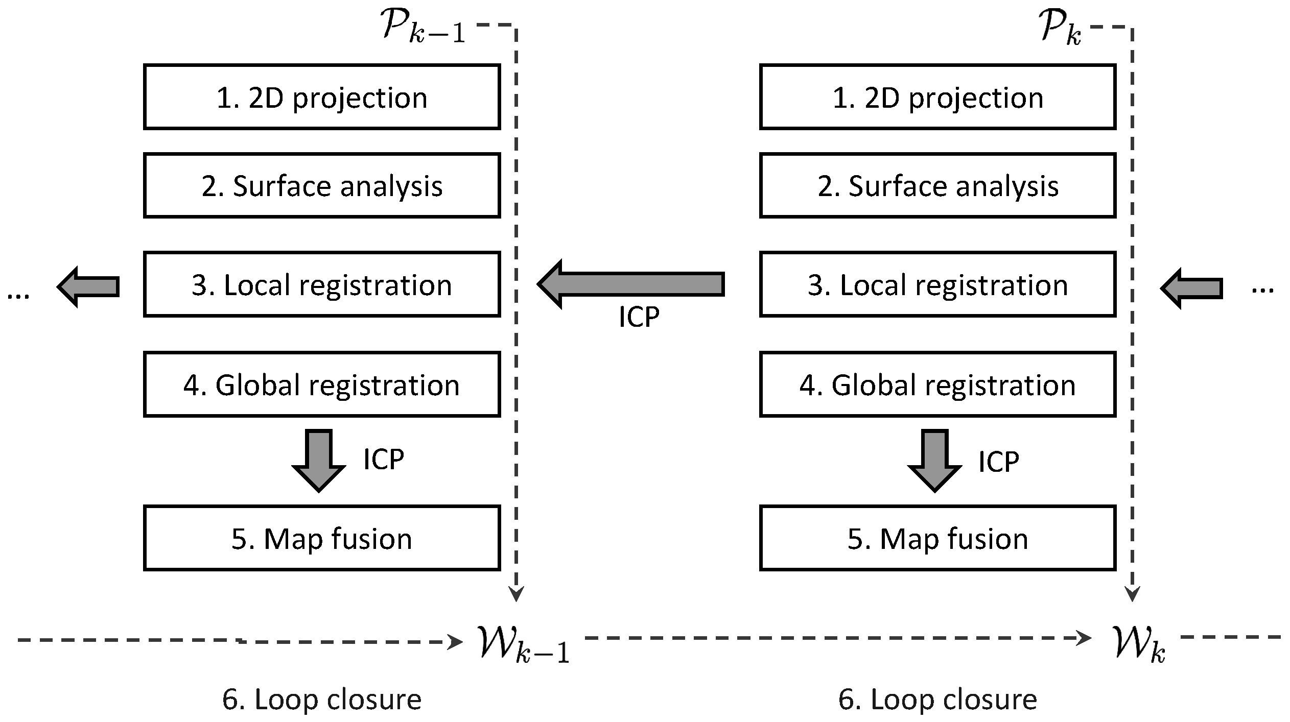
4. Approach
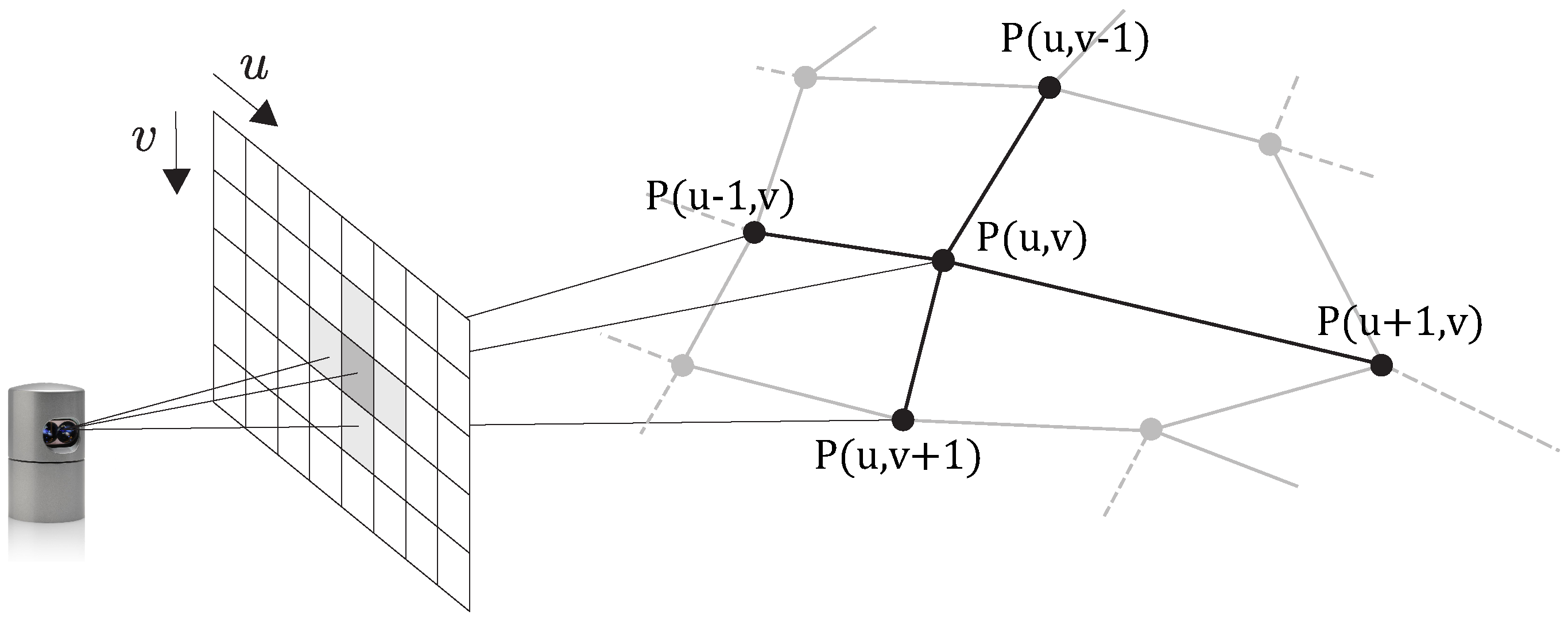
4.1. 2D Projection
4.2. Surface Analysis
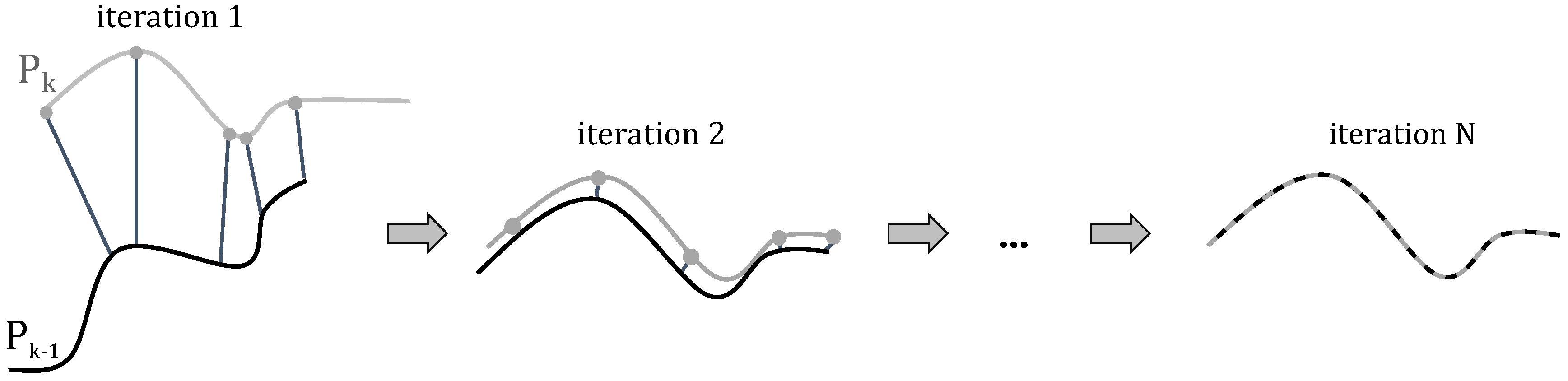
4.3. Local Registration
4.4. Global Registration
4.5. Map Fusion
4.6. Loop Closure
5. Evaluation
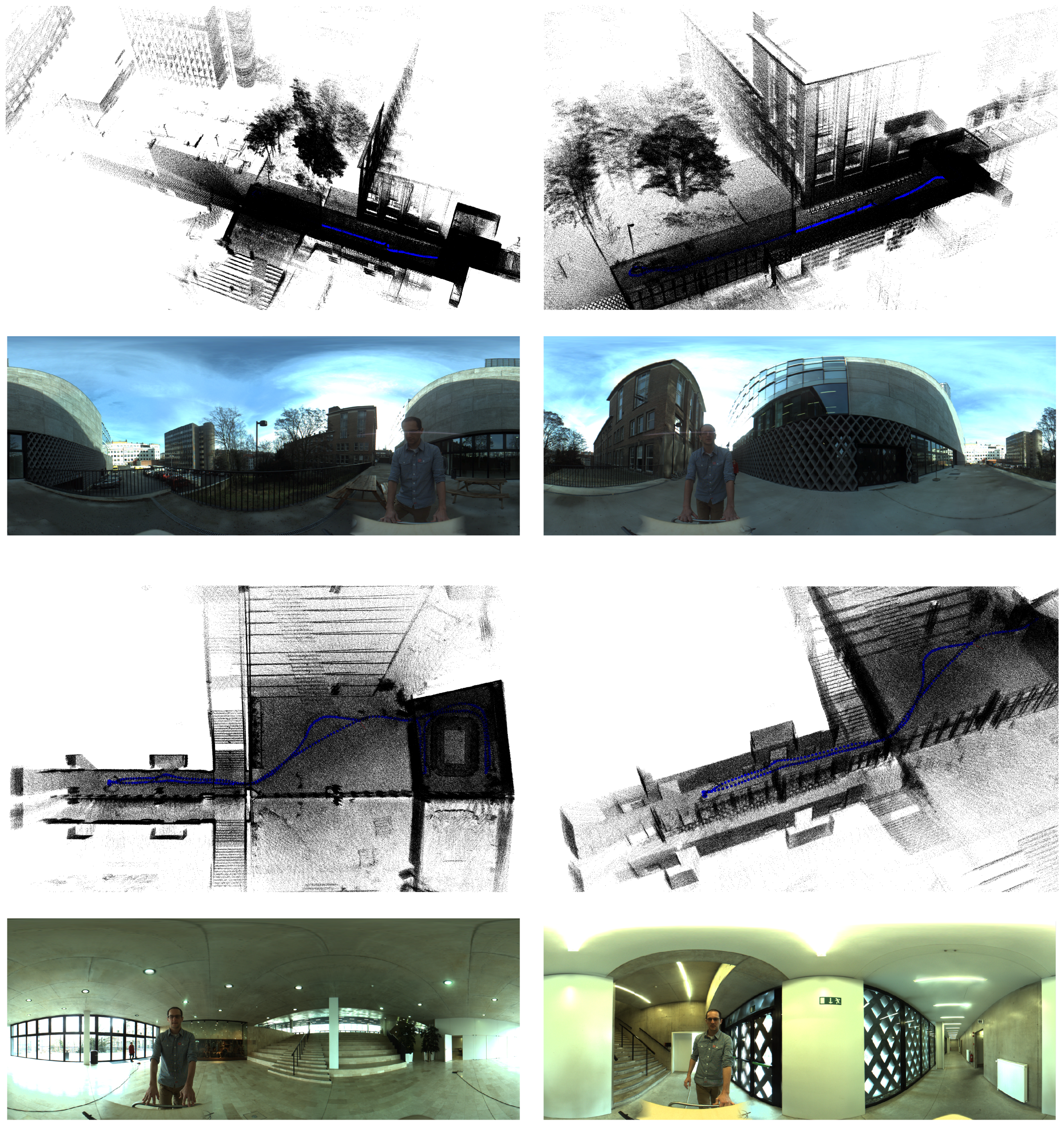
5.1. Our Dataset
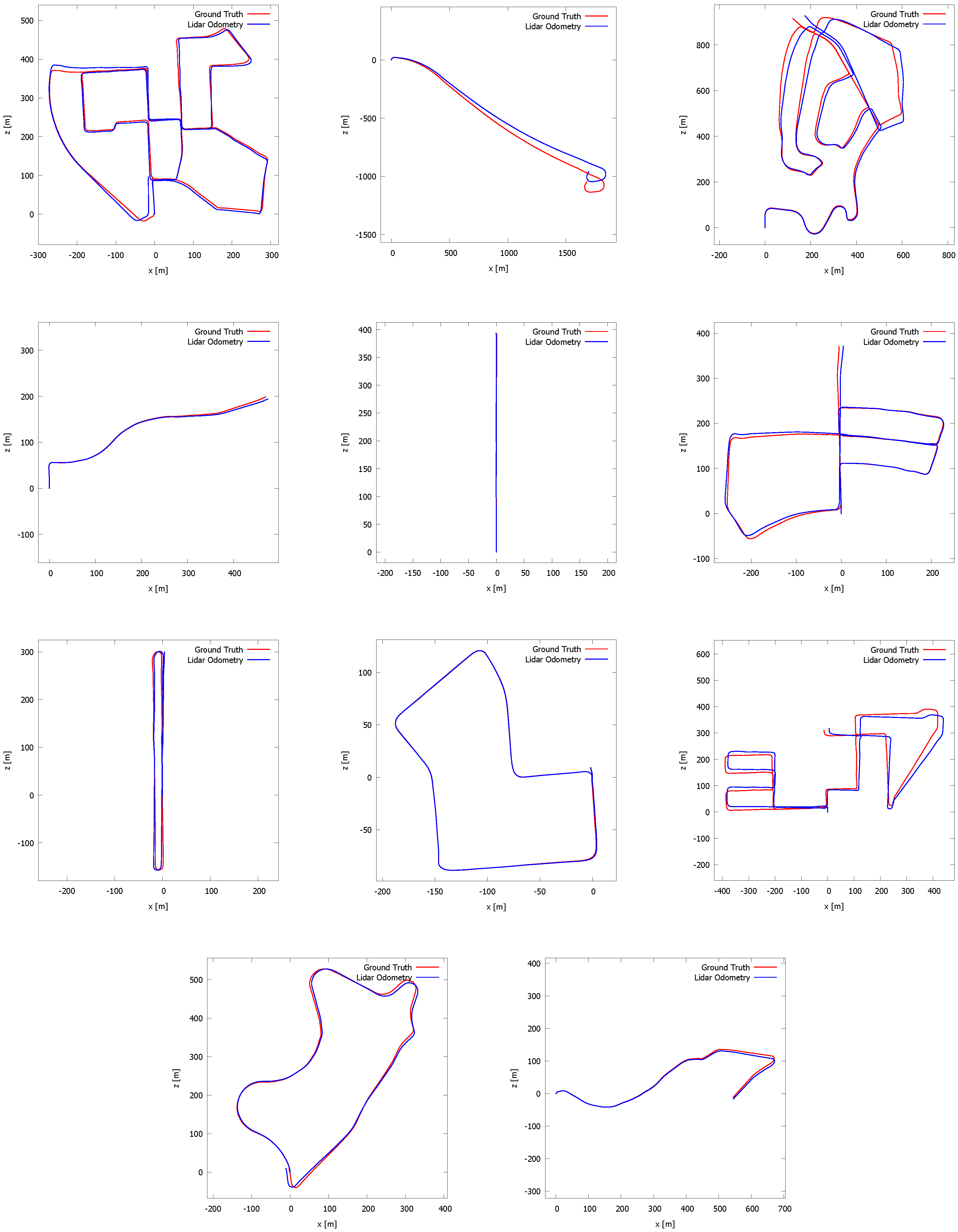
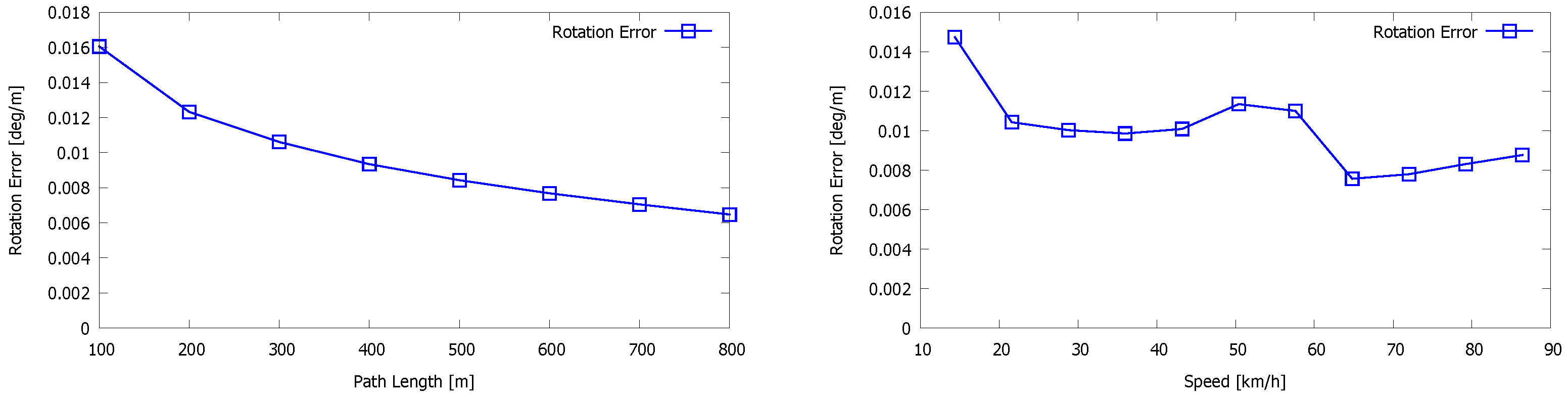
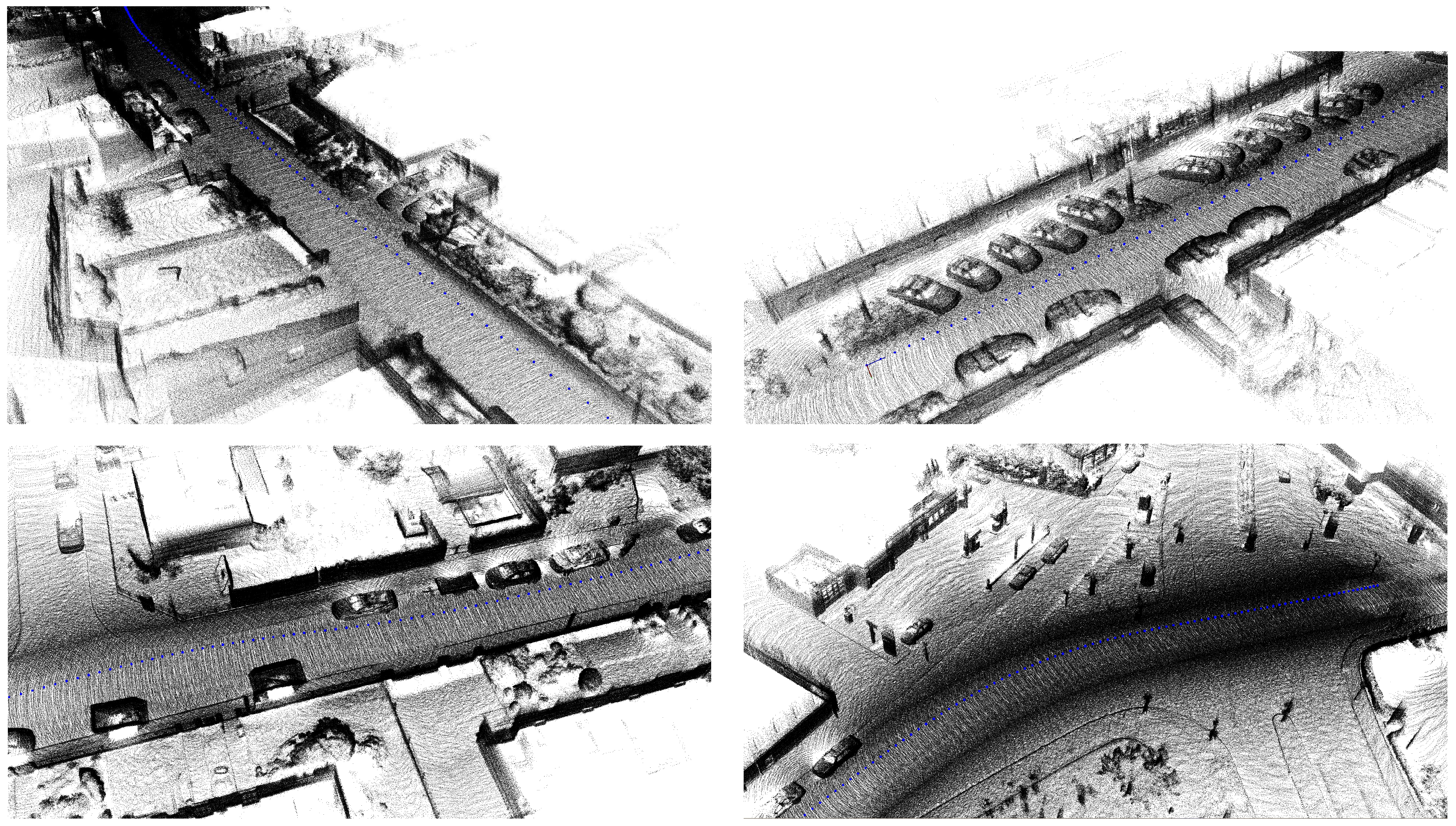
5.2. Kitti Vision Benchmark
6. Conclusions
Acknowledgments
Author Contributions
Conflicts of Interest
References
- Mur-Artal, R.; Montiel, J.M.M.; Tardós, J.D. ORB-SLAM: A Versatile and Accurate Monocular SLAM System. IEEE Trans. Robot. 2015, 31, 1147–1163. [Google Scholar] [CrossRef]
- Caruso, D.; Engel, J.; Cremers, D. Large-Scale direct SLAM for omnidirectional cameras. In Proceedings of the 2015 IEEE/RSJ International Conference on Intelligent Robots and Systems (IROS), Hamburg, Germany, 28 September–2 October 2015; pp. 141–148.
- Billings, S.D.; Boctor, E.M.; Taylor, R.H. Iterative Most-Likely Point Registration (IMLP): A Robust Algorithm for Computing Optimal Shape Alignment. PLoS ONE 2015, 10, e0117688. [Google Scholar] [CrossRef] [PubMed]
- Pomerleau, F.; Colas, F.; Siegwart, R.; Magnenat, S. Comparing ICP Variants on Real-world Data Sets. Auton. Robot. 2013, 34, 133–148. [Google Scholar] [CrossRef]
- Han, J.; Yin, P.; He, Y.; Gu, F. Enhanced ICP for the Registration of Large-Scale 3D Environment Models: An Experimental Study. Sensors 2016, 16, 228. [Google Scholar] [CrossRef] [PubMed]
- Zlot, R.; Bosse, M. Efficient Large-Scale 3D Mobile Mapping and Surface Reconstruction of an Underground Mine. Field Serv. Robot. 2012, 92, 479–493. [Google Scholar]
- Bosse, M.; Zlot, R.; Flick, P. Zebedee: Design of a Spring-Mounted 3-D Range Sensor with Application to Mobile Mapping. IEEE Trans. Robot. 2012, 28, 1104–1119. [Google Scholar] [CrossRef]
- Nüchter, A.; Lingemann, K.; Hertzberg, J.; Surmann, H. 6D SLAM—3D Mapping Outdoor Environments: Research Articles. J. Field Robot. 2007, 24, 699–722. [Google Scholar] [CrossRef]
- Hong, S.; Ko, H.; Kim, J. VICP: Velocity updating iterative closest point algorithm. In Proceedings of the 2010 IEEE International Conference on Robotics and Automation (ICRA), Anchorage, Alaska, 3–8 May 2010; pp. 1893–1898.
- Gressin, A.; Mallet, C.; Demantké, J.; David, N. Towards 3D LiDAR point cloud registration improvement using optimal neighborhood knowledge. ISPRS J. Photogramm. Remote Sens. 2013, 79, 240–251. [Google Scholar] [CrossRef]
- Moosmann, F.; Stiller, C. Velodyne SLAM. In Proceedings of the IEEE Intelligent Vehicles Symposium, Baden-Baden, Germany, 5–9 June 2011; pp. 393–398.
- Sarvrood, Y.B.; Hosseinyalamdary, S.; Gao, Y. Visual-LiDAR Odometry Aided by Reduced IMU. ISPRS Int. J. Geo Inf. 2016, 5. [Google Scholar] [CrossRef]
- Segal, A.; Hähnel, D.; Thrun, S. Generalized-ICP. In Robotics: Science and Systems; Trinkle, J., Matsuoka, Y., Castellanos, J.A., Eds.; The MIT Press: Cambridge, MA, USA, 2009. [Google Scholar]
- Biber, P.; Straßer, W. The normal distributions transform: A new approach to laser scan matching. In Proceedings of the IEEE/RSJ International Conference on Intelligent Robots and Systems (IROS), Las Vegas, NV, USA, 27 October–1 November 2003; pp. 2743–2748.
- Sun, Y.X.; Li, J.L. Mapping of Rescue Environment Based on NDT Scan Matching. In Proceedings of the 2nd International Conference on Computer Science and Electronics Engineering (ICCSEE 2013), Hangzhou, China, 22–23 March 2013; Volume 760, pp. 928–933.
- Magnusson, M.; Lilienthal, A.; Duckett, T. Scan registration for autonomous mining vehicles using 3D-NDT. J. Field Robot. 2007, 24, 803–827. [Google Scholar] [CrossRef]
- Einhorn, E.; Gross, H.M. Generic NDT Mapping in Dynamic Environments and Its Application for Lifelong SLAM. Robot. Auton. Syst. 2015, 69, 28–39. [Google Scholar] [CrossRef]
- Zhang, J.; Singh, S. LOAM: LiDAR Odometry and Mapping in Real-time. In Proceedings of the Robotics: Science and Systems Conference (RSS), Berkeley, CA, USA, 13–15 July 2014.
- Zhang, J.; Singh, S. Visual-LiDAR Odometry and Mapping: Low-drift, Robust, and Fast. In Proceedings of the IEEE International Conference on Robotics and Automation (ICRA), Seattle, Washington, DC, USA, 26–30 May 2015.
- Pathak, K.; Birk, A.; Vaskevicius, N.; Poppinga, J. Fast Registration Based on Noisy Planes with Unknown Correspondences for 3D Mapping. IEEE Trans. Robot. 2010, 26, 424–441. [Google Scholar] [CrossRef]
- Grant, W.; Voorhies, R.; Itti, L. Finding Planes in LiDAR Point Clouds for Real-Time Registration. In Proceedings of the IEEE/RSJ International Conference on Intelligent Robots and Systems (IROS), Tokyo, Japan, 3–7 November 2013; pp. 4347–4354.
- Xiao, J.; Adler, B.; Zhang, J.; Zhang, H. Planar Segment Based Three-dimensional Point Cloud Registration in Outdoor Environments. J. Field Robot. 2013, 30, 552–582. [Google Scholar] [CrossRef]
- Low, K.L. Linear Least-Squares Optimization for Point-to Plane ICP Surface Registration; Technical Report 4; University of North Carolina: Chapel Hill, NC, USA, 2004. [Google Scholar]
- Levin, D. The Approximation Power of Moving Least-squares. Math. Comput. 1998, 67, 1517–1531. [Google Scholar] [CrossRef]
- Galvez-Lopez, D.; Tardos, J.D. Bags of Binary Words for Fast Place Recognition in Image Sequences. IEEE Trans. Robot. 2012, 28, 1188–1197. [Google Scholar] [CrossRef]
- Shoemake, K. Animating Rotation with Quaternion Curves. SIGGRAPH Comput. Graph. 1985, 19, 245–254. [Google Scholar] [CrossRef]
- Geiger, A.; Lenz, P.; Urtasun, R. Are we ready for Autonomous Driving? The KITTI Vision Benchmark Suite. In Proceedings of the Conference on Computer Vision and Pattern Recognition (CVPR), Providence, RI, USA, 16–21 June 2012.
- Wu, C. Towards Linear-Time Incremental Structure from Motion. In Proceedings of the 2013 International Conference on 3D Vision, Sydney, Australia, 1–8 December 2013; pp. 127–134.


| Sensor | Feature | |
|---|---|---|
 | Ladybug system | - 6 camera’s in pentagonal prism, one pointing upwards |
| - resolution of 1600 × 1200 per image | ||
| - 1 frame (6 images) per second | ||
| - mounted perpendicular w.r.t. the ground plane | ||
 | Velodyne HDL-32e | - 360 horizontal FOV, 41.3 vertical FOV |
| - 32 lasers spinning at 10 sweeps per second | ||
| - ±700,000 points per sweep | ||
| - mounted with an angle of 66 w.r.t. the ground plane |
| Plane | ||
|---|---|---|
| 1 | 0.759761 | 0.00818437 |
| 2 | 0.276246 | 0.00724192 |
| 3 | 1.12969 | 0.008299 |
| 4 | 0.286674 | 0.0115731 |
| 5 | 0.292083 | 0.0164202 |
| 6 | 0.492578 | 0.0106246 |
| 7 | 1.80667 | 0.0118678 |
| 8 | 1.68458 | 0.00993411 |
© 2016 by the authors; licensee MDPI, Basel, Switzerland. This article is an open access article distributed under the terms and conditions of the Creative Commons Attribution (CC-BY) license (http://creativecommons.org/licenses/by/4.0/).
Share and Cite
Vlaminck, M.; Luong, H.; Goeman, W.; Philips, W. 3D Scene Reconstruction Using Omnidirectional Vision and LiDAR: A Hybrid Approach. Sensors 2016, 16, 1923. https://doi.org/10.3390/s16111923
Vlaminck M, Luong H, Goeman W, Philips W. 3D Scene Reconstruction Using Omnidirectional Vision and LiDAR: A Hybrid Approach. Sensors. 2016; 16(11):1923. https://doi.org/10.3390/s16111923
Chicago/Turabian StyleVlaminck, Michiel, Hiep Luong, Werner Goeman, and Wilfried Philips. 2016. "3D Scene Reconstruction Using Omnidirectional Vision and LiDAR: A Hybrid Approach" Sensors 16, no. 11: 1923. https://doi.org/10.3390/s16111923
APA StyleVlaminck, M., Luong, H., Goeman, W., & Philips, W. (2016). 3D Scene Reconstruction Using Omnidirectional Vision and LiDAR: A Hybrid Approach. Sensors, 16(11), 1923. https://doi.org/10.3390/s16111923