
Modelling of XCO2 Surfaces Based on Flight Tests of TanSat Instruments


 ,
, 
Abstract
:1. Introduction
2. Study Area and Data
2.1. Flight Logistics and Data
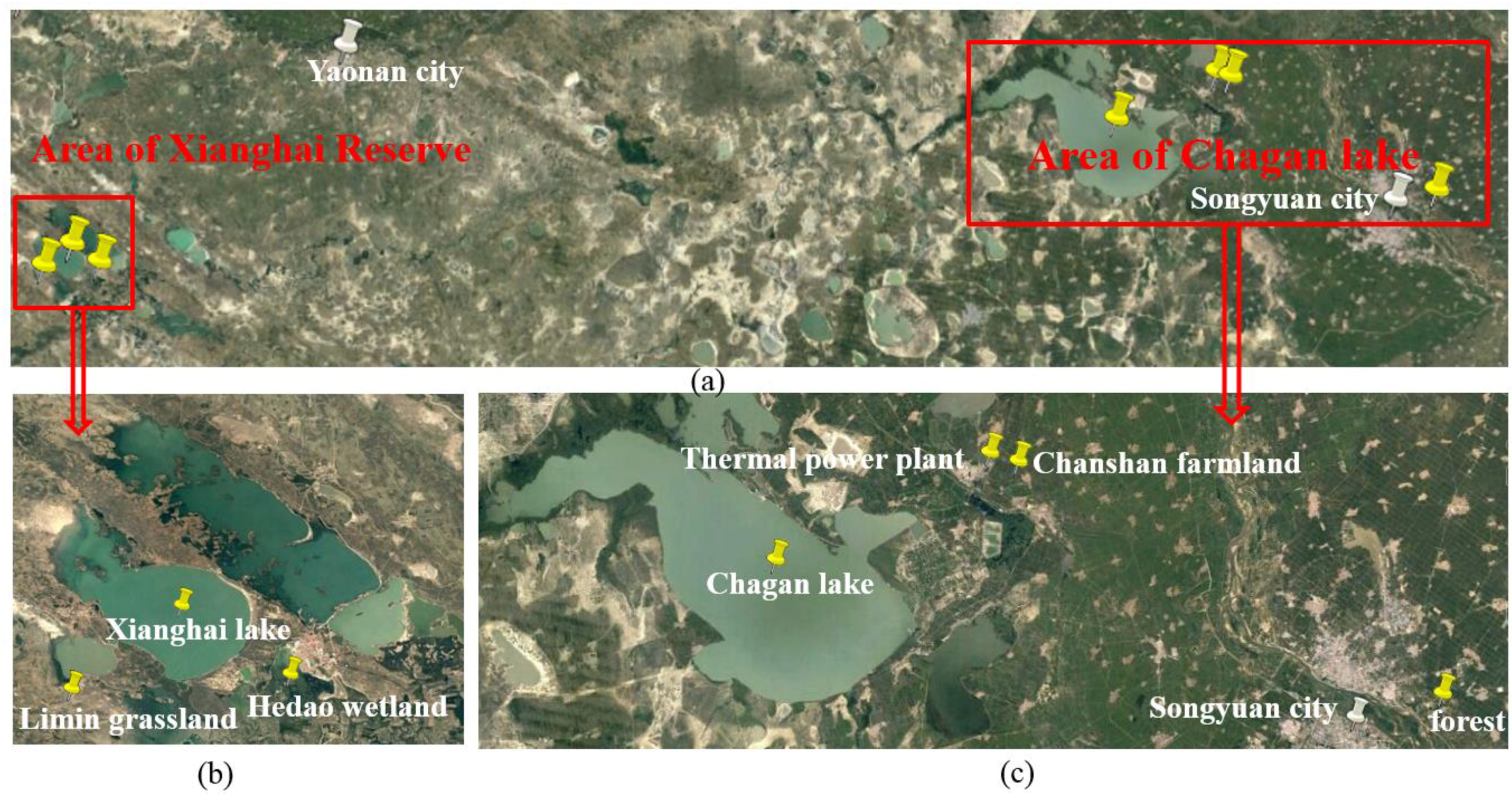
2.2. Study Area and Surface Characteristics
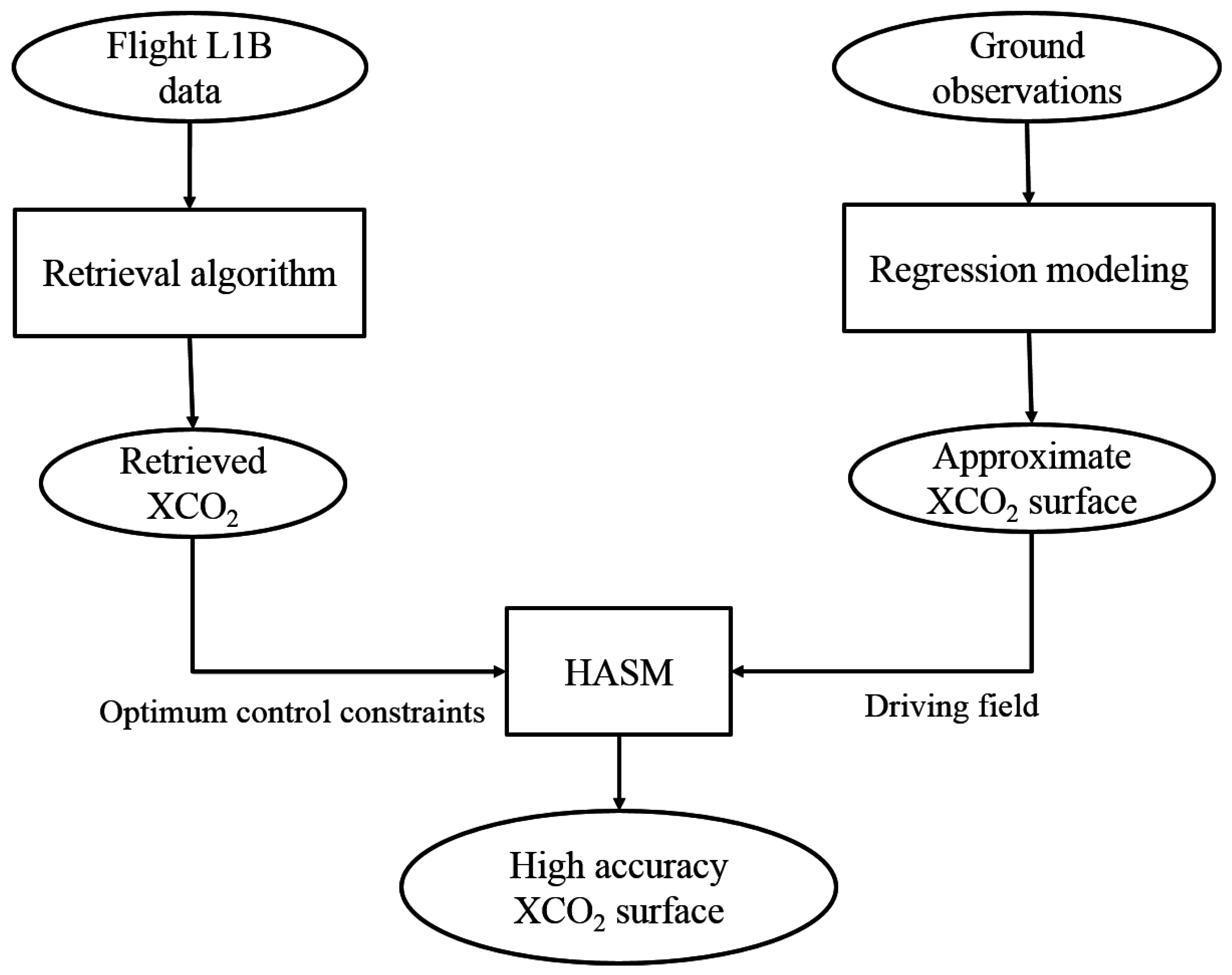
3. Methods
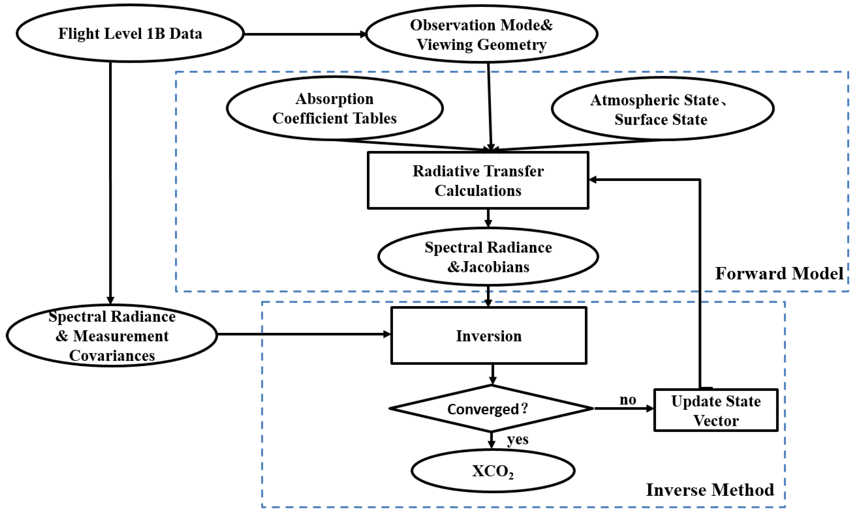
3.1. Retrieval Algorithm
3.1.1. Forward Model
3.1.2. Inverse Method
- (1)
- (2)
- The normalized successive difference of the state vector is less than some pre-determined threshold (1%) in the TANSO-FTS SWIR L2 algorithm (see [2] for details).
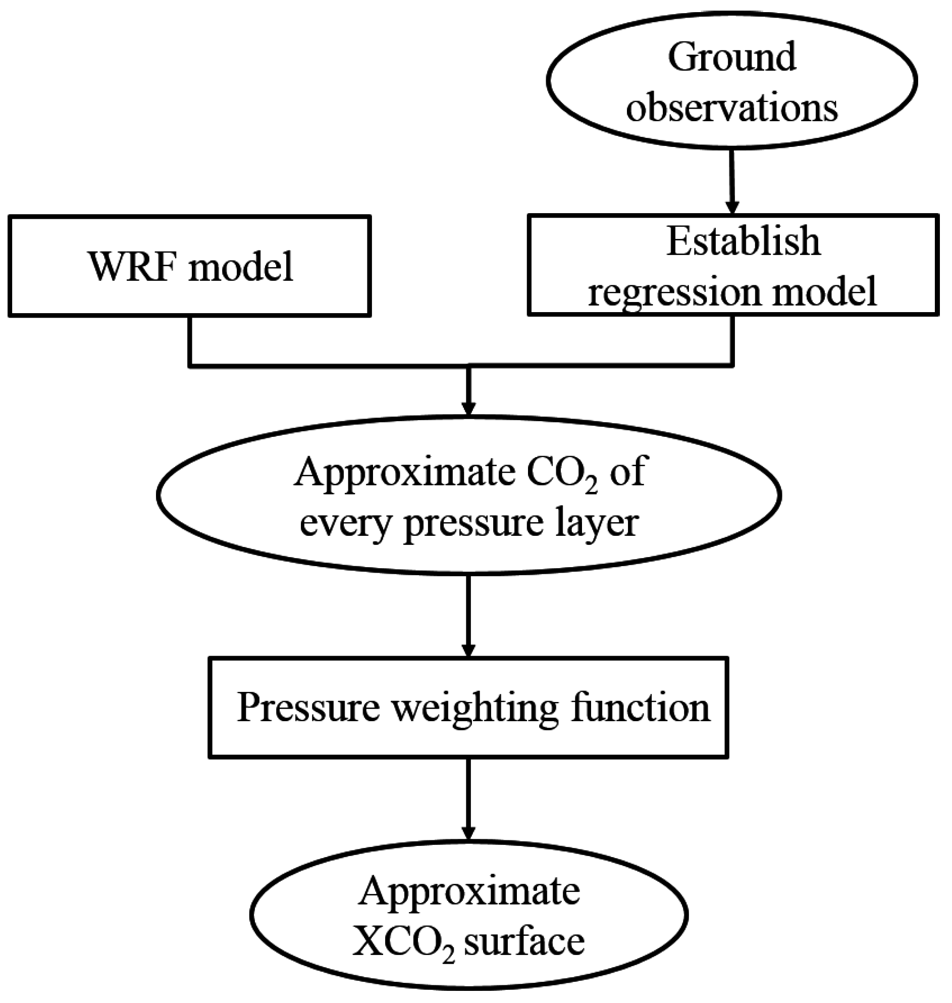
3.2. Derivation of Approximate XCO2 Surface
3.2.1. Initial Regression Model
3.2.2. WRF Model
3.2.3. Pressure Weighting Function
3.3. High Accuracy Surface Modeling
4. Results
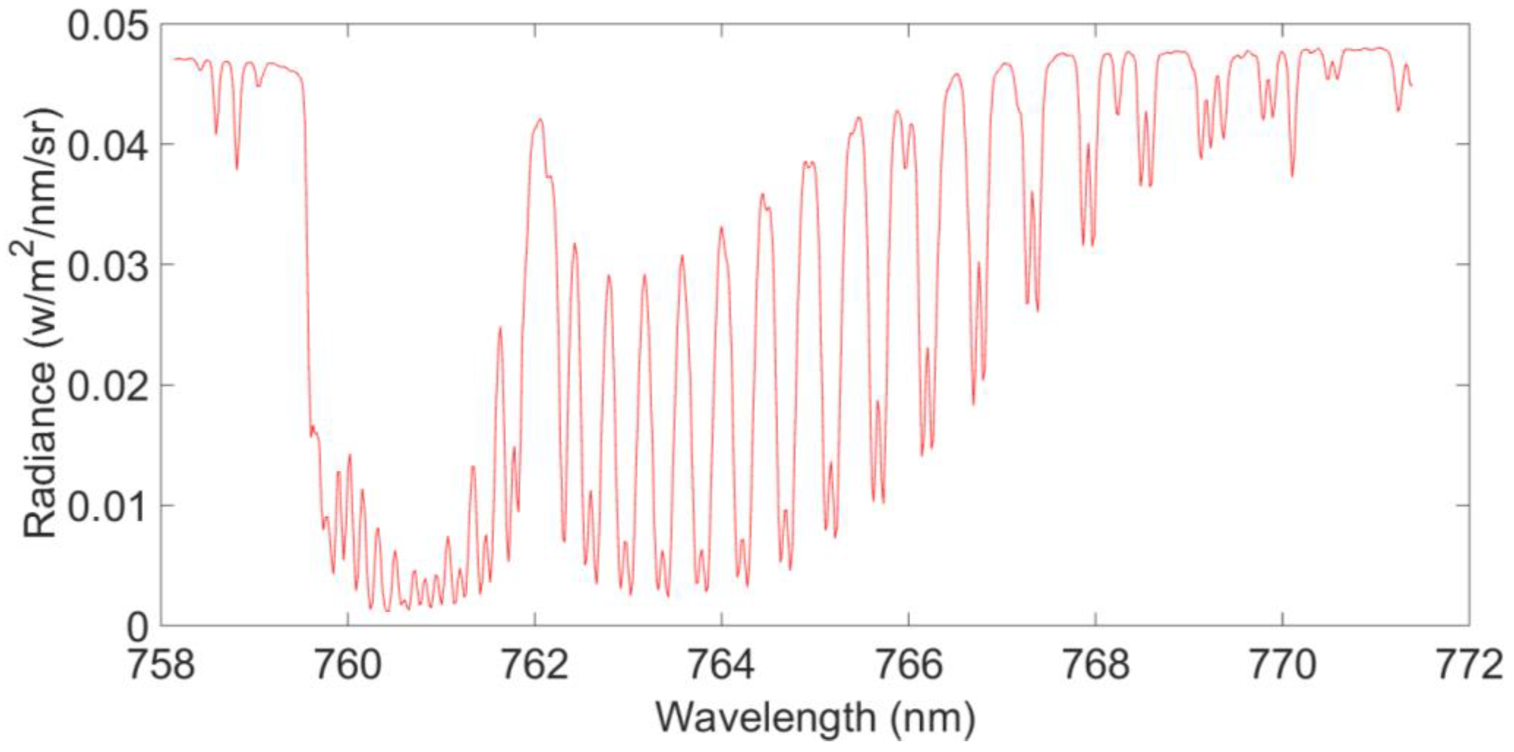
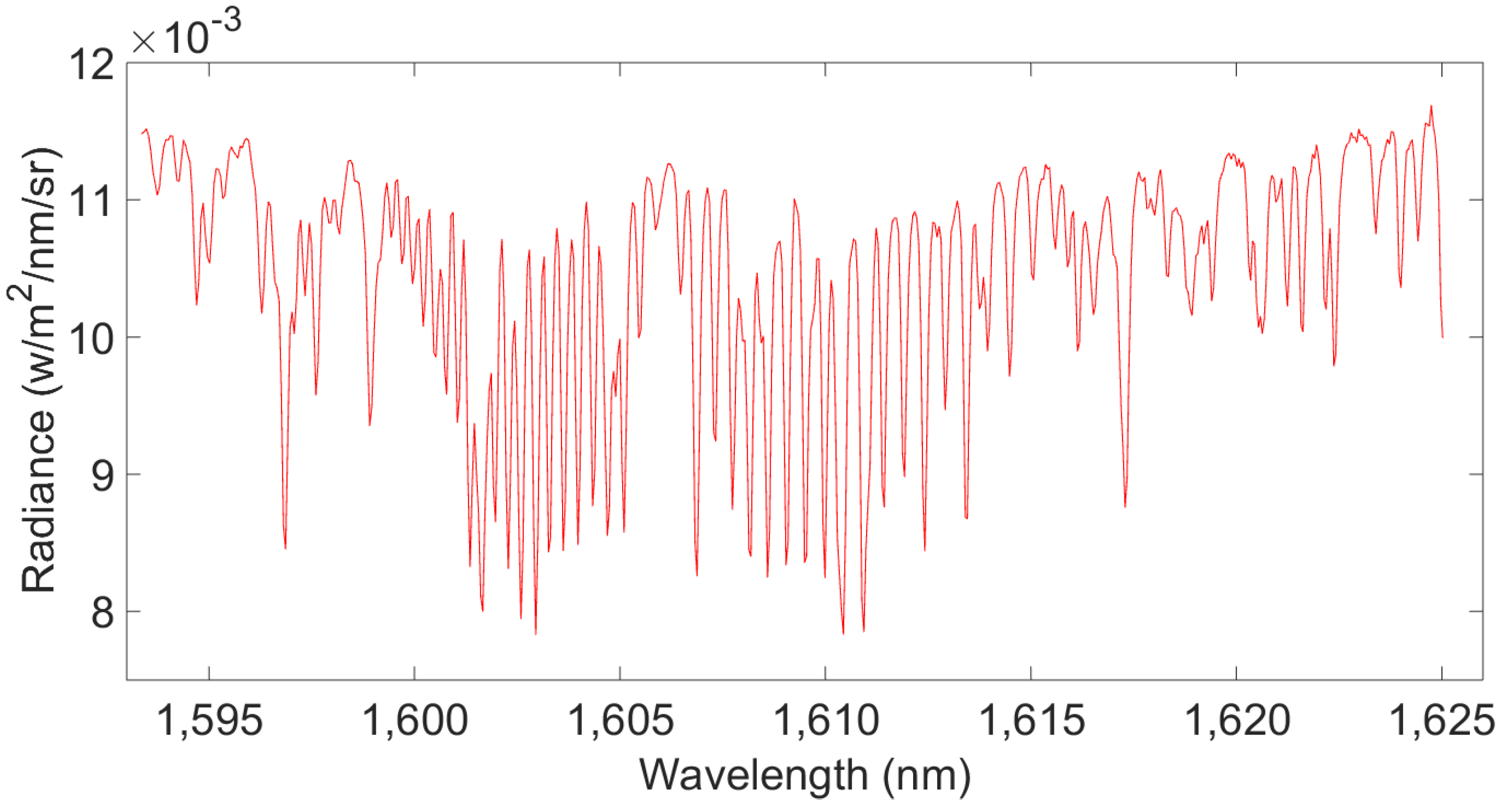
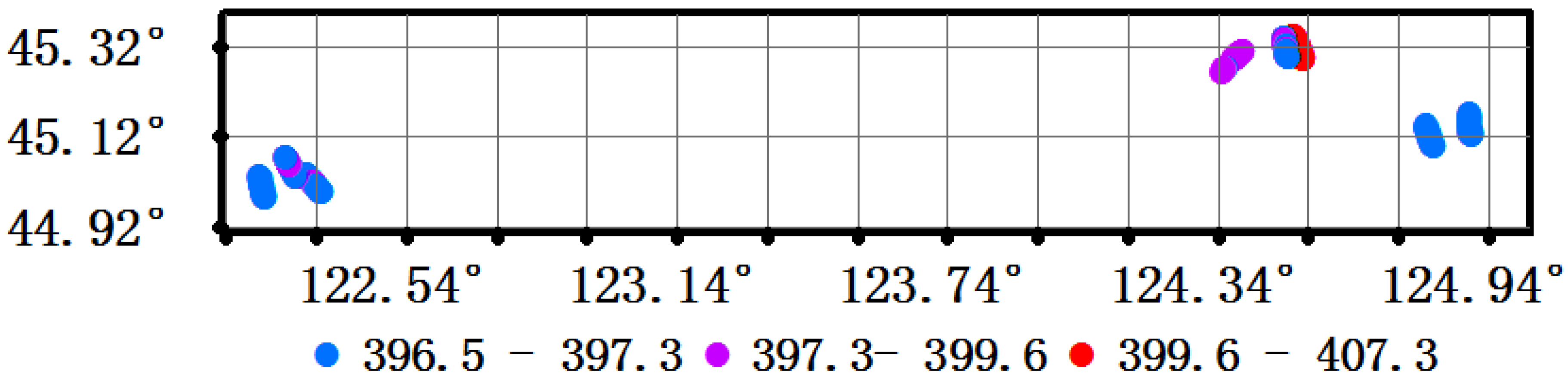
4.1. Retrieval XCO2
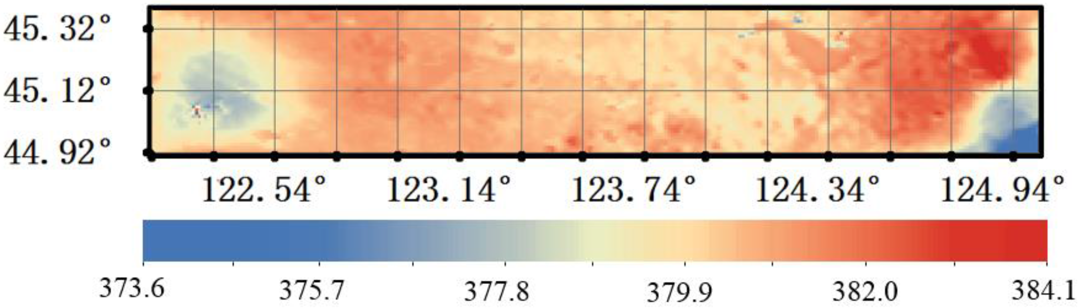
4.2. Approximate XCO2 Surface in the Flight Test Area
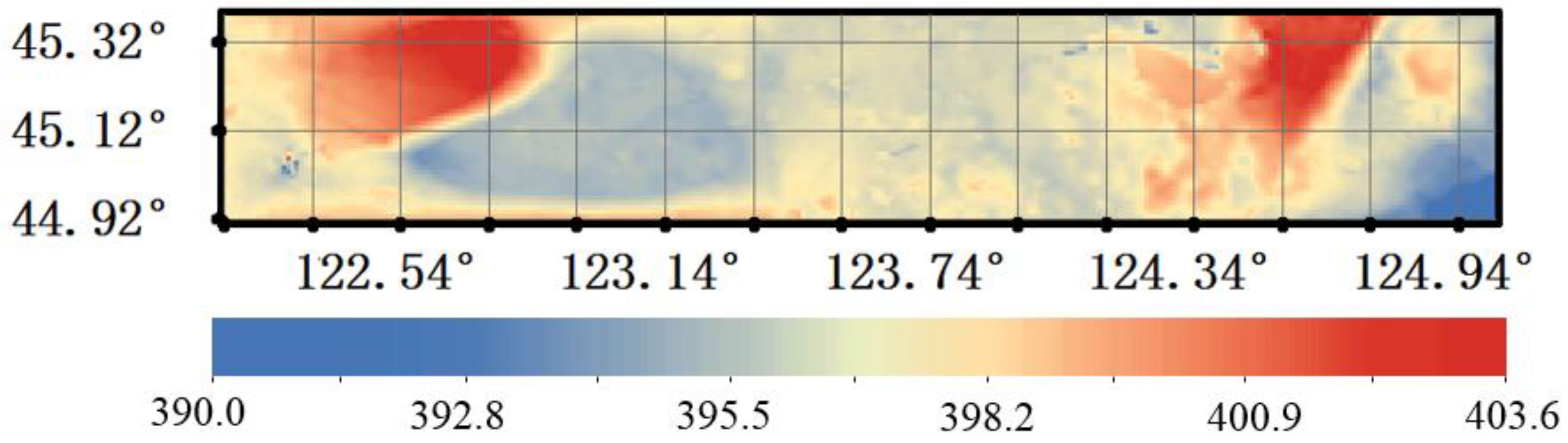
4.3. High Accuracy XCO2 Surface
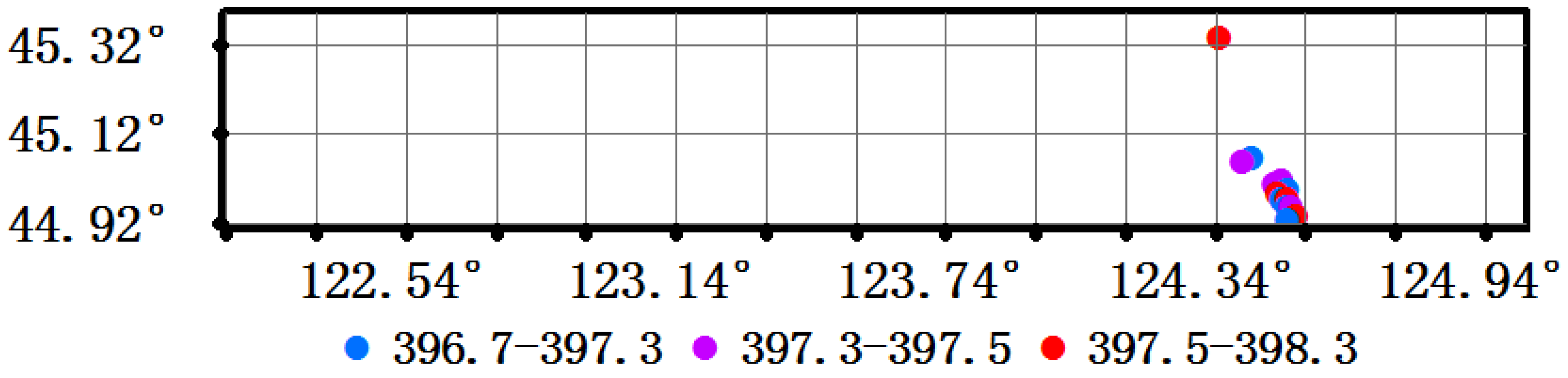
4.4. Comparison with OCO-2’s XCO2 Estimates
5. Conclusions
Acknowledgments
Author Contributions
Conflicts of Interest
References
- Meehl, G.A.; Washington, W.M. El Nino-like climate change in a model with increased atmospheric CO2 concentrations. Nature 1996, 382, 56–60. [Google Scholar] [CrossRef]
- Yoshida, Y.; Ota1, Y.; Eguchi1, N.; Kikuchi, N.; Nobuta, K.; Tran, H.; Morino1, I.; Yokota, T. Retrieval algorithm for CO2 and CH4 column abundances from short-wavelength infrared spectral observations by the Greenhouse gases observing satellite. Atmos. Meas. Tech. 2011, 4, 717–734. [Google Scholar] [CrossRef]
- Oshchepkov, S.; Bril, A.; Maksyutov, S.; Yokota, T. Detection of optical path in spectroscopic space-based observations of greenhouse gases: Application to GOSAT data processing. J. Geophys. Res. 2011, 116, D14304. [Google Scholar] [CrossRef]
- Schneising, O.; Buchwitz, M.; Burrows, J.P.; Bovensmann, H.; Reuter, M.; Notholt, J.; Macatangay, R.; Warneke, T. Three years of greenhouse gas column-averaged dry air mole fractions retrieved from satellite—Part 1: Carbon dioxide. Atmos. Meas. Tech. 2008, 8, 3827–3853. [Google Scholar] [CrossRef]
- Guerlet, S.; Butz, A.; Schepers, D.; Basu, S.; Hasekamp, O.P.; Kuze, A.; Yokota, T.; Blavier, J.F.; Deutscher, N.M.; Griffith, D.W.T.; et al. Impact of aerosol and thin cirrus on retrieving and validating XCO2 from GOSAT shortwave infrared measurements. J. Geophys. Res. 2013, 118, 4887–4905. [Google Scholar]
- Boesch, H.; Toon, G.C.; Sen, B.; Washenfelder, R.A.; Wennberg, P.O.; Buchwitz, M.; Beek, R.D.; Burrows, J.P.; Crisp, D.; Christi, M.; et al. Space-Based near-infrared CO2 measurements: Testing the Orbiting Carbon Observatory retrieval algorithm and validation concept using SCIAMACHY observations over Park Falls, Wisconsin. J. Geophys. Res. 2006, 111, D23302. [Google Scholar]
- Boesch, H.; Baker, D.; Connor, B.; Crisp, D.; Miller, C. Characterization of CO2 Column Retrievals from Shortwave-Infrared Satellite Observations of the Orbiting Carbon Observatory-2 Mission. Remote Sens. 2011, 3, 270–304. [Google Scholar] [CrossRef]
- Connor, B.J.; Boesch, H.; Toon, G.; Sen, B.; Miller, C.; Crisp, D. Orbiting Carbon Observatory: Inverse method and prospective error analysis. J. Geophys. Res. Atmos. 2008, 113, D05305. [Google Scholar] [CrossRef]
- O’Dell, C.W.; Connor, B.; Boesch, H.; O’Brien, D.; Frankenberg, C.; Castano, R.; Christi, M.; Eldering, D.; Fisher, B.; Gunson, M.; et al. The ACOS CO2 retrieval algorithm—Part 1: Description andvalidation against synthetic observations. Atmos. Meas. Tech. 2012, 5, 99–121. [Google Scholar] [CrossRef]
- Bovensmann, H.; Buchwitz, M.; Burrows, J.P.; Reuter, M.; Krings, T.; Gerilowski, K.; Schneising, O.; Heymann, J.; Tretner, A.; Erzinger, J. A remote sensing technique for global monitoring of power plant CO2 emissions from space and related applications. Atmos. Meas. Tech. 2010, 3, 781–811. [Google Scholar] [CrossRef]
- Reuter, M.; Buchwitz, M.; Schneising, O.; Heymann, J.; Bovensmann, H.; Burrows, J.P. A method for improved SCIAMACHY CO2 retrieval in the presence of optically thin clouds. Atmos. Meas. Tech. 2009, 2, 2483–2538. [Google Scholar] [CrossRef]
- Schneising, O.; Bergamaschi, P.; Bovensmann, H.; Buchwitz, M.; Burrows, J.P.; Deutscher, N.M.; Griffith, D.W.T.; Heymann, J.; Macatangay, R.; Messerschmidt, J.; et al. Atmospheric greenhouse gases retrieved from SCIAMACHY: Comparison to ground-based FTS measurements and model results. Atmos. Meas. Tech. 2012, 12, 1527–1540. [Google Scholar] [CrossRef]
- Reuter, M.; Bovensmann, H.; Buchwitz, M.; Burrows, J.P.; Connor, B.J.; Deutscher, N.M.; Griffith, D.W.T.; Heymann, J.; Aleks, G.K.; Messerschmidt, J.; et al. Retrieval of atmospheric CO2 with enhanced accuracy and precision from SCIAMACHY: Validation with FTS measurements and comparison with model results. J. Geophys. Res. 2011, 116, D04301. [Google Scholar] [CrossRef]
- Heymann, J.; Reuter, M.; Hilker, M.; Buchwitz, M.; Schneising, O.; Bovensmann, H.; Burrows, J.P.; Kuze, A.; Suto, H.; Deutscher, N.M.; et al. Consistent satellite XCO2 retrievals from SCIAMACHY and GOSAT using the BESD algorithm. Atmos. Meas. Tech. 2015, 8, 2961–2980. [Google Scholar] [CrossRef]
- Cogan, J.; Boesch, H.; Parker, R.J.; Feng, L.; Palmer, P.I.; Blavier, J.F.L.; Deutscher, N.M.; Macatangay, R.; Notholt, J.; Roehl, C.; et al. Atmospheric carbon dioxide retrieved from the Greenhouse gases Observing SATellite (GOSAT): Comparison with ground-based TCCON observations and GEOS-Chem model calculations. J. Geophys. Res. 2012, 117, D21301. [Google Scholar] [CrossRef]
- Crisp, D.; Fisher, B.M.; O’Dell, C.; Frankenberg, C.; Basilio, R.; Boesch, H.; Brown, L.R.; Castano, R.; Connor, B.; Deutscher, N.; et al. The ACOS CO2 retrieval algorithm—Part II: Global XCO2 data characterization. Atmos. Meas. Tech. 2012, 5, 687–707. [Google Scholar] [CrossRef]
- Wang, C.L.; Zhao, N.; Yue, T.X.; Zhao, M.W.; Chen, C. Change trend of monthly precipitation in China with an improved surface modeling method. Environ. Earth Sci. 2015, 74, 6459–6469. [Google Scholar] [CrossRef]
- Liu, Y.; Guo, J.H.; Yue, T.X.; Zhao, N. Simulation and analysis of carbon dioxide concentration in surface layer. Geo-Inf. Sci. 2016, in press. [Google Scholar]
- Yue, T.X.; Fan, Z.M.; Chen, C.F.; Sun, X.F.; Li, B.L. Surface modeling of global terrestrial ecosystems under three climate change scenarios. Ecol. Model. 2011, 222, 2342–2361. [Google Scholar] [CrossRef]
- Rodgers, C.D. Inverse Methods for Atmospheric Sounding: Theory and Practice; World Scientific Publishing: Singapore, 2000. [Google Scholar]
- Li, W.B. Atmospheric Remote Sensing; Peking University Press: Beijing, China, 2014. [Google Scholar]
- Rozanov, V.V.; Rozanovn, A.V.; Kokhanovsky, A.A.; Burrows, J.P. Radiative transfer through terrestrial atmosphere and ocean: Software package SCIATRAN. J. Quant. Spectrosc. Radiat. Transf. 2014, 133, 13–71. [Google Scholar] [CrossRef]
- Wunch, D.; Toon, G.C.; Jean-François, L.B.; Rebecca, A.W.; Notholt, J.; Connor, B.J.; Griffith, D.W.T.; Sherlock, V.; Wennberg, P.O. The Total Carbon Column Observing Network. Philos. Trans. R. Soc. 2011, 369, 2087–2112. [Google Scholar] [CrossRef] [PubMed]
- Michalakes, J.; Dudhia, J.; Grill, D.; Klemp, J.; Skamarock, W. Design of a next-generation regional weather research and forecast model. In Towards Teracomputing: Proceedings of the Eighth ECMWF Workshop on the Use of Parallel Processors in Meteorology; World Scientific: River Edge, NJ, USA, 1998; pp. 117–124. [Google Scholar]
- Michalakes, J.; Chen, S.; Dudhia, J.; Hart, L.; Klemp, J.; Middlecoff, J.; Skamarock, W. Development of a Next Generation Regional Weather Research and Forecast Model. In Developments in Teracomputing: Proceedings of the Ninth ECMWF Workshop on the Use of High Performance Computing in Meteorology; World Scientific: Singapore, 2001; pp. 269–276. [Google Scholar]
- Yue, T.X. Surface Modelling: High Accuracy and High Speed Methods; CRC Press: Boca Raton, FL, USA, 2011. [Google Scholar]
- Yue, T.X.; Du, Z.P.; Song, D.J.; Gong, Y. A new method of surface modeling and its application to DEM construction. Geomorphology 2007, 91, 161–172. [Google Scholar] [CrossRef]
- Yue, T.X.; Chen, C.F.; Li, B.L. An adaptive method of high accuracy surface modeling and its application to simulating elevation surfaces. Trans. GIS 2010, 14, 615–630. [Google Scholar] [CrossRef]
- Yue, T.X.; Song, D.J.; Du, Z.P.; Wang, W. High-Accuracy surface modelling and its application to DEM generation. Int. J. Remote Sens. 2010, 31, 2205–2226. [Google Scholar] [CrossRef]
- Yue, T.X.; Wang, S.H. Adjustment computation of HASM: A high-accuracy and high-speed method. Int. J. Geogr. Inf. Sci. 2010, 24, 1725–1743. [Google Scholar] [CrossRef]
- Yue, T.X.; Zhang, L.L.; Zhao, N.; Zhao, M.W.; Chen, C.F.; Du, Z.P.; Song, D.J.; Fan, Z.M.; Shi, W.J.; Wang, S.H.; et al. A review of recent developments in HASM. Environ. Earth Sci. 2015, 74, 6541–6549. [Google Scholar] [CrossRef]
- Yue, T.X.; Zhao, N.; Yang, H.; Song, Y.J.; Du, Z.P.; Fan, Z.M.; Song, D.J. The multi-grid method of high accuracy surface modelling and its validation. Trans. GIS 2013, 17, 943–952. [Google Scholar] [CrossRef]
- Yue, T.X.; Zhao, N.; Ramsey, D.; Wang, C.L.; Fan, Z.M.; Chen, C.F.; Lu, Y.M.; Li, B.L. Climate change trend in China, with improved accuracy. Clim. Chang. 2013, 120, 137–151. [Google Scholar] [CrossRef]
- Shi, W.J.; Liu, J.Y.; Song, Y.J.; Du, Z.P.; Chen, C.F.; Yue, T.X. Surface modelling of soil pH. Geoderma 2009, 150, 113–119. [Google Scholar] [CrossRef]
- Shi, W.J.; Liu, J.Y.; Du, Z.P.; Stein, A.; Yue, T.X. Surface modelling of soil properties based on land use information. Geoderma 2011, 162, 347–357. [Google Scholar] [CrossRef]
- Shi, W.J.; Yue, T.X.; Du, Z.P.; Wang, Z.; Li, X.W. Surface modeling of soil antibiotics. Sci. Total Environ. 2016, 543, 609–619. [Google Scholar] [CrossRef] [PubMed]
- Wunch, D.; Wennberg, P.O.; Osterman, G.; Fisher, B.; Naylor, B.; Roehl, C.M.; O’Dell, C.; Mandrake, L.; Viatte, C.; Griffith, D.W.T.; et al. Comparisons of the Orbiting Carbon Observatory-2 (OCO-2) XCO2 measurements with TCCON. Atmos. Meas. Tech. Discuss. 2016. [Google Scholar] [CrossRef]


| Type | Parameters |
|---|---|
| Flight height | 5 km ± 30 m |
| Flight speed | 220 ± 6.6 km/h |
| Flight time | 10:30–13:30 |
| Solar zenith angle | 40°–55° |
| Flight geometric requirements | Flight drift angle is <5°; range of three-axis attitude angle is <2°; route is straight and course deviation is <60 m. |
| Meteorological conditions | Good weather with visibility >10 km. |
| Band 1 | Band 2 | |
|---|---|---|
| Wavelength range (nm) | 758–772 | 1592–1625 |
| Spectral resolution (nm) | 0.044 | 0.13 |
| Observations | Observation Methods Used |
|---|---|
| Temperature profile | Sonde measurement |
| Humidity profile | Sonde measurement |
| Pressure profile | Sonde measurement |
| Wind profile | Sonde measurement |
| CO2 profile | Captive balloon |
| CO2 concentration in surface layer | Greenhouse gases online laser analyzer UGGA |
| Surface reflectance | Analytical Spectral Devices (ASD) spectrometer |
| Aerosol optical depth | Sun photometer CE318 |
| Inputs | Outputs |
|---|---|
| Solar irradiance spectra | Radiance spectrum |
| Gas absorption and scattering cross sections | Jacobians (partial derivatives of the radiance spectrum with respect to each of the state vector elements) |
| Atmospheric state | - |
| Surface state | - |
| Instrument line shape function | - |
| Aerosol optical properties | - |
| Dependent Variables | Explanatory Variables |
|---|---|
| CO2 concentration in surface layer | Surface pressure, atmospheric humidity, atmospheric temperature, soil humidity, soil temperature, upward and downward shortwave radiation, altitude, longitude and latitude |
| CO2 profile (not including surface layer) | Temperature, pressure and humidity profiles, wind speed and direction, latitude and longitude |
| Number | Longitude (°) | Latitude (°) | Flight Test (ppm) | OCO-2 (ppm) | Difference (ppm) |
|---|---|---|---|---|---|
| 1 | 124.35 | 45.34 | 396.67 | 398.34 | −1.67 |
| 2 | 124.40 | 45.06 | 399.13 | 397.54 | 1.59 |
| 3 | 124.42 | 45.07 | 398.85 | 397.07 | 1.78 |
| 4 | 124.47 | 45.01 | 398.05 | 397.35 | 0.70 |
| 5 | 124.48 | 45.00 | 398.36 | 397.49 | 0.87 |
| 6 | 124.48 | 44.99 | 398.05 | 397.84 | 0.21 |
| 7 | 124.49 | 45.02 | 398.75 | 397.42 | 1.33 |
| 8 | 124.49 | 44.98 | 397.82 | 397.25 | 0.57 |
| 9 | 124.50 | 45.00 | 399.01 | 397.23 | 1.78 |
| 10 | 124.50 | 44.98 | 398.73 | 397.63 | 1.10 |
| 11 | 124.50 | 44.96 | 397.99 | 396.73 | 1.26 |
| 12 | 124.50 | 44.93 | 397.24 | 397.04 | 0.20 |
| 13 | 124.51 | 44.96 | 397.92 | 397.29 | 0.63 |
| 14 | 124.52 | 44.94 | 397.35 | 397.87 | −0.52 |
© 2016 by the authors; licensee MDPI, Basel, Switzerland. This article is an open access article distributed under the terms and conditions of the Creative Commons Attribution (CC-BY) license (http://creativecommons.org/licenses/by/4.0/).
Share and Cite
Zhang, L.L.; Yue, T.X.; Wilson, J.P.; Wang, D.Y.; Zhao, N.; Liu, Y.; Liu, D.D.; Du, Z.P.; Wang, Y.F.; Lin, C.; et al. Modelling of XCO2 Surfaces Based on Flight Tests of TanSat Instruments. Sensors 2016, 16, 1818. https://doi.org/10.3390/s16111818
Zhang LL, Yue TX, Wilson JP, Wang DY, Zhao N, Liu Y, Liu DD, Du ZP, Wang YF, Lin C, et al. Modelling of XCO2 Surfaces Based on Flight Tests of TanSat Instruments. Sensors. 2016; 16(11):1818. https://doi.org/10.3390/s16111818
Chicago/Turabian StyleZhang, Li Li, Tian Xiang Yue, John P. Wilson, Ding Yi Wang, Na Zhao, Yu Liu, Dong Dong Liu, Zheng Ping Du, Yi Fu Wang, Chao Lin, and et al. 2016. "Modelling of XCO2 Surfaces Based on Flight Tests of TanSat Instruments" Sensors 16, no. 11: 1818. https://doi.org/10.3390/s16111818
APA StyleZhang, L. L., Yue, T. X., Wilson, J. P., Wang, D. Y., Zhao, N., Liu, Y., Liu, D. D., Du, Z. P., Wang, Y. F., Lin, C., Zheng, Y. Q., & Guo, J. H. (2016). Modelling of XCO2 Surfaces Based on Flight Tests of TanSat Instruments. Sensors, 16(11), 1818. https://doi.org/10.3390/s16111818