A Steel Wire Stress Measuring Sensor Based on the Static Magnetization by Permanent Magnets

Abstract
:
1. Introduction
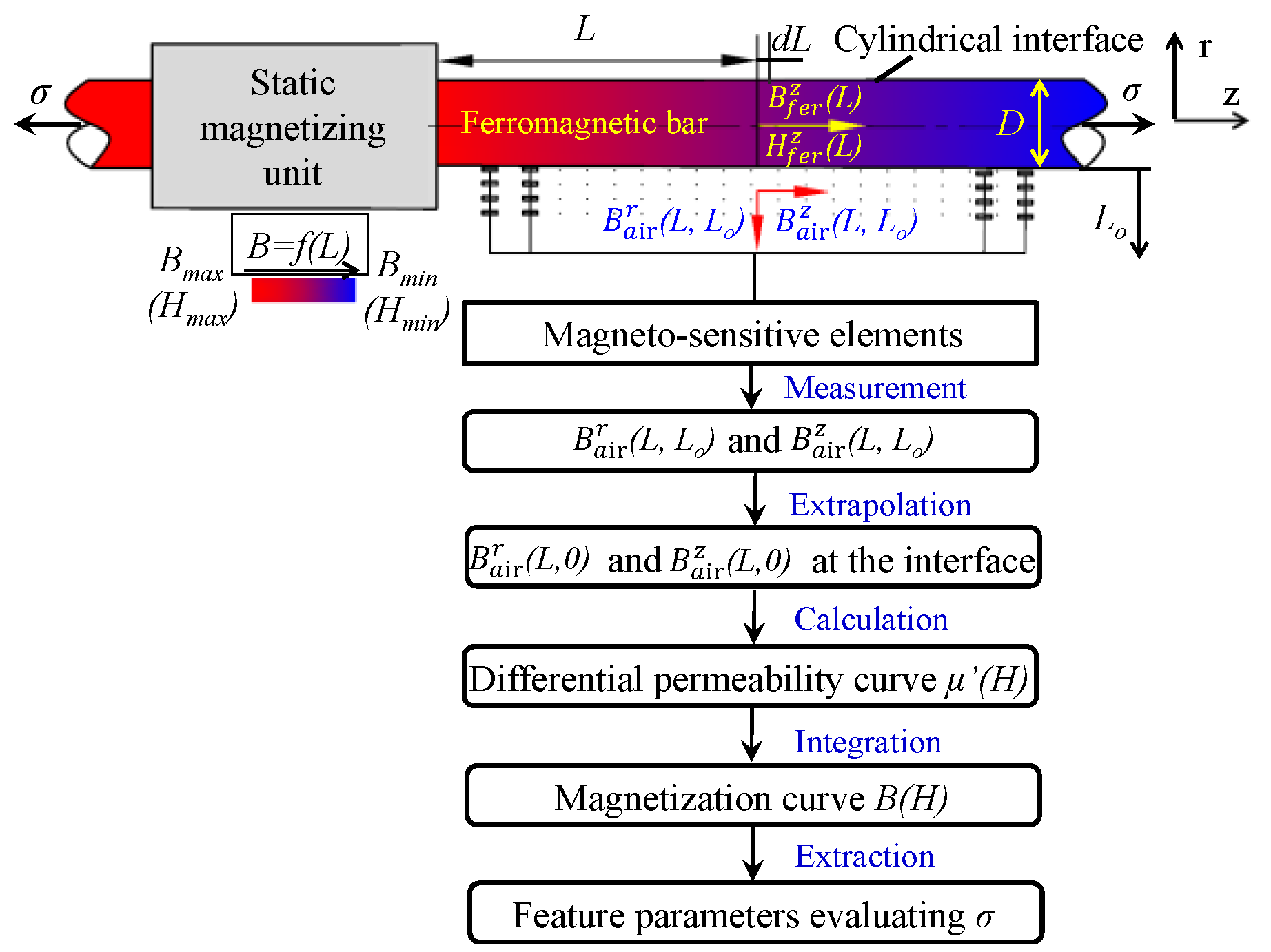
2. The Principle
3. The Development of the Proposed Sensor
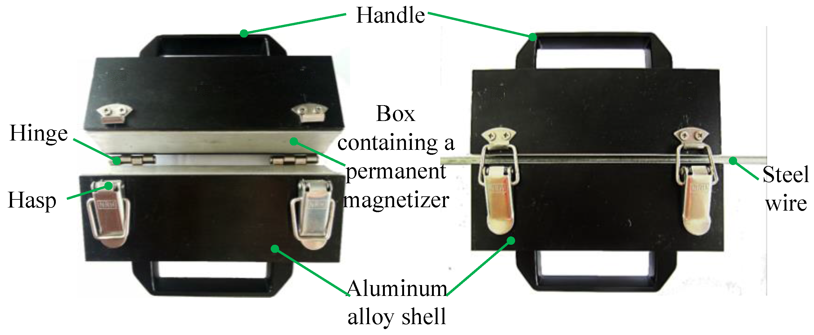
3.1. Static Magnetization Unit
3.2. Magnetic Field Measurement Unit
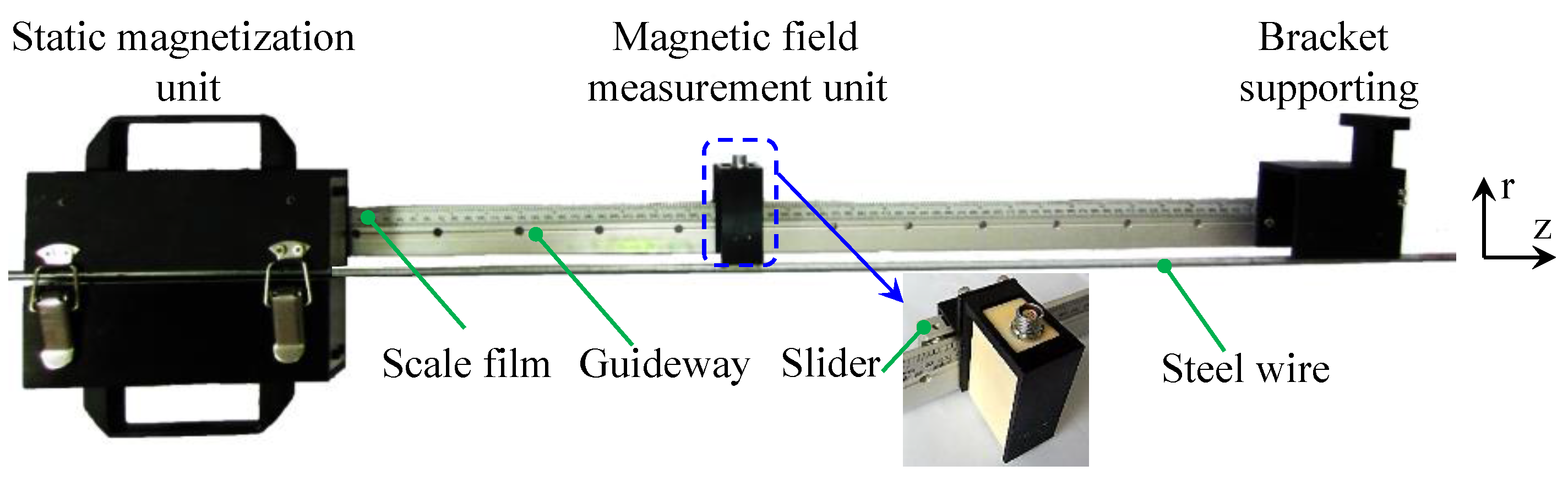
3.3. The Assembly of the Proposed Sensor
4. Experimental Investigation of the Proposed Sensor
4.1. Specimen Preparation
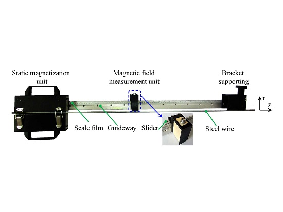
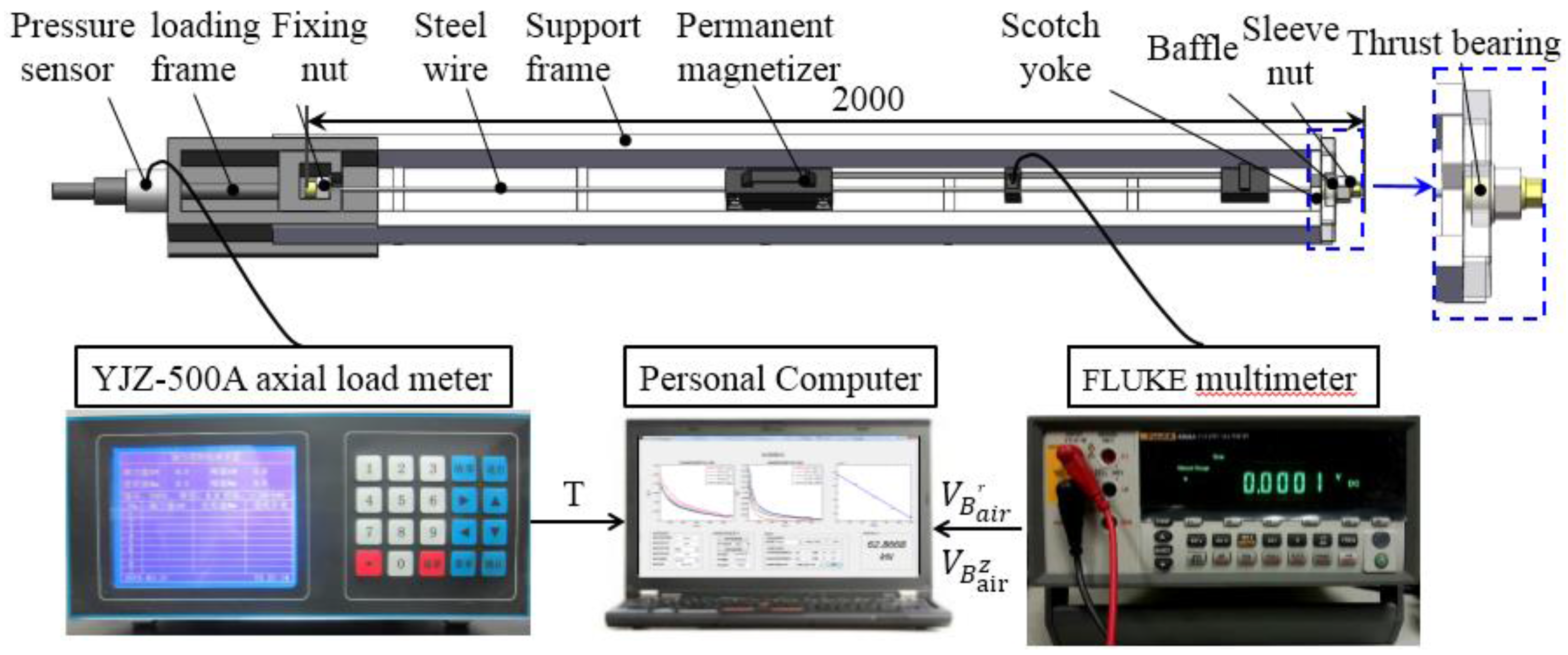
4.2. The Experimental Setup
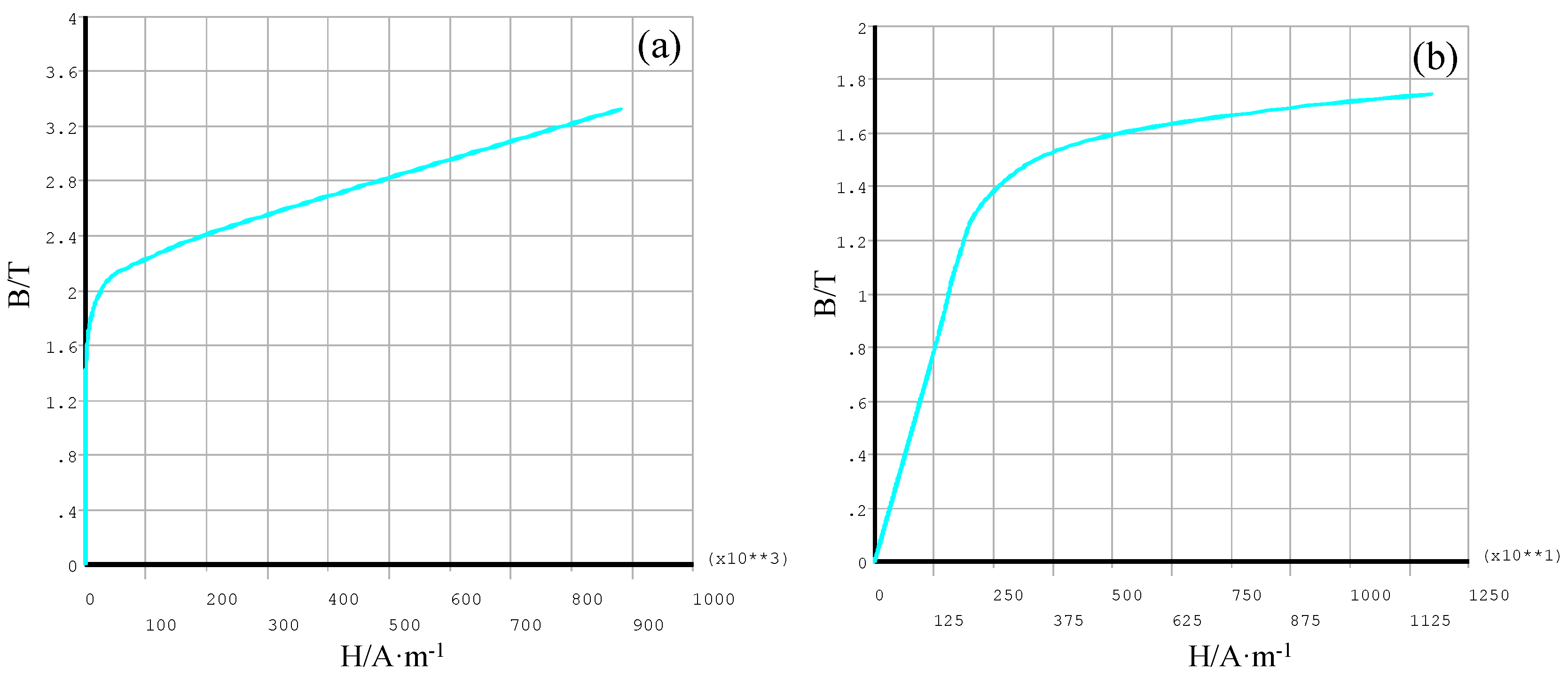
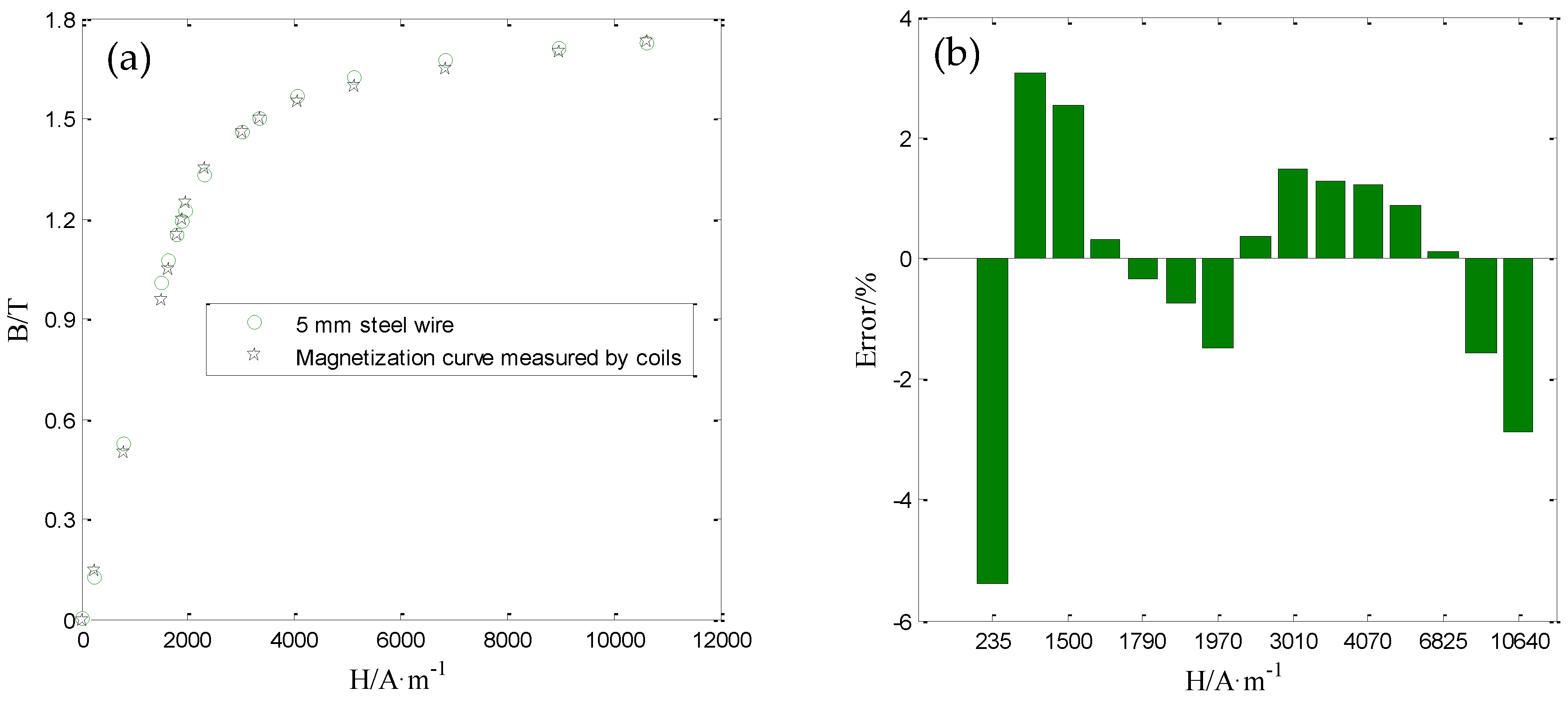
4.3. Measurement Accuracy of the Sensor for Magnetization Curve
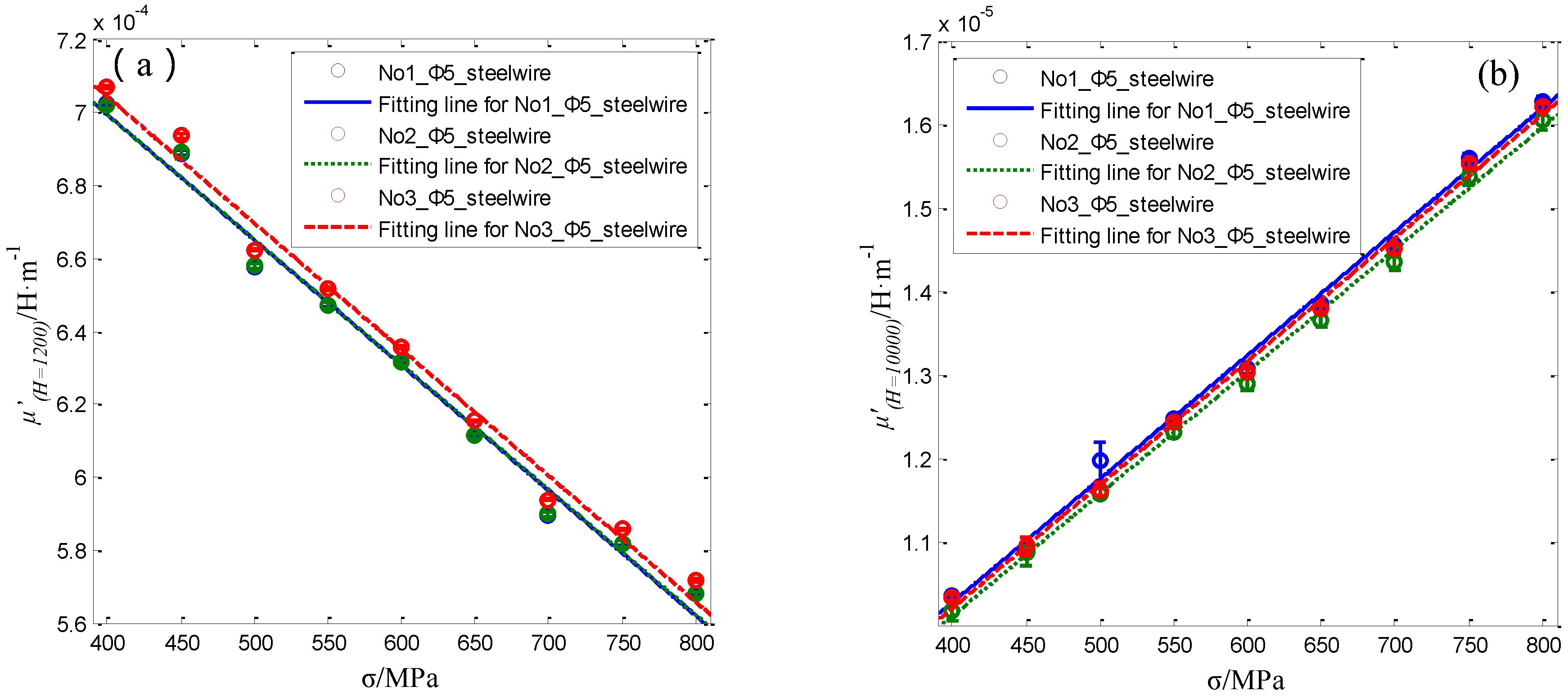
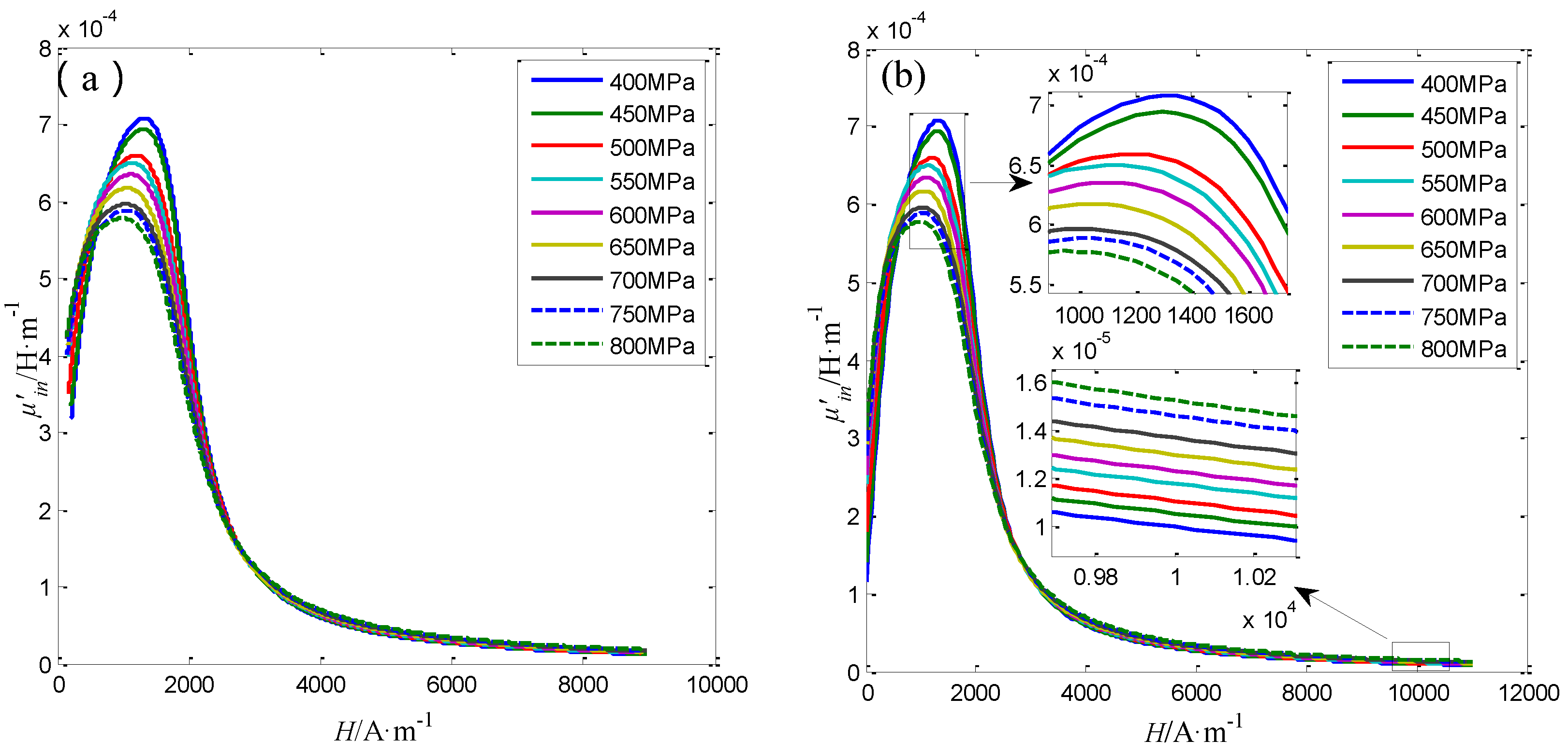
4.4. The Performance of the Sensor for Steel Wires with 5 mm in Diameter
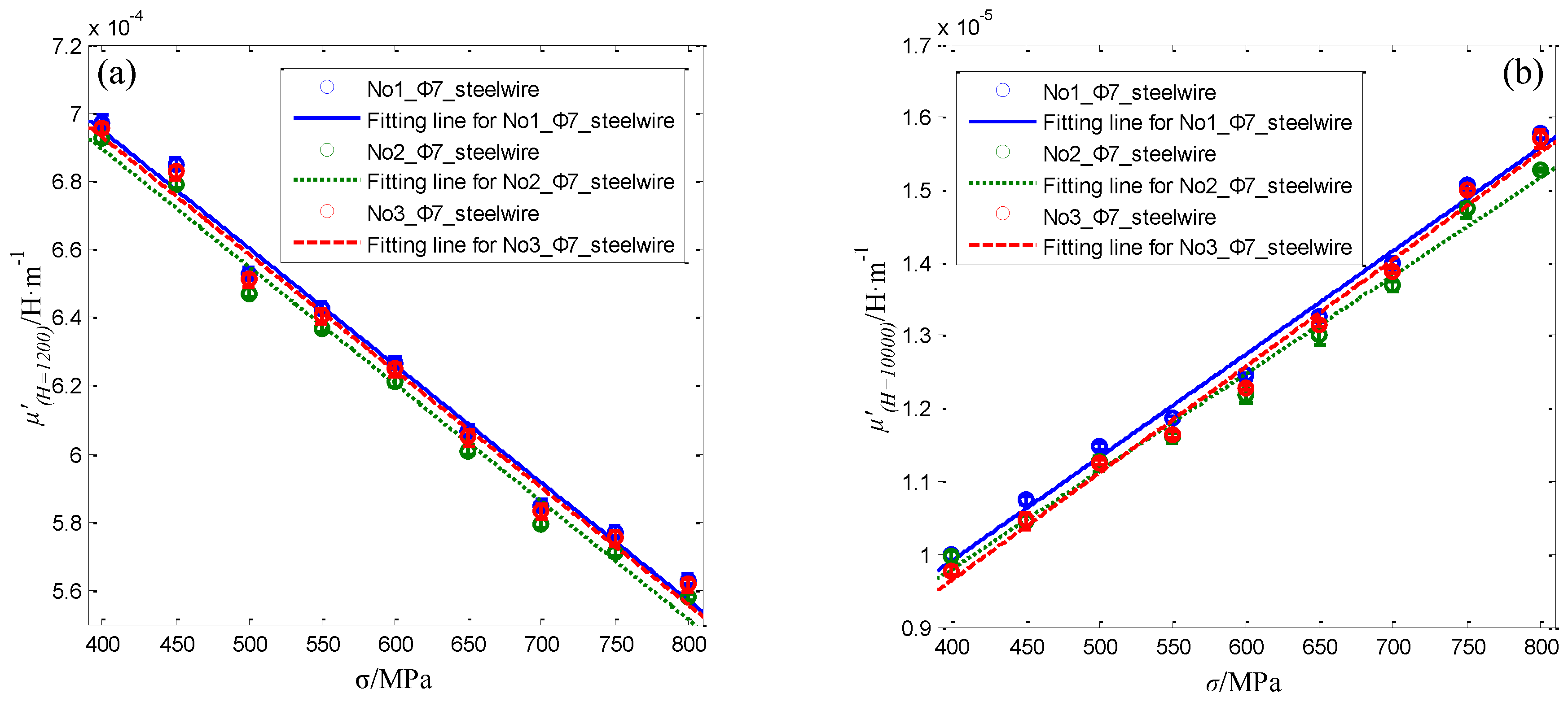
4.5. The Performance of the Sensor for Steel Wires with 7 mm in Diameter
5. Conclusions
Acknowledgments
Author Contributions
Conflicts of Interest
References
- Bozorth, R.M. Ferromagnetism; IEEE Press: Piscataway, NJ, USA, 1993; pp. 595–596. [Google Scholar]
- Wilson, J.W.; Tian, G.Y.; Barrans, S. Residual magnetic field sensing for stress measurement. Sens. Actuators A Phys. 2007, 135, 381–387. [Google Scholar] [CrossRef]
- Gontarz, S.; Radkowski, S. Impact of various factors on relationships between stress and eigen magnetic field in a steel specimen. IEEE. Trans. Magn. 2012, 48, 1143–1154. [Google Scholar] [CrossRef]
- Zhang, R.; Duan, Y.; Or, S.W.; Zhao, Y. Smart Elasto-Magneto-Electric (EME) Sensors for Stress Monitoring of Steel Cables: Design Theory and Experimental Validation. Sensors 2014, 14, 13644–13660. [Google Scholar] [CrossRef] [PubMed]
- Dong, L.H.; Xu, B.S.; Dong, S.Y.; Chen, Q.Z.; Wang, Y.Y.; Zhang, L.; Wang, D.; Yin, D.W. Metal magnetic memory testing for early damage assessment in ferromagnetic materials. J. Cent. South Univ. Technol. 2005, 12, 102–106. [Google Scholar] [CrossRef]
- Tsukada, K.; Furukawa, I.; Kido, T.; Oikawa, M. Tension Measurement Apparatus. US 8890516 B2, 18 November 2014. [Google Scholar]
- Zhang, R. Stress Monitoring for In-service Steel Structures Based on Elasto-Magnetic Effect and Magneto-electric Laminated Composites. Ph.D. Thesis, Zheiiang University, Hangzhou, China, June 2014. [Google Scholar]
- García-Martín, J.; Gómez-Gil, J.; Vázquez-Sánchez, E. Non-destructive techniques based on eddy current testing. Sensors 2011, 11, 2525–2565. [Google Scholar] [CrossRef] [PubMed]
- Dahia, A.; Berthelot, E.; Le Bihan, Y.; Daniel, L. A model-based method for the characterisation of stress in magnetic materials using eddy current non-destructive evaluation. J. Phys. D Appl. Phys. 2015, 48, 195002. [Google Scholar] [CrossRef]
- Schoenekess, H.; Ricken, W.; Becker, W. Method to determine tensile stress alterations in prestressing steel strands by means of an eddy-current technique. IEEE Sens. J. 2007, 7, 1200–1205. [Google Scholar] [CrossRef]
- Kim, J.; Lee, J.; Sohn, H. Detection of tensile force relaxation through eddy current measurement of a pre-stressing strand. In Proceedings of the 2015 World Congress on Advances in Structural Engineering and Mechanics, Incheon, Korea, 25–29 August 2015.
- Wang, G.D. The Application of Magnetoelasticity in Stress Monitoring. Ph.D. Thesis, University of Illinois at Chicago, Chicago, IL, USA, January 2006. [Google Scholar]
- Jarosevic, A. Magnetoelastic method of stress measurement in steel. Smart Struct./NATO Sci. Ser. 1998, 35, 107–114. [Google Scholar]
- Sumitro, S.; Kurokawa, S.; Shimano, K.; Wang, M.L. Monitoring based maintenance utilizing actual stress sensory technology. Smart Mater. Struct. 2005, 14, S68–S78. [Google Scholar] [CrossRef]
- Chen, W.; Liu, L.; Zhang, P.; Hu, S. Non-destructive measurement of the steel cable stress based on magneto-mechanical effect. In Proceedings of the SPIE 7650, Health Monitoring of Structural and Biological Systems 2010, San Diego, CA, USA, 7 March 2010.
- Cho, S.; Yim, J.; Shin, S.W.; Jung, H.; Yun, C.; Wang, M.L. Comparative Field Study of Cable Tension Measurement for a Cable-Stayed Bridge. J. Bridge Eng. 2012, 18, 748–757. [Google Scholar] [CrossRef]
- Zhao, Y.; Wang, M.L. Fast EM stress sensors for large steel cables. In Proceedings of the SPIE 6934, Nondestructive Characterization for Composite Materials, Aerospace Engineering, Civil Infrastructure, and Homeland Security 2008, San Diego, CA, USA, 9 March 2008.
- Wang, G.D.; Wang, M.L.; Zhao, Y.; Chen, Y.; Sun, B.N. Application of EM stress sensors in large steel cables. In Proceedings of SPIE SN09 Conference on Sensors and Smart Structures Technologies for Civil, Mechanical, and Aerospace Systems, San Diego, CA, USA, 6–10 March 2005; pp. 395–406.
- Tang, D.; Huang, S.; Chen, W.; Jiang, J. Study of a steel strand tension sensor with difference single bypass excitation structure based on the magneto-elastic effect. Smart Mater. Struct. 2008, 17, 025019. [Google Scholar] [CrossRef]
- Duan, Y.F.; Zhang, R.; Zhao, Y.; Or, S.W.; Fan, K.Q.; Tang, Z.F. Steel stress monitoring sensors based on elasto-magnetic effect and using magneto-electric laminated composites. J. Appl. Phys. 2012, 111, 07E516. [Google Scholar] [CrossRef]
- Duan, Y.F.; Zhang, R.; Zhao, Y.; Or, S.W.; Fan, K.Q.; Tang, Z.F. Smart elasto-magneto-electric (EME) sensors for stress monitoring of steel structures in railway infrastructures. J. Zhejiang Univ. Sci. A 2011, 12, 895–901. [Google Scholar] [CrossRef]
- Duan, Y.; Zhang, R.; Dong, C.; Luo, Y.; Or, S.W.; Zhao, Y.; Fan, K. Development of Elasto-Magneto-Electric (EME) Sensor for In-Service Cable Force Monitoring. Int. J. Struct. Stab. Dy. 2015, 16, 1640016. [Google Scholar] [CrossRef]
- Deng, D.G.; Wu, X.J. A calculation method for initial magnetization curve under constant magnetization based on time-space transformation. Acta Phys. Sin. 2015, 64, 237503. [Google Scholar]
- Deng, D.G.; Wu, X.J.; Zuo, S. Measurement of initial magnetization curve based on constant magnetic field excited by permanent magnet. Acta Phys. Sin. 2016, 65, 148101. [Google Scholar]
- Bozorth, R.M. Ferromagnetism; IEEE Press: Piscataway, NJ, USA, 1993; pp. 476–477. [Google Scholar]
- Chikazumi, S. Physics of Ferromagnetism, 2nd ed.; Oxford University Press: Oxford, UK, 1997; pp. 503–508. [Google Scholar]
- Gimmel, B.; Feller, U. Modeling of magnetic and magnetoelastic behavior of prestressing steel near saturation. IEEE. Trans. Magn. 1995, 31, 2241–2248. [Google Scholar] [CrossRef]
- Garshelis, I.J.; Tollens, S.P.; Kari, R.J.; Vandenbossche, L.P.; Dupré, L.R. Drag force measurement: A means for determining hysteresis loss. J. Appl. Phys. 2006, 99, 08D910. [Google Scholar] [CrossRef]
- Xu, J.; Wu, X.; Cheng, C.; Ben, A. A magnetic flux leakage and magnetostrictive guided wave hybrid transducer for detecting bridge cables. Sensors 2012, 12, 518–533. [Google Scholar] [CrossRef] [PubMed]
- Wang, J.; She, S.; Zhang, S. An improved Helmholtz coil and analysis of its magnetic field homogeneity. Rev. Sci. Instrum. 2002, 73, 2175–2179. [Google Scholar] [CrossRef]
- Stupakov, O. Investigation of applicability of extrapolation method for sample field determination in single-yoke measuring setup. J. Magn. Magn. Mater. 2006, 307, 279–287. [Google Scholar] [CrossRef]
- Perevertov, O. Measurement of the surface field on open magnetic samples by the extrapolation method. Rev. Sci. Instrum. 2005, 76, 104701. [Google Scholar] [CrossRef]
- Hovorka, O.; Lloyd, G.M.; Wang, M.L. Comparison of surface H-field measurements using Hall sensors and a novel multiple sense coil approach. In Proceedings of the IEEE Sensors, First IEEE International Conference on Sensors, Orlando, FL, USA, 12–14 June 2002.
- Wang, M.L.; Lloyd, G.M.; Hovorka, O. Development of a remote coil magneto-elastic stress sensor for steel cables. In Proceedings of the SPIE 4337, 6th Annual International Symposium on NDE for Health Monitoring and Diagnostics, Newport Beach, CA, USA, 3 August 2001; pp. 122–128.


| C | Si | Mn | P | S | Ni | Cr | Cu |
|---|---|---|---|---|---|---|---|
| 0.81 | 0.22 | 0.82 | 0.013 | 0.014 | 0.01 | 0.26 | 0.01 |
| Working Region | Rayleigh Region | Region Approach to Saturation |
|---|---|---|
| (H1, μ’in1)/(A/m, × 10−4 H/m)) | (141.5, 5.404) | (8906.9, 0.1088) |
| (H2, μ’in2)/(A/m, × 10−4 H/m)) | (143.0, 5.424) | (8944.7, 0.1073) |
| Specimen Number | Feature Parameters | Fitting Equation | R2 |
|---|---|---|---|
| No.1 | μ’(H = 1200) | μ’(H = 1200) = −3.4345 × 10⁻⁷ σ + 8.3691 × 10⁻⁴ | 0.9890 |
| μ’(H = 10000) | μ’(H = 10000) = 1.4798 × 10⁻⁸ σ + 4.3456 × 10⁻⁶ | 0.9948 | |
| No.2 | μ’(H = 1200) | μ’(H = 1200) = −3.4298 × 10⁻⁷ σ + 8.3679 × 10⁻⁴ | 0.9891 |
| μ’(H = 10000) | μ’(H = 10000) = 1.4626 × 10⁻⁸ σ + 4.2536 × 10⁻⁶ | 0.9974 | |
| No.3 | μ’(H = 1200) | μ’(H = 1200) = −3.4626 × 10⁻⁷ σ + 8.4293 × 10⁻⁴ | 0.9892 |
| μ’(H = 10000) | μ’(H = 10000) = 1.4773 × 10⁻⁸ σ + 4.2894 × 10⁻⁶ | 0.9970 |
| Specimen Number | Feature Parameters | Fitting Equation | R2 |
|---|---|---|---|
| No.1 | μ’(H = 1200) | μ’(H = 1200) = −3.4404 × 10⁻⁷ σ + 8.325 × 10⁻⁴ | 0.9886 |
| μ’(H = 10000) | μ’(H = 10000) = 1.4179 × 10⁻⁸ σ + 4.232 × 10⁻⁶ | 0.9902 | |
| No.2 | μ’(H = 1200) | μ’(H = 1200) = −3.446 × 10⁻⁷ σ + 8.2729 × 10⁻⁴ | 0.9879 |
| μ’(H = 10000) | μ’(H = 10000) = 1.3432 × 10⁻⁸ σ + 4.4126 × 10⁻⁶ | 0.9896 | |
| No.3 | μ’(H = 1200) | μ’(H = 1200) = −3.4241 × 10⁻⁷ σ + 8.2994 × 10⁻⁴ | 0.9885 |
| μ’(H = 10000) | μ’(H = 10000) = 1.468 × 10⁻⁸ σ + 3.7638 × 10⁻⁶ | 0.9904 |
© 2016 by the authors; licensee MDPI, Basel, Switzerland. This article is an open access article distributed under the terms and conditions of the Creative Commons Attribution (CC-BY) license (http://creativecommons.org/licenses/by/4.0/).
Share and Cite
Deng, D.; Wu, X.; Zuo, S. A Steel Wire Stress Measuring Sensor Based on the Static Magnetization by Permanent Magnets. Sensors 2016, 16, 1650. https://doi.org/10.3390/s16101650
Deng D, Wu X, Zuo S. A Steel Wire Stress Measuring Sensor Based on the Static Magnetization by Permanent Magnets. Sensors. 2016; 16(10):1650. https://doi.org/10.3390/s16101650
Chicago/Turabian StyleDeng, Dongge, Xinjun Wu, and Su Zuo. 2016. "A Steel Wire Stress Measuring Sensor Based on the Static Magnetization by Permanent Magnets" Sensors 16, no. 10: 1650. https://doi.org/10.3390/s16101650
APA StyleDeng, D., Wu, X., & Zuo, S. (2016). A Steel Wire Stress Measuring Sensor Based on the Static Magnetization by Permanent Magnets. Sensors, 16(10), 1650. https://doi.org/10.3390/s16101650