
Analysis on Target Detection and Classification in LTE Based Passive Forward Scattering Radar

Abstract
:1. Introduction
2. Target Detection in Passive Forward Scattering Radar
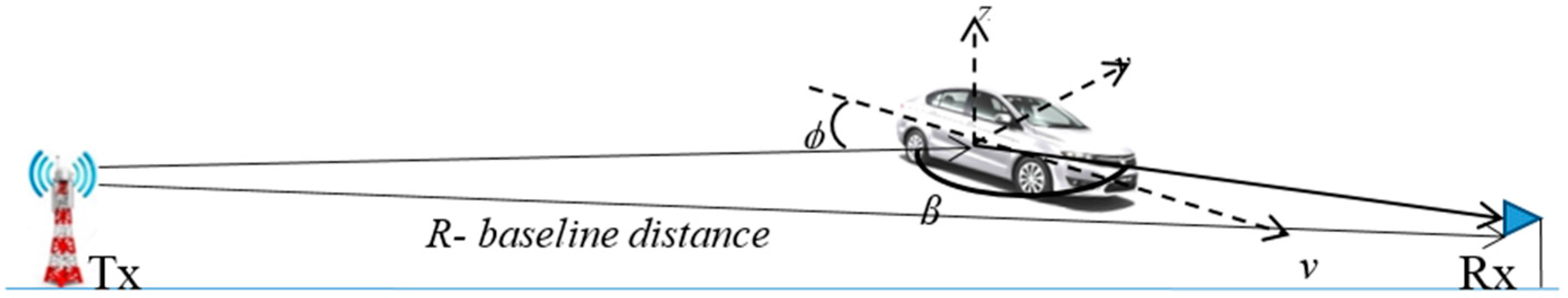
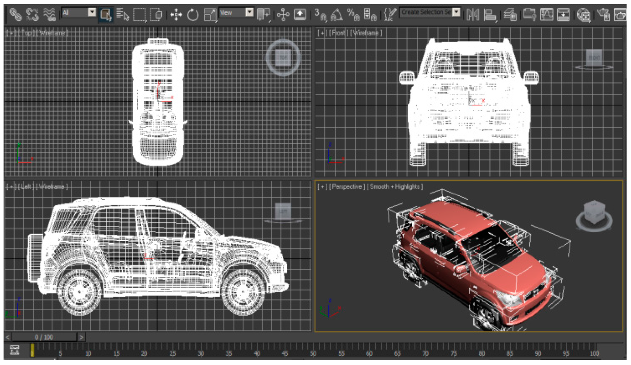
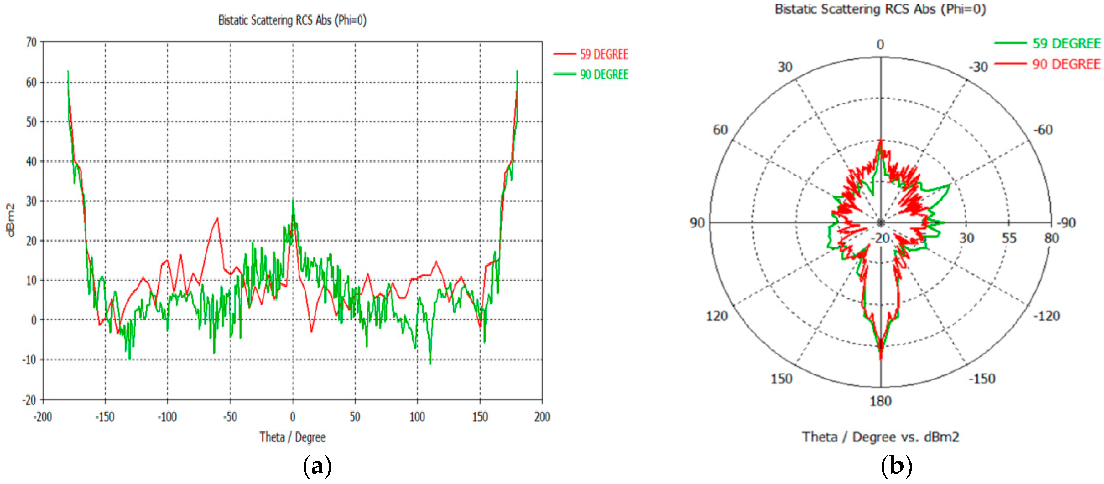
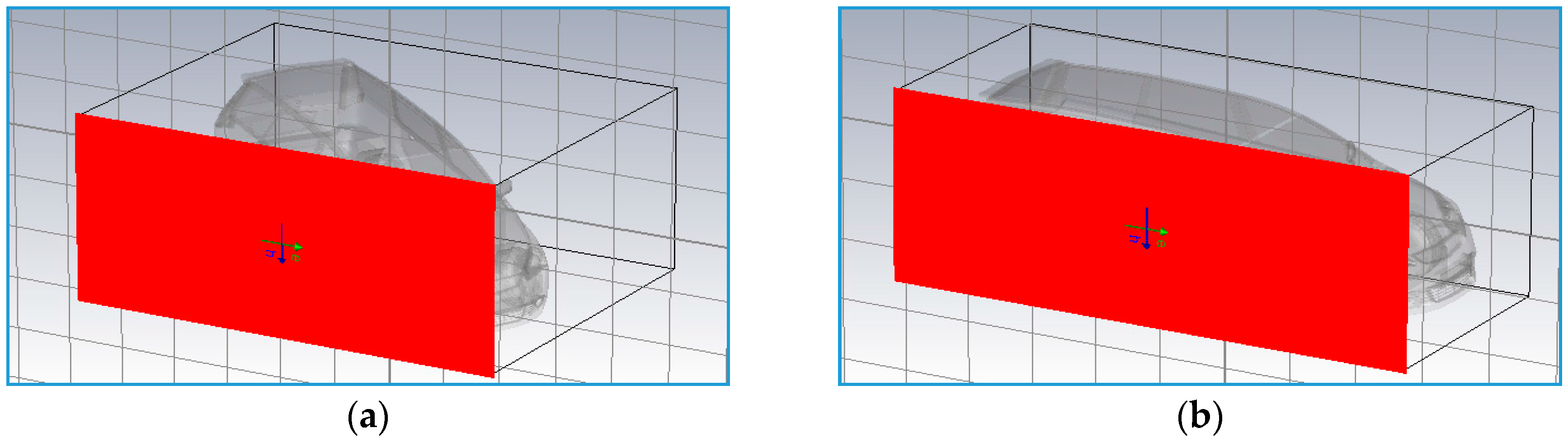
2.1. Passive Forward Scatter Radar Cross Section
2.2. Target Doppler Signature in Passive FSR
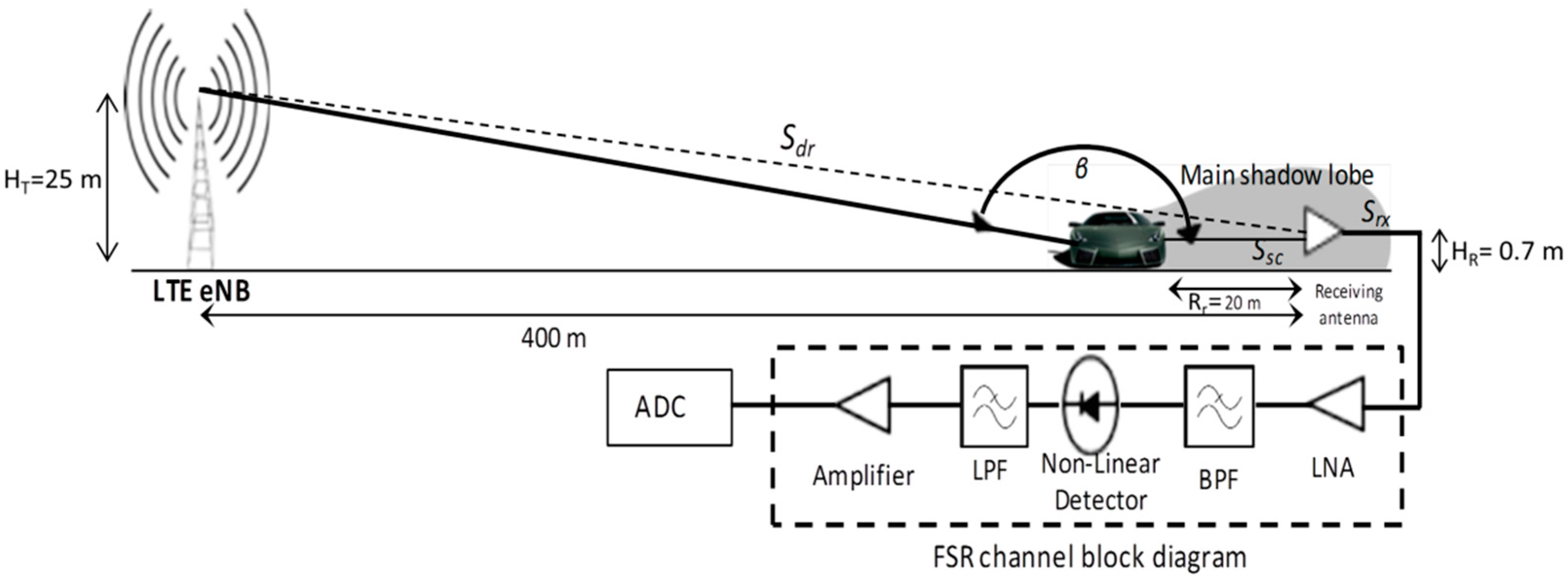
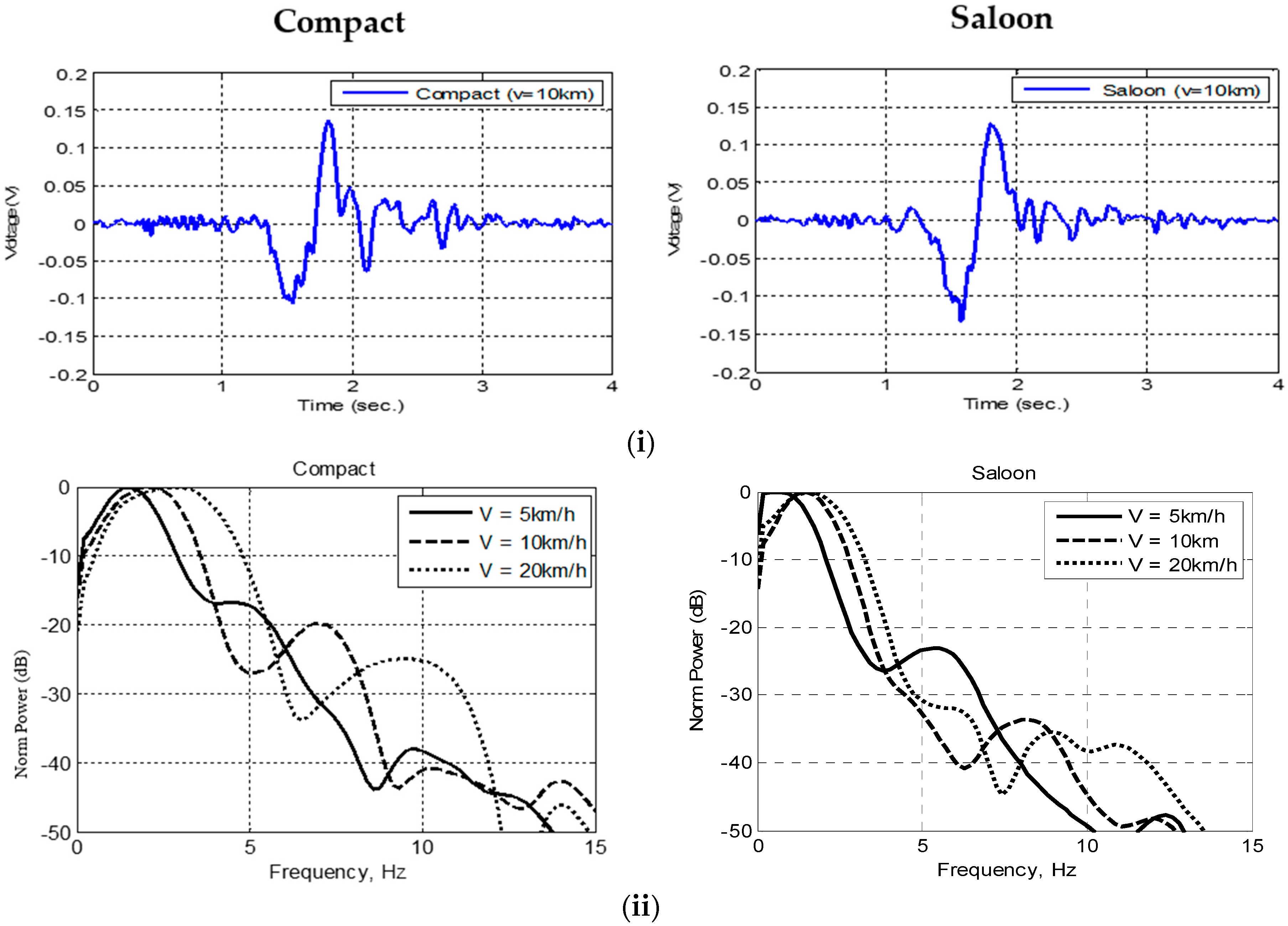
2.3. Received Signal and Target’s Features in Passive FSR
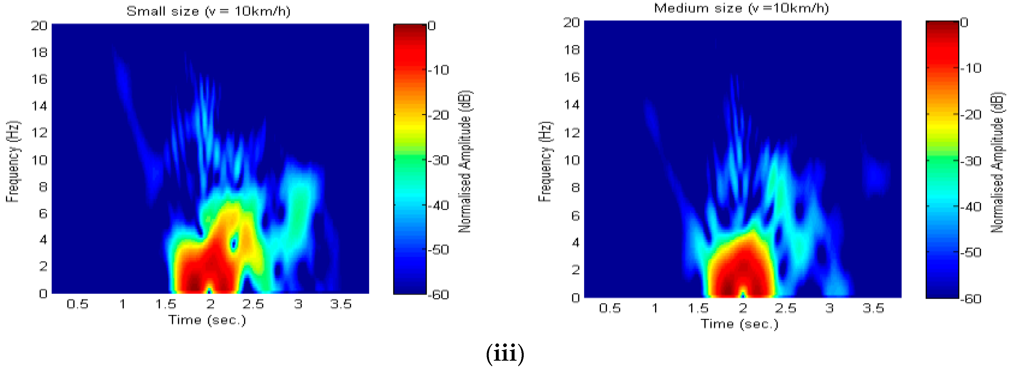
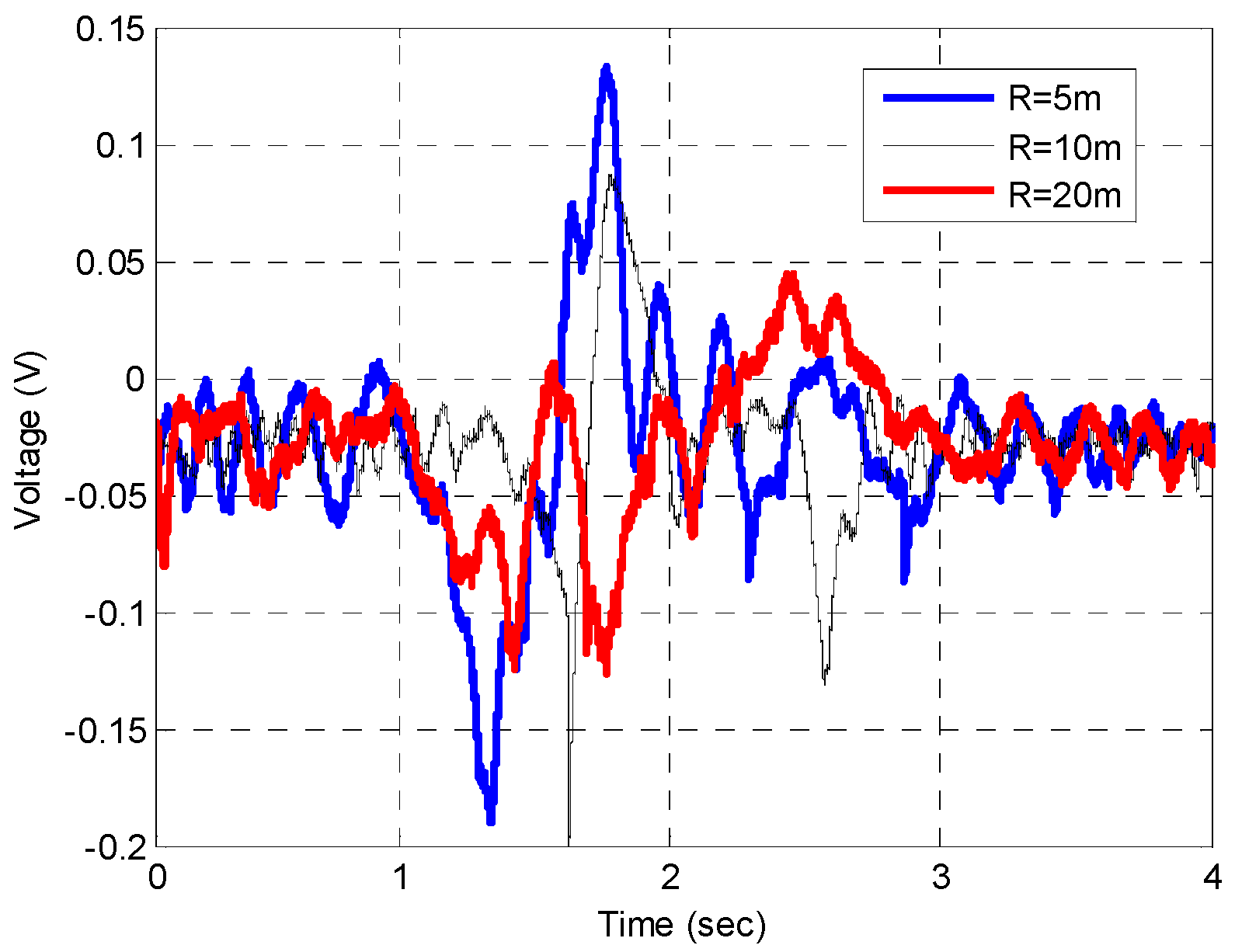
- the amplitudes of Doppler signatures to the target’s forward scatter cross section, hence, the Saloon car had a bigger forward scatter cross section, which was reflected in the amplitudes of their signature,
- the signal span in time domain to the length of the target, hence, the Saloon car also had a longer body, which was reflected in the signal span of the forward scatter main lobe.
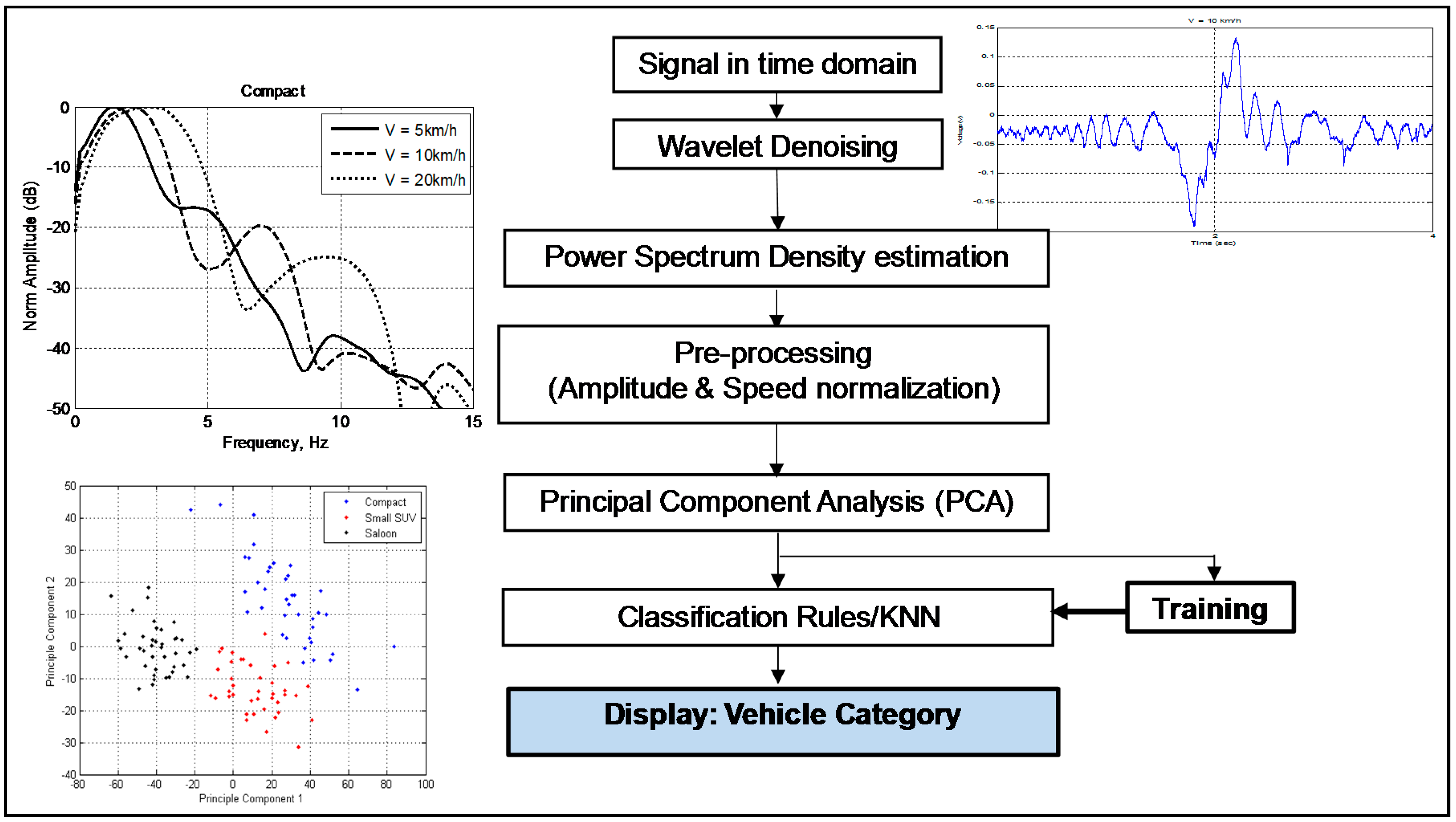
3. Target Classification in Passive Forward Scattering Radar
3.1. Evaluation of Target’s Baseline Crossing
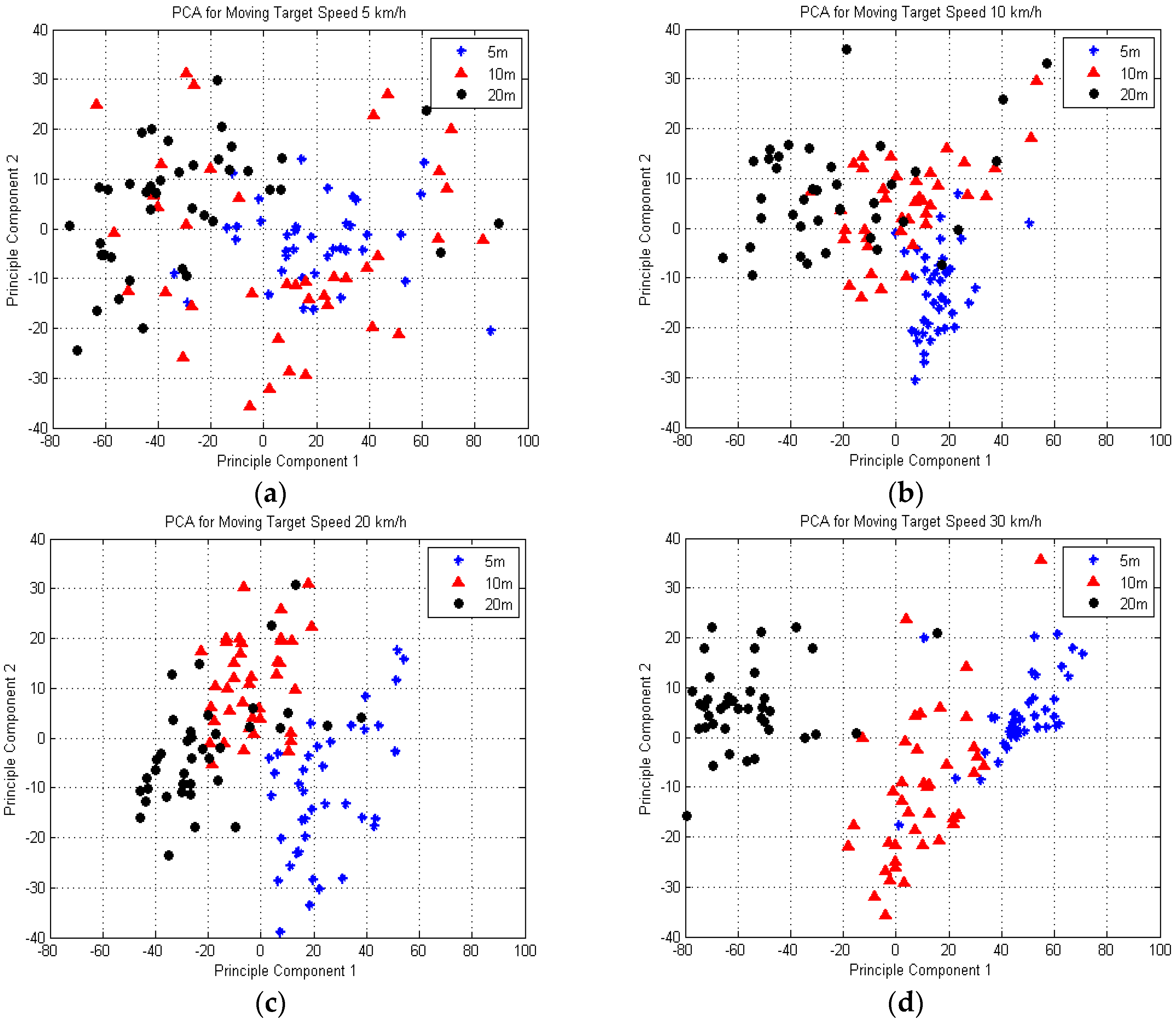
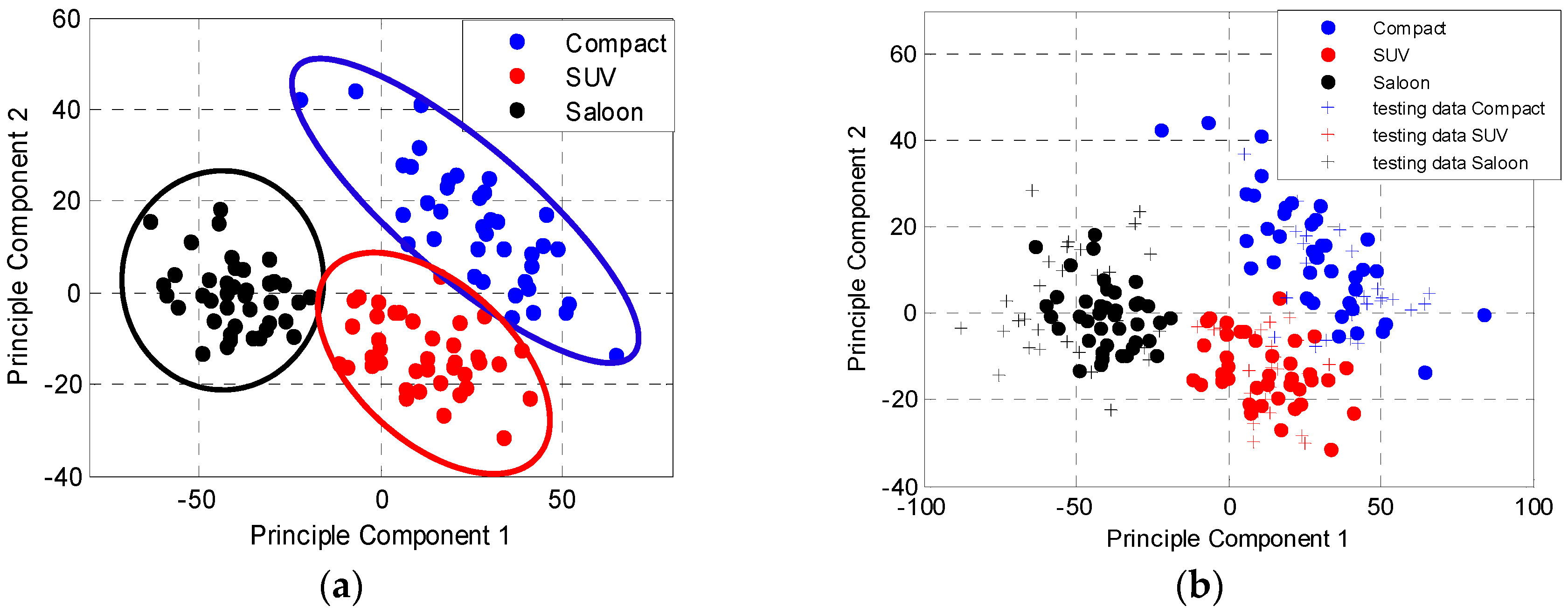
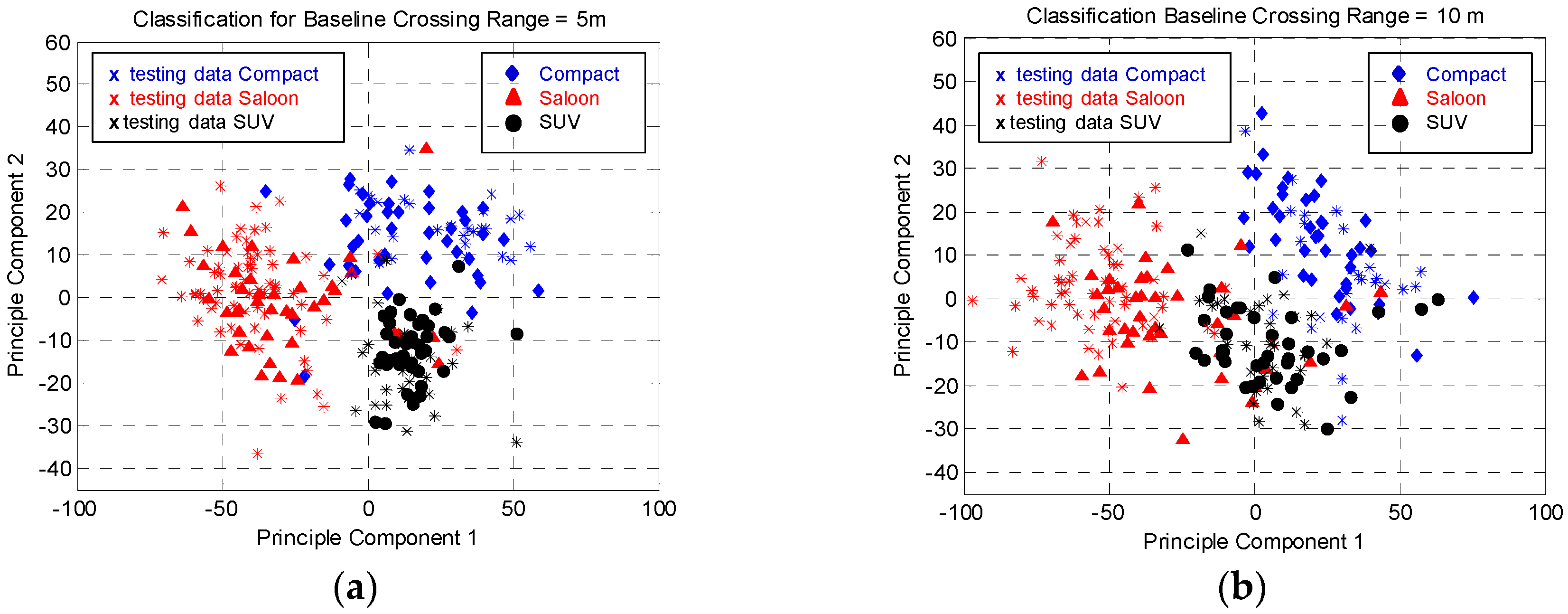
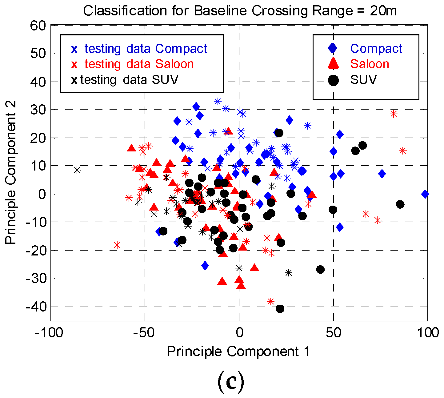
3.2. Vehicle Classification Performance at Different Baseline Crossing Range
4. Conclusions
Author Contributions
Conflicts of Interest
Abbreviations
| FSR | Forward Scattering Radar |
| RCS | Radar Cross Section |
| LTE | Long-Term Evolution |
| AF | Ambiguity Function |
| FSML | Forward Scatter Main Lobe |
| FS | Forward Scatter |
| GSM | Global Systems for Mobile |
| SUV | Sport Utility Vehicle |
| CST | Computer Simulation Technology |
| ADC | Analogue to Digital Converter |
| PCA | Principle Components Analysis |
| FFT | Fast Fourier Transform |
| PC | Principle Component |
References
- Cherniakov, M. Bistatic Radar: Emerging Technology; John Wiley and Sons, Ltd.: Chichester, UK, 2008. [Google Scholar]
- Cherniakov, M.; Abdullah, R.S.A.R.; Jancovic, P.; Salous, M.; Chapursky, V. Automatic ground target classification using forward scattering radar. IEE Proc. Radar Sonar Navig. 2006, 153, 427–437. [Google Scholar] [CrossRef]
- Marra, M.; De Luca, A.; Hristov, S.; Daniel, L.; Gashinova, M.; Cherniakov, M. New algorithm for signal detection in passive FSR. In Proceedings of the 2015 IEEE Radar Conference, Johannesburg, South Africa, 27–30 October 2015; pp. 218–223.
- Pastina, D.; Contu, M.; Lombardo, P.; Gashinova, M.; De Luca, A.; Daniel, L.; Cherniakov, M. Target motion estimation via multi-node forward scatter radar system. IET Radar Sonar Navig. 2016, 10, 1. [Google Scholar] [CrossRef]
- Griffiths, H.D.; Long, N.R.W. Television-based bistatic radar. IEE Proc. F Commun. Radar Signal Process. 1986, 133, 649–657. [Google Scholar] [CrossRef]
- Howland, P.E.; Maksimiuk, D.; Reitsma, G. FM radio based bistatic radar. IEE Proc. Radar Sonar Navig. 2005, 152, 107–115. [Google Scholar] [CrossRef]
- Poullin, D. Passive detection using digital broadcasters (DAB, DVB) with COFDM modulation. IEE Proc. Radar Sonar Navig. 2005, 152, 143–152. [Google Scholar] [CrossRef]
- Bárcena-Humanes, J.L.; Gómez-Hoyo, P.J.; Jarabo-Amores, M.P.; Mata-Moya, D.; Del-Rey-Maestre, N. Feasibility study of EO SARs as opportunity illuminators in passive radars: PAZ-based case study. Sensors 2015, 15, 29079–29106. [Google Scholar] [CrossRef] [PubMed]
- Griffiths, H.D.; Garnett, A.J.; Baker, C.J.; Keaveney, S. Bistatic radar using satellite-borne illuminators of opportunity. In Proceedings of the Radar International Conference, Brighton, UK, 12–13 October 1992; pp. 276–279.
- Hongbo, S.; Tan, D.K.P.; Lu, Y. Aircraft target measurements using A GSM-based passive radar. In Proceedings of the 2008 IEEE Radar Conference, Rome, Italy, 26–30 May 2008; pp. 1–6.
- Raja Abdullah, R.S.A.; Salah, A.A.; Ismail, A.; Hashim, F.H.; Abdul Rashid, N.E.; Abdul Aziz, N.H. Experimental investigation on target detection and tracking in passive radar using long-term evolution signal. IET Radar Sonar Navig. 2016, 10, 577–585. [Google Scholar] [CrossRef]
- Raja Abdullah, R.S.A.; Rasid, M.F.A.; Mohamed, M.K.H. Improvement in detection with forward scattering radar. Sci. China Inf. Sci. 2011, 54, 2660–2672. [Google Scholar] [CrossRef]
- Gashinova, M.; Daniel, L.; Hoare, E.; Sizov, V.; Kabakchiev, K.; Cherniakov, M. Signal characterisation and processing in the forward scatter mode of bistatic passive coherent location systems. EURASIP J. Adv. Signal Process. 2013, 2013, 36. [Google Scholar] [CrossRef]
- Suberviola, I.; Mayordome, I.; Mendizabal, J. Experimental results of air target detection with GPS forward scattering radar. IEEE Geosci. Remote Sens. Lett. 2012, 9, 47–51. [Google Scholar] [CrossRef]
- Behar, V.; Kabakchiev, C. Detectability of Air Target Detection using Bistatic Radar Based on GPS L5 Signals. In Proceedings of the 12th International Radar Symposium (IRS), Leipzig, Germany, 7–9 September 2011; pp. 212–217.
- Kabakchiev, C.; Garvanov, I.; Behar, V.; Daskalov, P.; Rohling, H. Study of moving target shadows using passive Forward Scatter radar systems. In Proceedings of the 2014 15th International Radar Symposium (IRS), Gdansk, Poland, 16–18 June 2014; pp. 1–4.
- Krysik, P.; Kulpa, K.; Samczyński, P. GSM based passive receiver using forward scatter radar geometry. In Proceedings of the 2014 15th International Radar Symposium (IRS), Dresden, Germany, 19–21 June 2013; pp. 637–642.
- Salah, A.A.; Abdullah, R.S.A.; Ismail, A.; Hashim, F.; Leow, C.Y.; Roslee, M.B.; Rashid, N.A. Feasibility study of LTE signal as a new illuminators of opportunity for passive radar applications. In Proceedings of the 2013 IEEE International RF and Microwave Conference (RFM), Penang, Malaysia, 9–11 December 2013; pp. 258–262.
- Ahmadi, S. An overview of 3GPP long-term evolution radio access network. In New Directions in Wireless Communications Research; Springer: Hillsboro, TX, USA, 2009; pp. 431–465. [Google Scholar]
- Duda, R.O.; Hart, P.E.; Stork, D.G. Pattern Classification; John Wiley & Sons: New York, NY, USA, 2000; pp. 2–4. [Google Scholar]
- Welch, P.D. The use of fast Fourier transform for the estimation of power spectra: A method based on time averaging over short, modified periodograms. IEEE Trans. Audio Electroacoust. 1967, 15, 70–73. [Google Scholar] [CrossRef]
- Noor Hafizah, A.A.; Haziq Hazwan, M.Y.; Nur Emileen, A.R.; Raja Syamsul Azmir, R.A.; Asem, S. RCS analysis on different targets and bistatic angles using LTE frequency. Int. J. Ind. Electron. Electr. Eng. 2015, 3, 1–4. [Google Scholar]


| Parameters | Incident Angle, φ | |
|---|---|---|
| 59° | 90° | |
| Bistatic angle, β of Max RCS (°) | 180.00 | 180.00 |
| Max RCS magnitude (dBm2) | 60.04 | 62.75 |
| Side lobe level (dB) | −31.30 | −23.50 |
| Category | Compact | Saloon | Small SUV |
|---|---|---|---|
| Actual car used during experiment to represent each category |  |  |  |
| No. of collected data used for classification | 70 | 73 | 70 |
| Vehicle’s Dimension | L = 3395 mm | L = 4360 mm | L = 4420 mm |
| H = 1415 mm | H = 1385 mm | H = 1740 mm |
| Vehicle-Category | NO.V—For Testing | Automatically Classified as (%) | ||
|---|---|---|---|---|
| Compact | Saloon | Small SUV | ||
| Compact | 30 | 92 | 0 | 8 |
| Saloon | 33 | 0 | 100 | 0 |
| Small SUV | 30 | 4 | 0 | 96 |
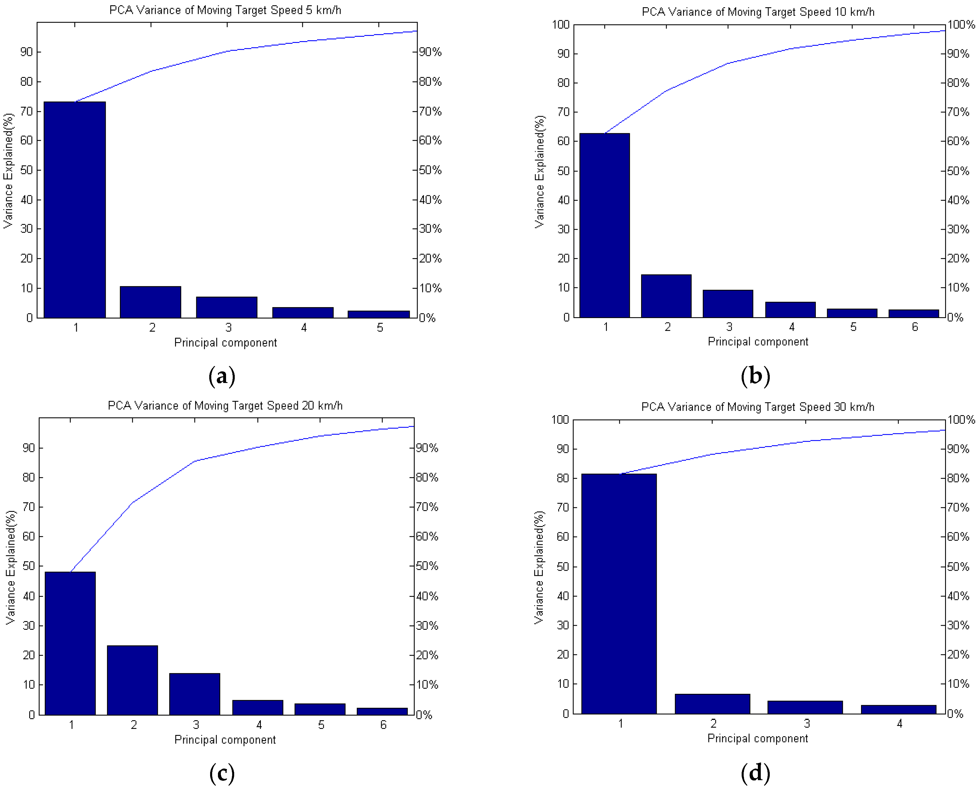
| Target’s Speed (km/h) | 5 | 10 | 20 | 30 |
| Variance Explained (%) | 73 | 63 | 48 | 82 |
| Range, RR (m) | 5 | 10 | 20 | ||||||
|---|---|---|---|---|---|---|---|---|---|
| Type of Vehicle | Compact | Saloon | SUV | Compact | Saloon | SUV | Compact | Saloon | SUV |
| Training Data | 40 | 40 | 40 | 40 | 40 | 40 | 40 | 40 | 40 |
| Testing Data | 30 | 69 | 33 | 27 | 61 | 35 | 32 | 39 | 25 |
| Classification | 30 | 67 | 33 | 21 | 57 | 32 | 30 | 33 | 17 |
| Classification (%) | 100 | 97.1 | 100 | 77.78 | 93.44 | 91.4 | 93.75 | 84.62 | 68.0 |
| Average Classification (%) | 99.0 | 87.54 | 82.12 | ||||||
© 2016 by the authors; licensee MDPI, Basel, Switzerland. This article is an open access article distributed under the terms and conditions of the Creative Commons Attribution (CC-BY) license (http://creativecommons.org/licenses/by/4.0/).
Share and Cite
Raja Abdullah, R.S.A.; Abdul Aziz, N.H.; Abdul Rashid, N.E.; Ahmad Salah, A.; Hashim, F. Analysis on Target Detection and Classification in LTE Based Passive Forward Scattering Radar. Sensors 2016, 16, 1607. https://doi.org/10.3390/s16101607
Raja Abdullah RSA, Abdul Aziz NH, Abdul Rashid NE, Ahmad Salah A, Hashim F. Analysis on Target Detection and Classification in LTE Based Passive Forward Scattering Radar. Sensors. 2016; 16(10):1607. https://doi.org/10.3390/s16101607
Chicago/Turabian StyleRaja Abdullah, Raja Syamsul Azmir, Noor Hafizah Abdul Aziz, Nur Emileen Abdul Rashid, Asem Ahmad Salah, and Fazirulhisyam Hashim. 2016. "Analysis on Target Detection and Classification in LTE Based Passive Forward Scattering Radar" Sensors 16, no. 10: 1607. https://doi.org/10.3390/s16101607
APA StyleRaja Abdullah, R. S. A., Abdul Aziz, N. H., Abdul Rashid, N. E., Ahmad Salah, A., & Hashim, F. (2016). Analysis on Target Detection and Classification in LTE Based Passive Forward Scattering Radar. Sensors, 16(10), 1607. https://doi.org/10.3390/s16101607