
Structured Light-Based 3D Reconstruction System for Plants


Abstract
:1. Introduction
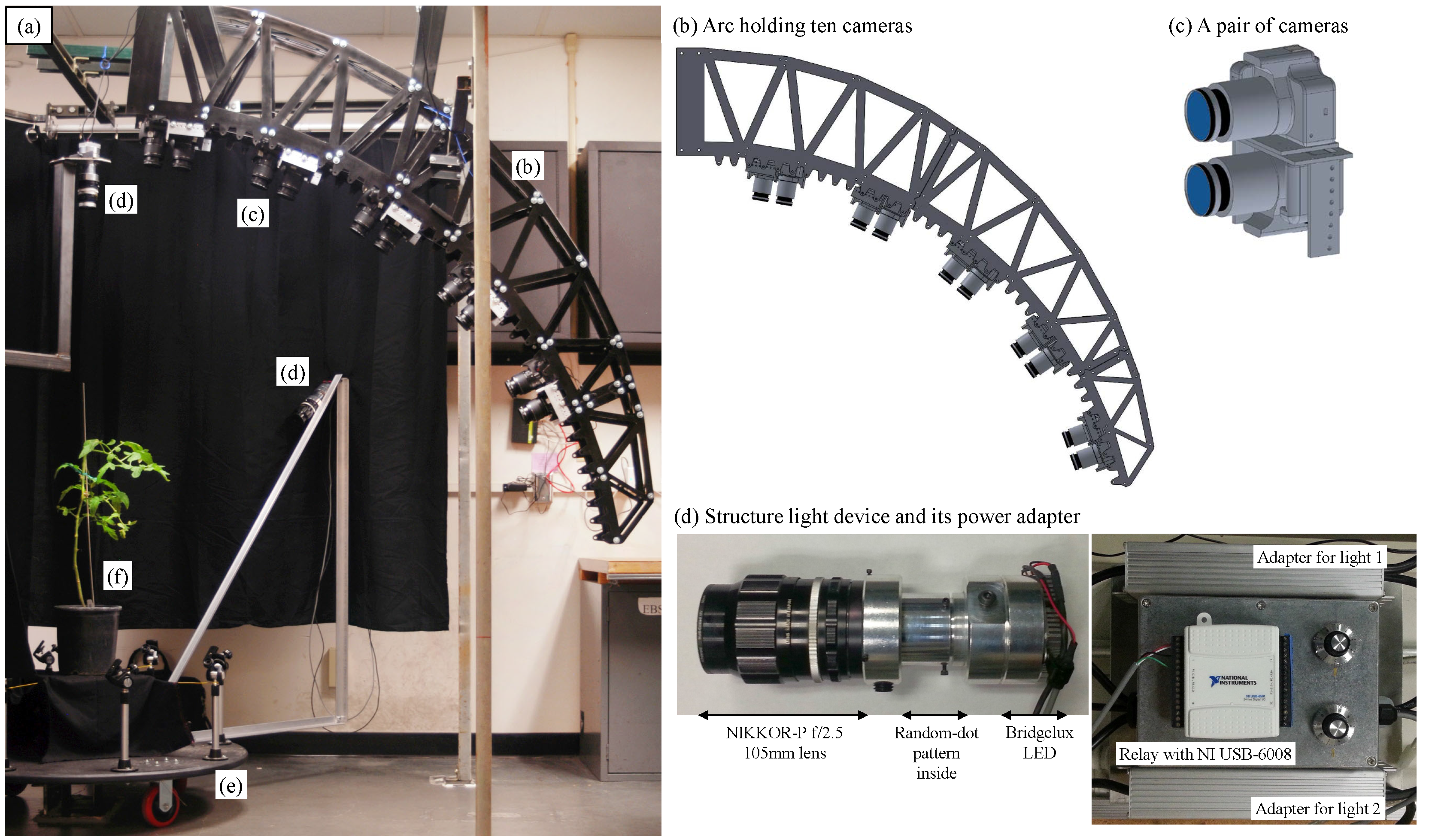
2. System Design

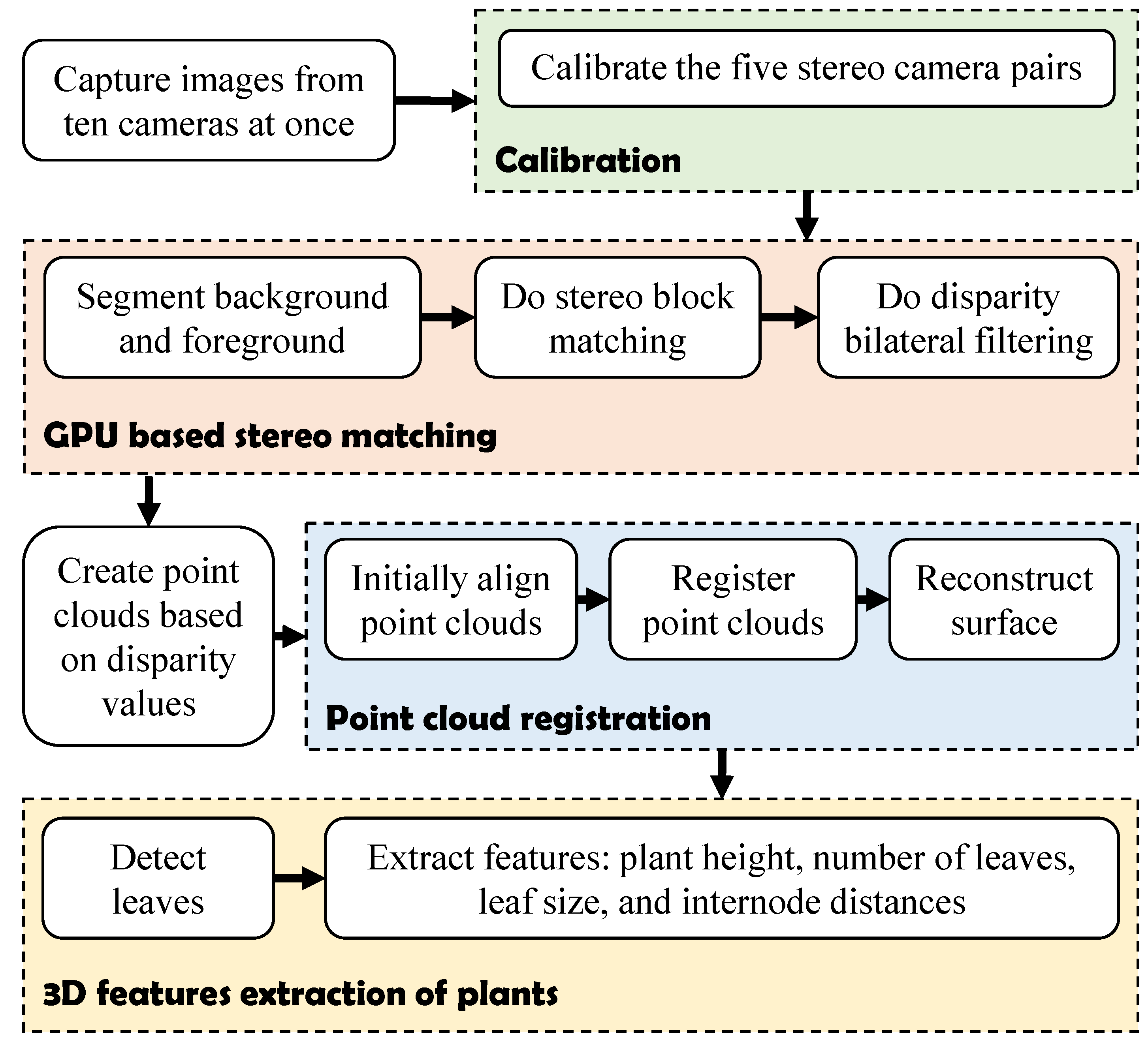
3. Software Algorithms
3.1. Stereo Camera Calibration

3.2. Stereo Matching
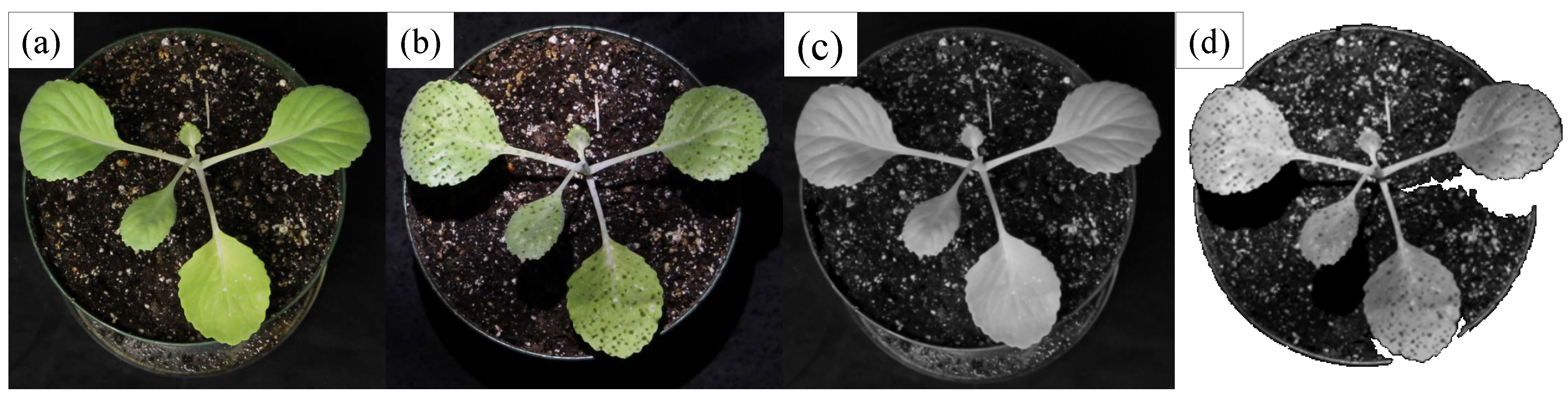
3.2.1. Background and Foreground Segmentation

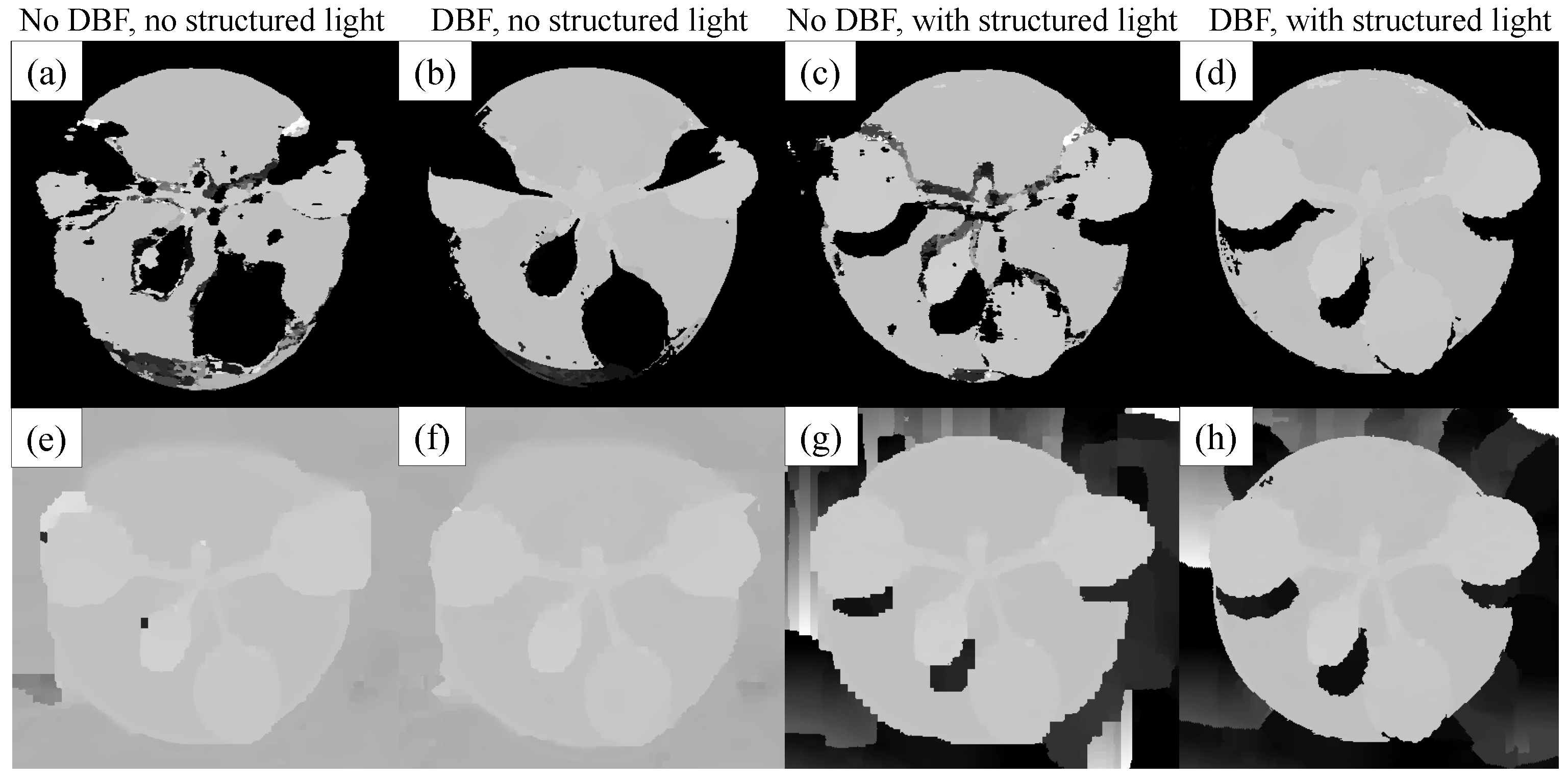
3.2.2. Stereo Block Matching
3.2.3. Disparity Bilateral Filtering

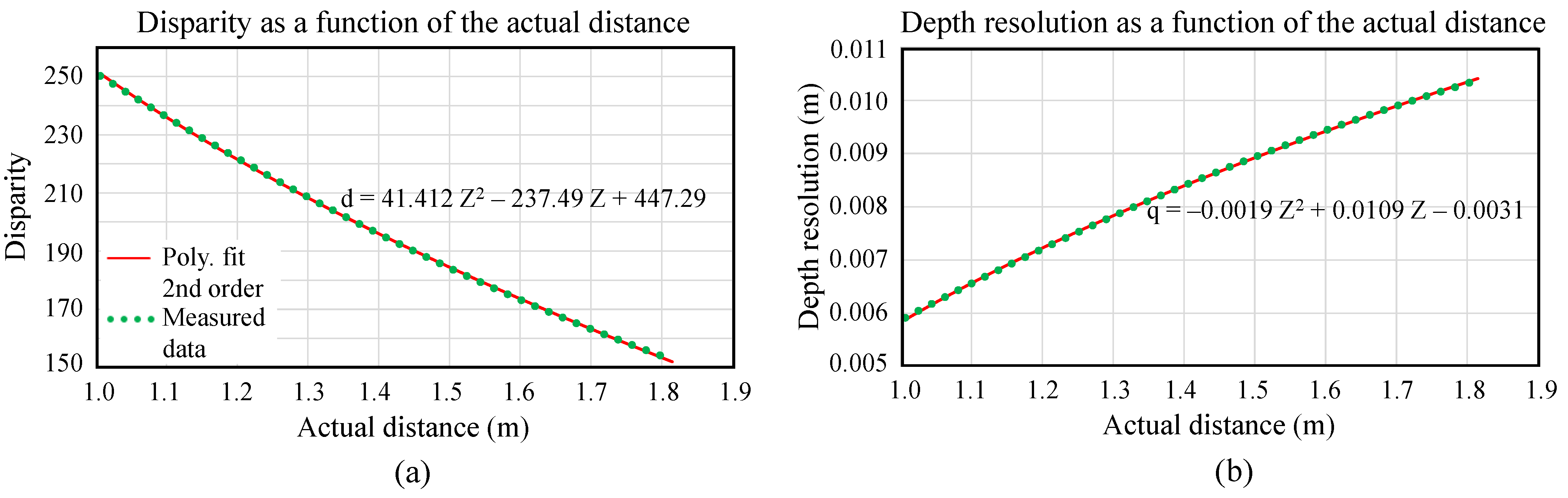
3.3. Point Cloud Creation from Disparity Values

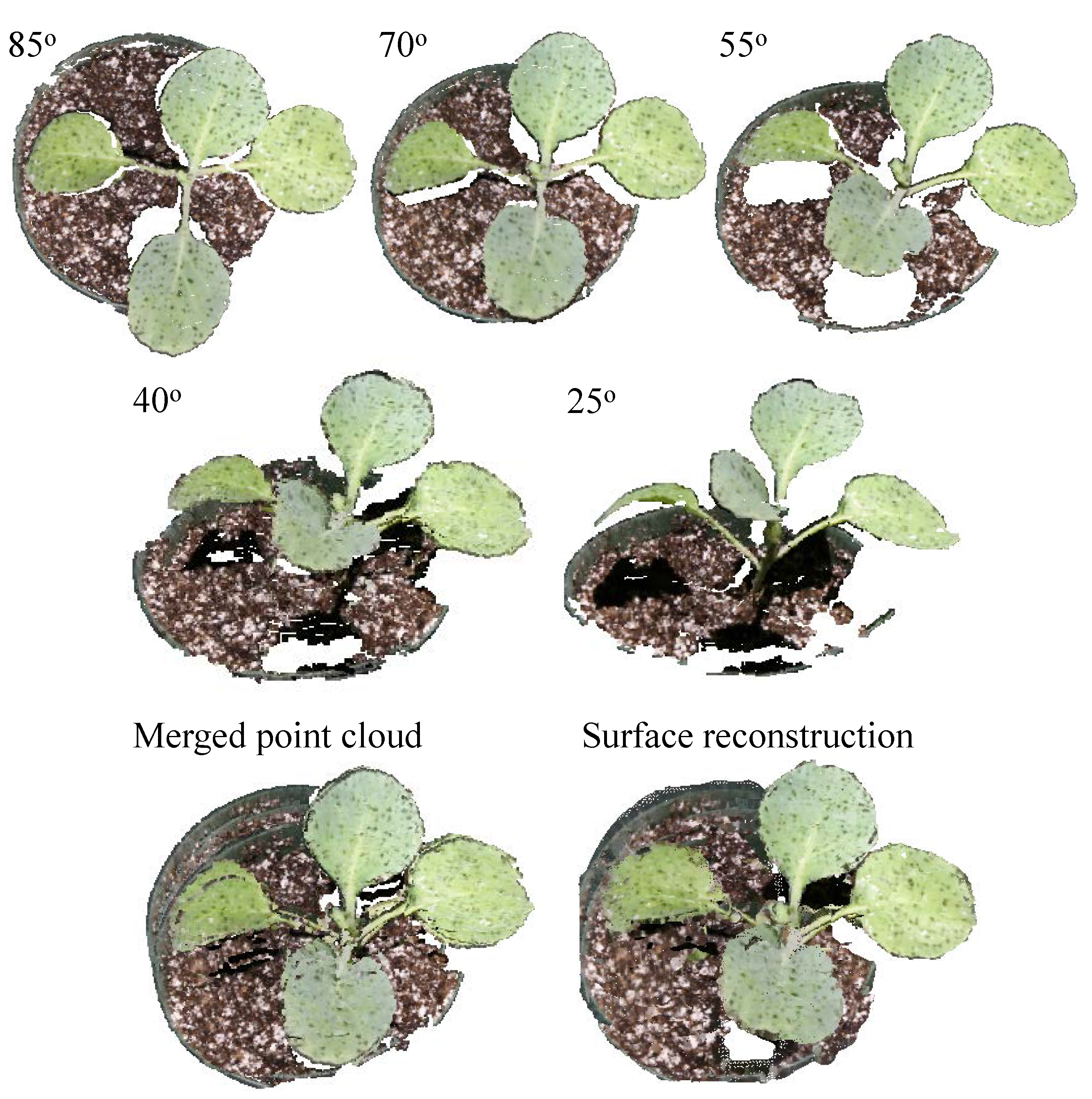
3.4. Point Cloud Registration

3.5. 3D Feature Extraction of a Plant
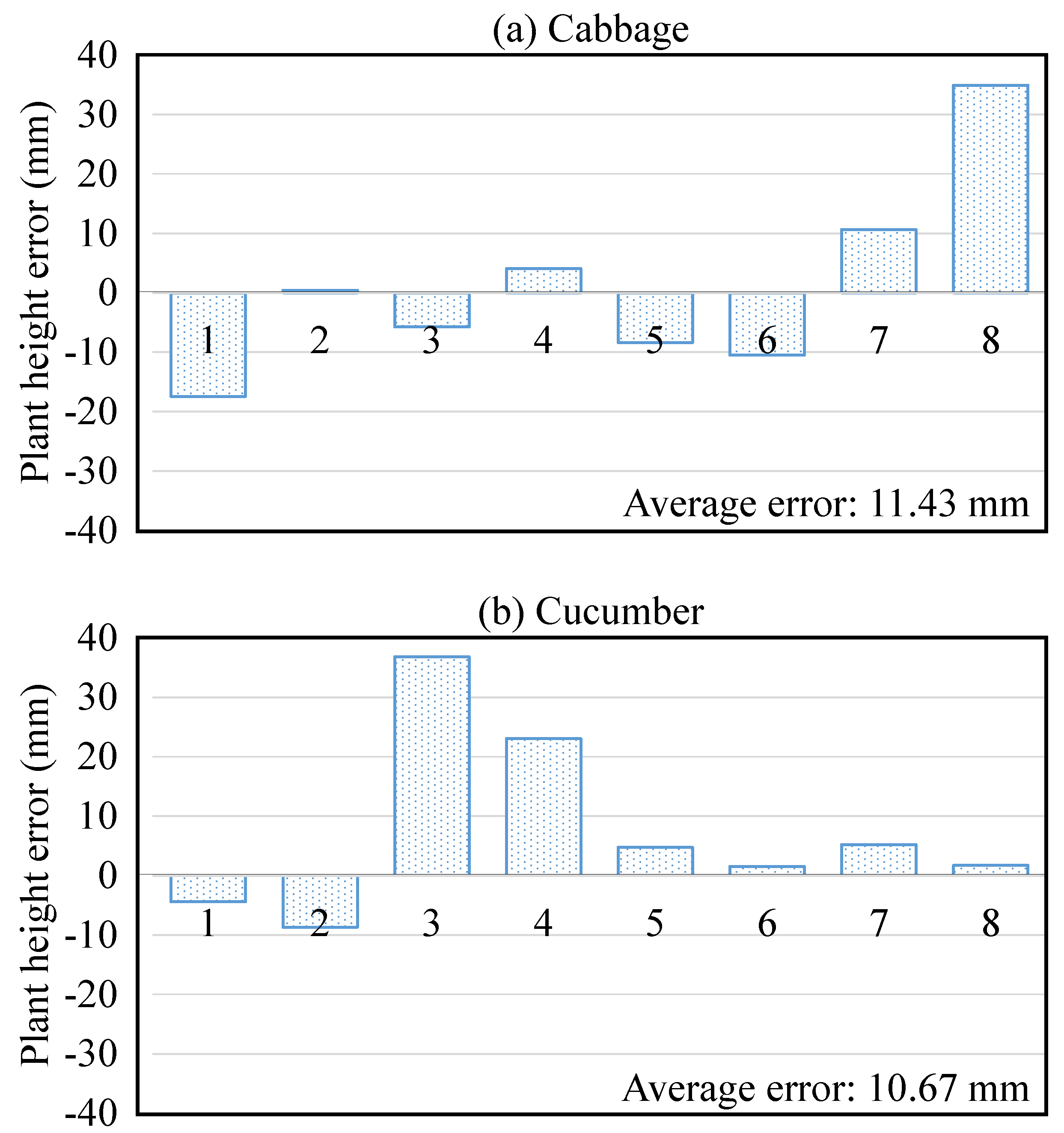
- Plant height: Plant height was defined as the absolute difference in the Z direction between the minimum and maximum 3D coordinates within the whole point cloud.
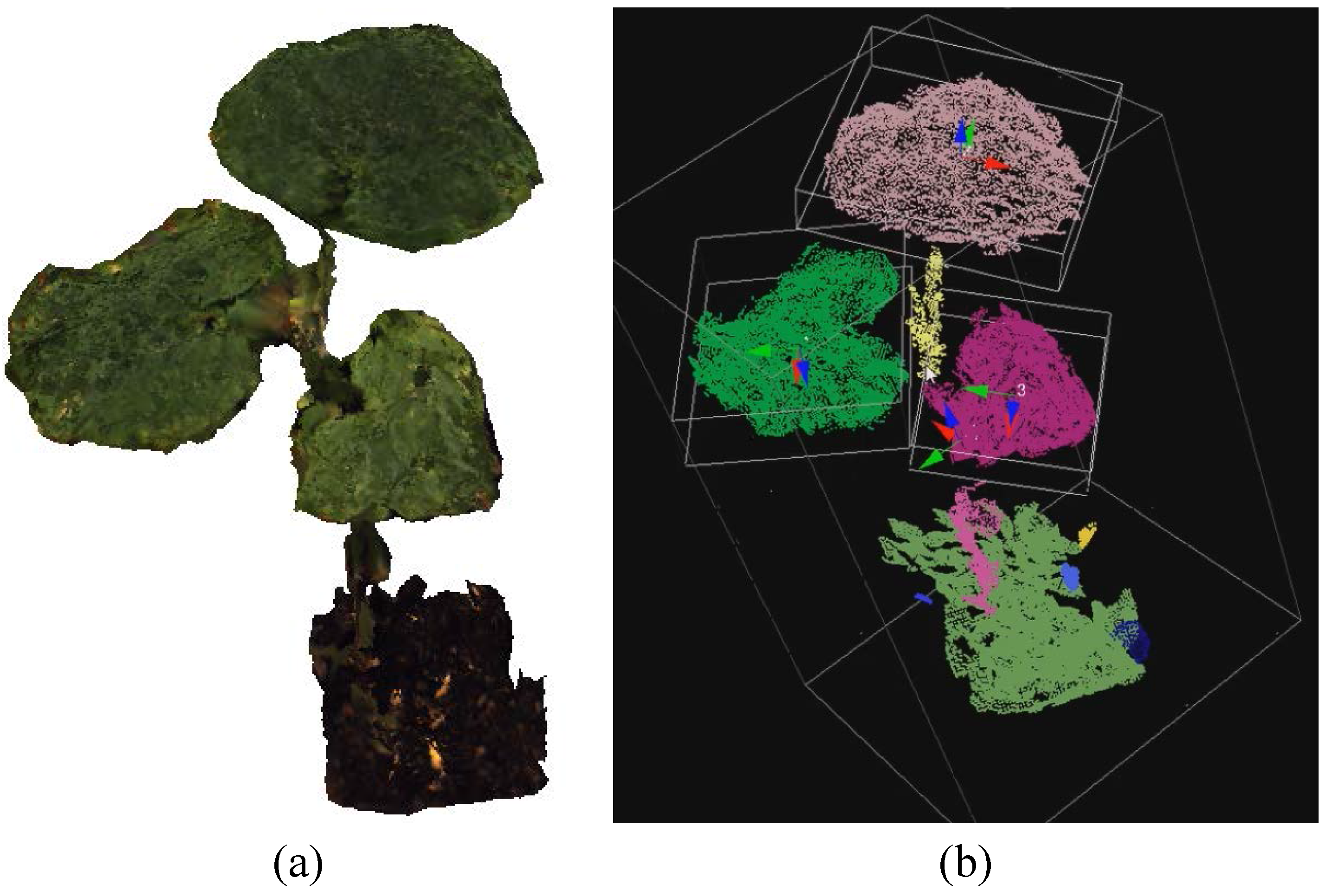
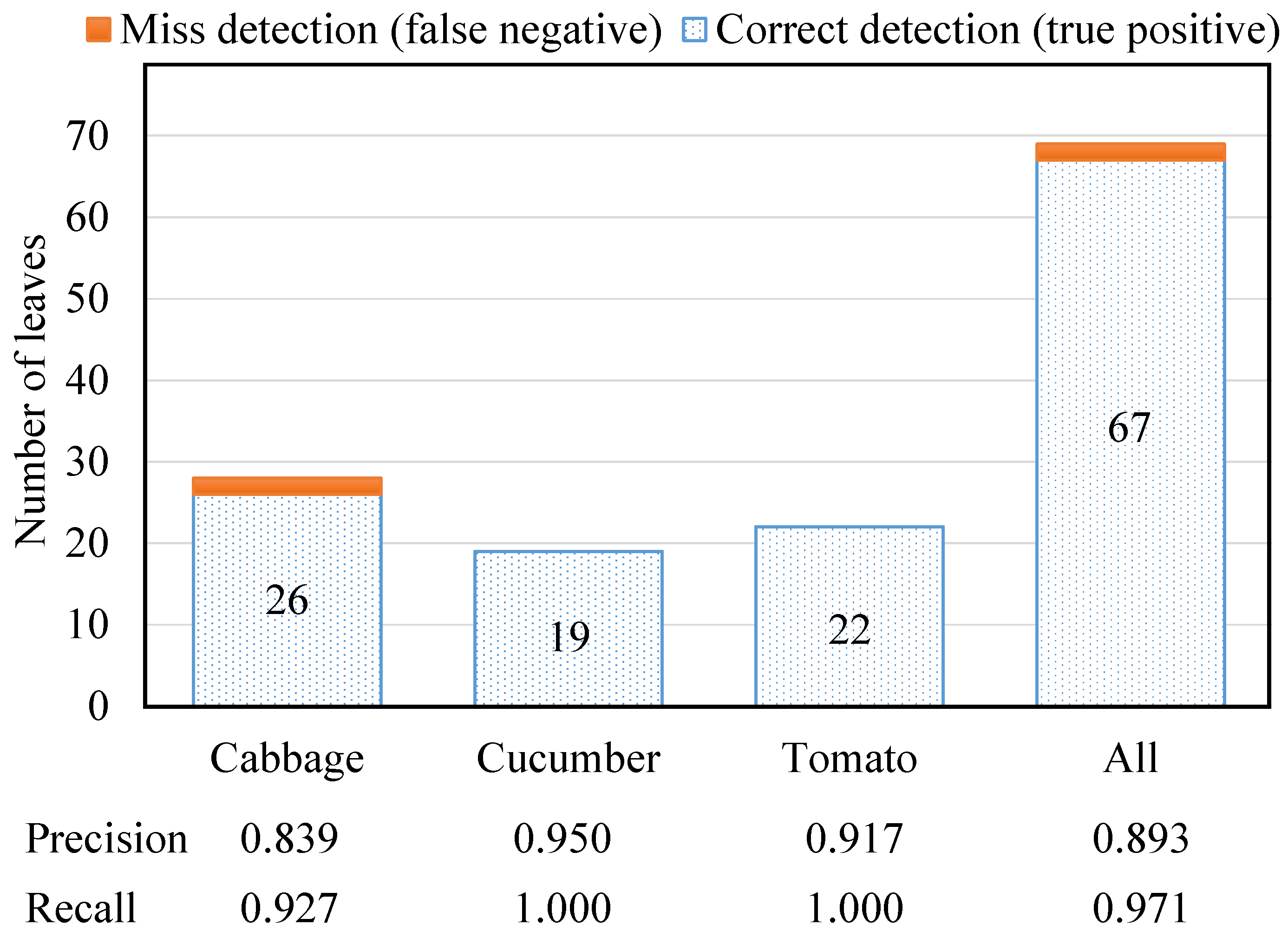
- Number of leaves/leaflets (leaf detection): To enumerate the number of leaves/leaflets, a cluster is considered a leaf/leaflet when these three Boolean conditions are satisfied:where is the maximum eigenvalue of the cluster; is the sum of all eigenvalues; and are thresholds for the conditions and , respectively; is a number defining locations for leaves; and implies that the magnitude of the dominant direction should not be much larger than that of other directions. Figure 8 shows a leaf detection result of a three-leaf cucumber plant, where its cloud is color-coded and displayed with bounding boxes using the Point Cloud Library [16].
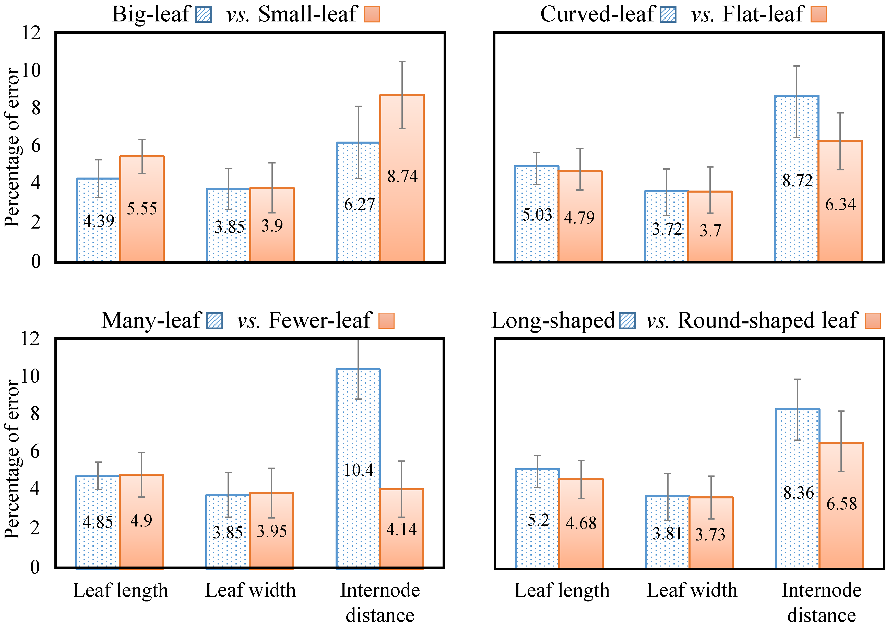
- Leaf size: Based on the detected leaves, a bounding box for each leaf is determined by using the leaf eigenvectors and centroid. The product of the width and length of the bounding box is defined as the leaf size.
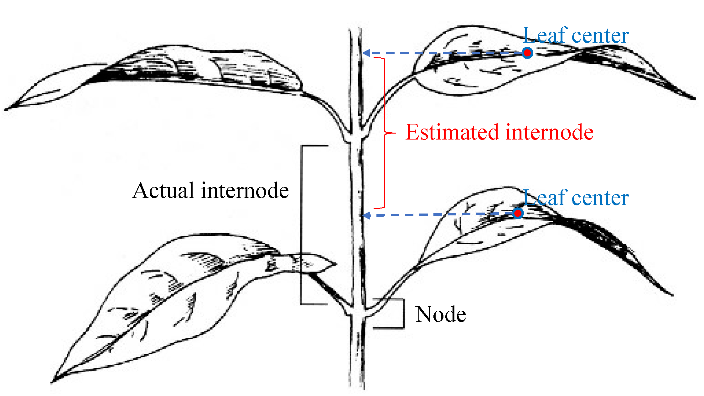
- Internode distance: The internode distance is the distance between two leaf nodes along a plant stem. Detecting nodes in a 3D point cloud is not a simple task; therefore, the following method is used to estimate the internode distances: leaf centers are projected onto the principal axis of the whole plant, then the distance between these projected points is considered as the internode distance. Figure 9 illustrates this method of internode distance estimation.
4. Experimental Results

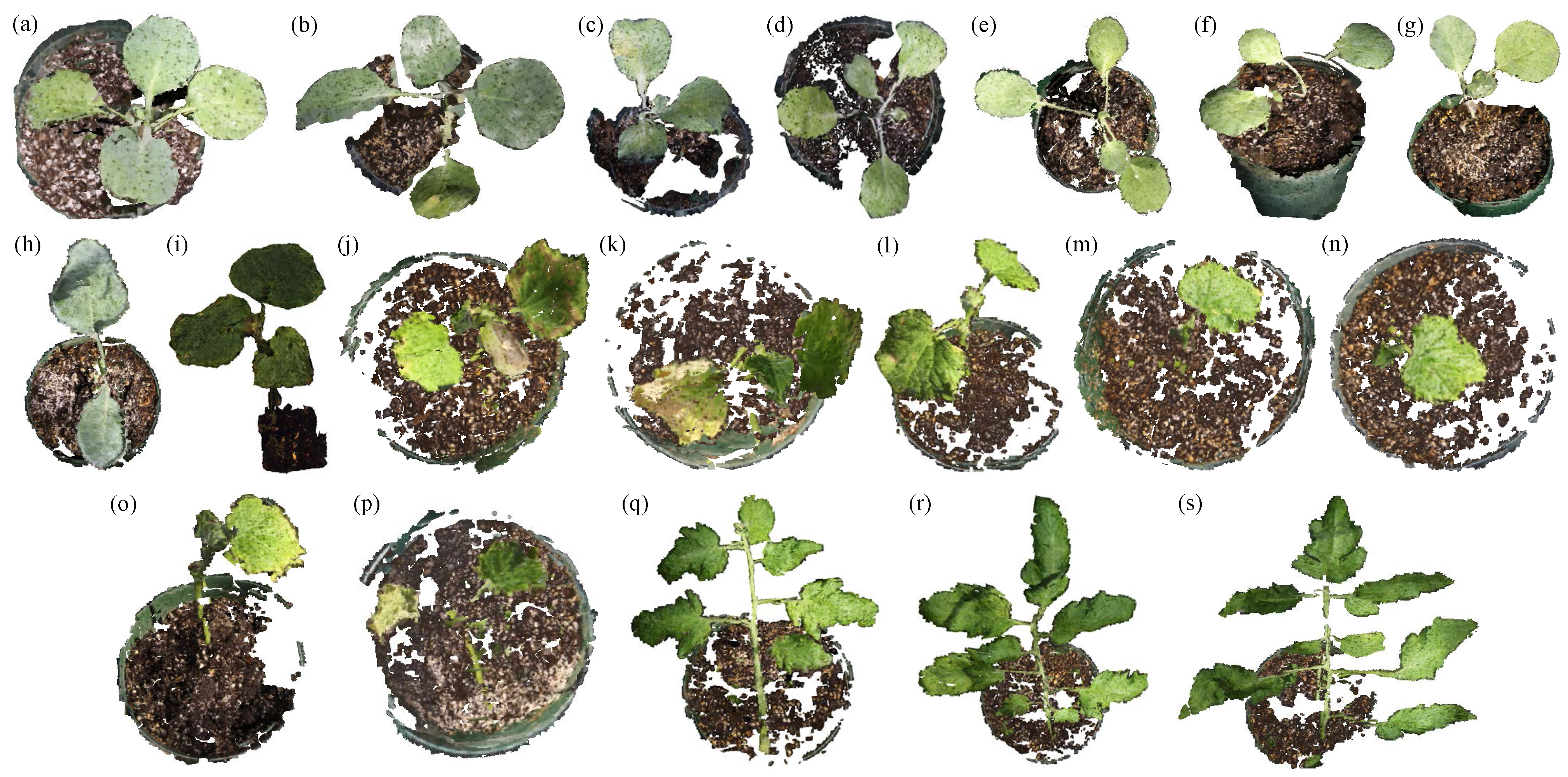
| Plant | Figure 10 | Height | No. of Leaves | Brief Description |
|---|---|---|---|---|
| Cabbage 1 | (a) | 114 | 4 | Good leaf shape |
| Cabbage 2 | (b) | 150 | 4 | 1 vertically-long leaf |
| Cabbage 3 | (c) | 140 | 4 | 1 small and 2 curved leaves |
| Cabbage 4 | (d) | 114 | 4 | Long branches |
| Cabbage 5 | (e) | 130 | 4 | 2 overlapped leaves |
| Cabbage 6 | (f) | 139 | 3 | Long and thin branches |
| Cabbage 7 | (g) | 105 | 3 | 1 leaf attaches to plant stem |
| Cabbage 8 | (h) | 229 | 2 | 1 curved leaf |
| Cucumber 1 | (i) | 242 | 3 | Tall, big leaves |
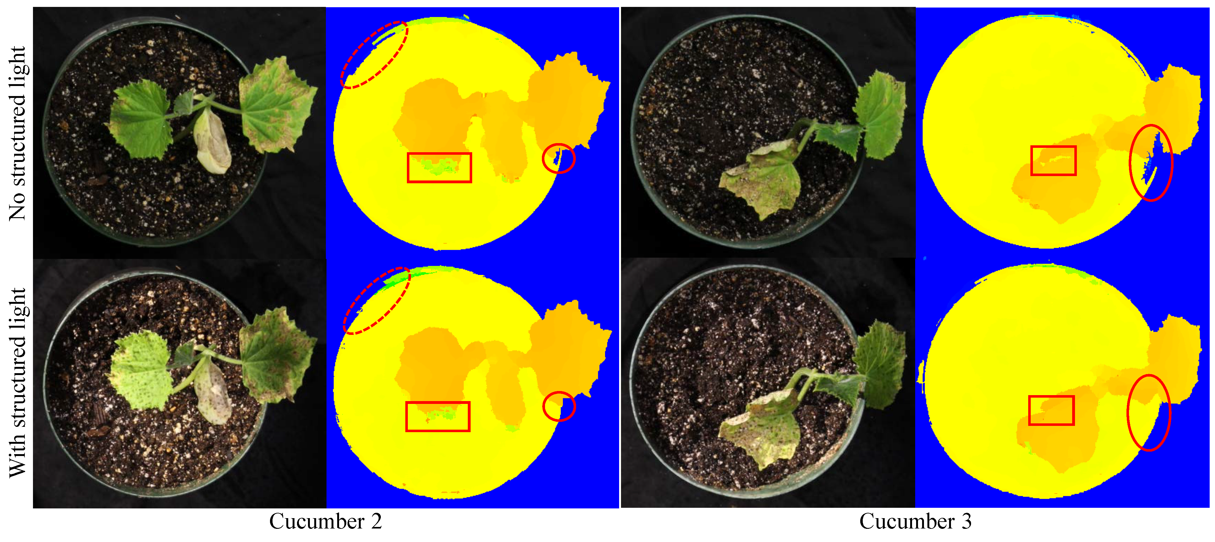
| Cucumber 2 | (j) | 117 | 4 | 2 brown-textured-surface leaves |
| Cucumber 3 | (k) | 131 | 3 | 2 brown-textured-surface leaves |
| Cucumber 4 | (l) | 115 | 2 | 1 small leaf |
| Cucumber 5 | (m) | 113 | 1 | Good leaf shape |
| Cucumber 6 | (n) | 123 | 2 | 1 small leaf |
| Cucumber 7 | (o) | 132 | 2 | 1 leaf attaches to plant stem |
| Cucumber 8 | (p) | 116 | 2 | 1 yellow-textured-surface leaf |
| Tomato 1 | (q) | 192 * | 6 | Long and curved leaves |
| Tomato 2 | (r) | 253 * | 8 | Long and curved leaves |
| Tomato 3 | (s) | 269 * | 8 | Long and curved leaves |
| GPU-Based Stereo Matching | Point Cloud Registration | 3D Feature Extraction * | ||||||||
|---|---|---|---|---|---|---|---|---|---|---|
| Plant segmentation | Spatial win-size | 11 | Registration | Max distance | 25 | Clustering | Tolerance | 0.03 | ||
| Color win-size | 7 | Max iteration | 10 | Min cluster size | 4000 | |||||
| Min segment size | 10 | Outlier rejection | 25 | Max cluster size | 10 | |||||
| Threshold | 10 | Poisson surface reconstruction | Octree depth | 12 | Leaf detection | Size threshold | 0.005 | |||
| Stereo block matching | No. of disparities | 256 | Solver divide | 7 | Direction threshold | 0.7 | ||||
| Win-size | 17 | Samples/node | 1 | Ratio: leaf location | 0.25 | |||||
| Texture threshold | 60 | Surface offset | 1 | * Parameters vary depending on leaf shape | ||||||
| Bilateral filter | Filter size | 41 | Face removal w.r.t. edge length | 0.05 | ||||||
| No. of iterations | 10 | Noise removal w.r.t. No. of faces | 25 | |||||||
| Plant Features | Cabbage | Cucumber | Tomato | Average | |
|---|---|---|---|---|---|
| Leaf height | Error (mm) | 6.86 | 5.08 | 10.16 | 6.6 |
| % error * | 5.58% | 4.36% | 4.36% | 4.87% | |
| Leaf width | Error (mm) | 5.08 | 4.83 | 5.33 | 5.08 |
| % error * | 4.16% | 3.9% | 2.31% | 3.76% | |
| Internode distance | Error (mm) | 9.65 | 7.87 | 21.34 | 10.92 |
| % error * | 7.67% | 6.3% | 8.49% | 7.28% | |

| Study | Camera System | Camera View | Measures | Environment | Techniques | Accuracy | Processing Time |
|---|---|---|---|---|---|---|---|
| Alenya, 2011 [13] | ToF and color cameras; robot arm | Multiview for leaf modeling | Leaf size | Indoor | Depth-aided color segmentation, quadratic surface fitting, leaf localization | Square fitting error: 2 cm2 | 1 min for 3D leaf segmentation |
| Chene, 2012 [18] | Kinect camera | Top view | Leaf azimuth | Indoor | Maximally stable extremal regions-based leaf segmentation | Detection accuracy 68%; azimuth error 5% | n/a |
| Heijden, 2012 [39] | ToF and color cameras | Single view | Leaf size and angle | Greenhouse (for large pepper plants) | Edge-based leaf detection, locally weighted scatterplot smoothing-based surface reconstruction | Leaf height correlation 0.93; leaf area correlation 0.83 | 3 min for image recording, hours for the whole process |
| Paproki, 2012 [19] | High-resolution SLR camera, with 3D modeling software [20] | Multiview for full 3D reconstruction | Plant height, leaf width and length | Indoor | Constrained region growing, tubular shape fitting-based stem segmentation, planar-symmetry and normal clustering-based leaf segmentation, pair-wise matching-based temporal analysis | Plant height error 9.34%; leaf width error 5.75%; leaf length error 8.78% | 15 min for 3D reconstruction [20], 4.9 min for 3D mesh processing and plant feature analysis |
| Azzari, 2013 [15] | Kinect camera | Top view | Plant height, base diameter | Outdoor | Canopy structure extraction | Correlation: 0.97 | n/a |
| Ni, 2014 [12] | 2 low-resolution stereo cameras with 3D modeling software [7] | Multiview for full 3D reconstruction | Plant height and volume, leaf area | Indoor | Utilizing VisualSFM software [7], utilizing [40] to manually extract plant features | n/a | n/a |
| Song, 2014 [14] | Two stereo cameras; ToF camera | Single view | Leaf area (foreground leaves only) | Greenhouse (for large plants) | Dense stereo with localized search, edge-based leaf detection, locally weighted scatterplot smoothing-based surface reconstruction | Error: 9.3% | 5 min for the whole process |
| Polder, 2014 [23] | 3D light-field camera | Single view | Leaf and fruit detection | Greenhouse (for large tomato plants) | Utilizing 3D light-field camera to output a pixel to pixel registered color image and depth map | n/a | n/a |
| Rose, 2015 [22] | High-resolution SLR camera, with 3D modeling software [41] | Multiview for full 3D reconstruction | Plant height, leaf area, convex hull | Indoor | Utilizing Pix4Dmapper software [41] to have 3D models, plant feature extraction | Correlation: 0.96 | 3 min for data acquisition, 20 min for point cloud generation, 5 min for manual scaling, 10 min for error removal |
| Andujar, 2015 [21] | 4 Kinect cameras with 3D modeling software [42] | Multiview for semi-full 3D reconstruction | Plant height, leaf area, biomass | Outdoor | Utilizing Skanect software [42] to have 3D models, utilizing [40] to manually extract plant features | Correlation: plant height 0.99, leaf area 0.92, biomass 0.88 | n/a |
| Our system | 10 high-resolution SLR cameras organized into 5 stereo pairs; 2 structured lights | Multiview for full 3D reconstruction | Plant height, leaf width and length, internode distance | Indoor | Texture creation using structured lights, mean shift-based plant segmentation, stereo block matching, disparity bilateral filtering, ICP-based point cloud registration, Poisson surface reconstruction, plant feature extraction | Leaf detection accuracy 97%; plant height error 8.1%, leaf width error 3.76%, leaf length error 4.87%, internode distance error 7.28% | 4 min for the whole process |
5. Conclusions and Future Work
Acknowledgments
Author Contributions
Conflicts of Interest
References
- Dhondt, S.; Wuyts, N.; Inze, D. Cell to whole-plant phenotyping: The best is yet to come. Trends Plant Sci. 2013, 18, 428–439. [Google Scholar] [CrossRef] [PubMed]
- Furbank, R.T.; Tester, M. Phenomics-technologies to relieve the phenotyping bottleneck. Trends Plant Sci. 2011, 16, 635–644. [Google Scholar] [CrossRef] [PubMed]
- Scotford, I.M.; Miller, P.C.H. Applications of spectral reflectance techniques in northern European cereal production: A review. Biosyst. Eng. 2005, 90, 235–250. [Google Scholar] [CrossRef]
- Garrido, M.; Perez-Ruiz, M.; Valero, C.; Gliever, C.J.; Hanson, B.D.; Slaughter, D.C. Active optical sensors for tree stem detection and classification in nurseries. Sensors 2014, 14, 10783–10803. [Google Scholar] [CrossRef] [PubMed]
- Slaughter, D.C.; Giles, D.K.; Downey, D. Autonomous robotic weed control systems: A review. Comput. Electron. Agric. 2008, 61, 63–78. [Google Scholar] [CrossRef]
- Cui, Y.; Schuon, S.; Chan, D.; Thrun, S.; Theobalt, C. 3D shape scanning with a time-of-flight camera. In Proceedings of the 2010 IEEE Conference on Computer Vision and Pattern Recognition (CVPR), San Francisco, CA, USA, 13–18 June 2010; pp. 1173–1180.
- Wu, C. Towards linear-time incremental structure from motion. In Proceedings of the 2013 International Conference on 3D Vision, Seattle, WA, USA, 29 June–1 July 2013; pp. 127–134.
- Li, J.; Miao, Z.; Liu, X.; Wan, Y. 3D reconstruction based on stereovision and texture mapping. In Proceedings of the ISPRS Technical Commission III Symposium, Photogrammetric Computer Vision and Image Analysis, Paris, France, 1–3 September 2010; pp. 1–6.
- Brandou, V.; Allais, A.; Perrier, M.; Malis, E.; Rives, P.; Sarrazin, J.; Sarradin, P.M. 3D reconstruction of natural underwater scences using the stereovision system IRIS. In Proceedings of the Europe OCEANS, Aberdeen, Hong Kong, China, 18–21 June 2007; pp. 1–6.
- Zhang, Z. Microsoft Kinect sensor and its effect. IEEE Multimed. 2012, 19, 4–12. [Google Scholar] [CrossRef]
- Newcombe, R.A.; Davison, A.J.; Izadi, S.; Kohli, P.; Hilliges, O.; Shotton, J.; Molyneaux, D.; Hodges, S.; Kim, D.; Fitzgibbon, A.; et al. KinectFusion: Real-time dense surface mapping and tracking. In Proceedings of the 2011 10th IEEE International Symposium on Mixed and Augmented Reality, Basel, Switzerland, 26–29 October 2011; pp. 127–136.
- Ni, Z.; Burks, T.F.; Lee, W.S. 3D reconstruction of small plant from multiple views. In Proceedings of the ASABE and CSBE/SCGAB Annual International Meeting, Montreal, QC, Canada, 13–16 July 2014.
- Alenya, G.; Dellen, B.; Torras, C. 3D modelling of leaves from color and ToF data for robotized plant measuring. In Proceedings of the 2011 IEEE International Conference on Robotics and Automation (ICRA), Shanghai, China, 9–13 May 2011; pp. 3408–3414.
- Song, Y.; Glasbey, C.A.; Polder, G.; van der Heijden, G.W.A.M. Non-destructive automatic leaf area measurements by combining stereo and time-of-flight images. IEEE Multimed. 2014, 8, 391–403. [Google Scholar] [CrossRef]
- Azzari, G.; Goulden, M.L.; Rusu, R.B. Rapid characterization of vegetation structure with a Microsoft Kinect sensor. Sensors 2013, 13, 2384–2398. [Google Scholar] [CrossRef] [PubMed]
- Rusu, R.B.; Cousins, S. 3D is here: Point cloud library (PCL). In Proceedings of the 2011 IEEE International Conference on Robotics and Automation (ICRA), Shanghai, China, 9–13 May 2011; pp. 1–4.
- Li, D.; Xu, L.; Tan, C.; Goodman, E.D.; Fu, D.; Xin, L. Digitization and visualization of greenhouse tomato plants in indoor environments. Sensors 2015, 15, 4019–4051. [Google Scholar] [CrossRef] [PubMed]
- Chene, Y.; Rousseau, D.; Lucidarme, P.; Bertheloot, J.; Caffier, V.; Morel, P.; Belin, E.; Chapeau-Blondeau, F. On the use of depth camera for 3D phenotyping of entire plants. Comput. Electron. Agric. 2012, 82, 122–127. [Google Scholar] [CrossRef]
- Paproki, A.; Sirault, X.; Berry, S.; Furbank, R.; Fripp, J. A novel mesh processing based technique for 3D plant analysis. BMC Plant Biol. 2012, 12, 1–13. [Google Scholar] [CrossRef] [PubMed]
- Baumberg, A.; Lyons, A.; Taylor, R. 3D S.O.M.—A commercial software solution to 3D scanning. Graph. Models 2005, 67, 476–495. [Google Scholar] [CrossRef]
- Andujar, D.; Fernandez-Quintanilla, C.; Dorado, J. Matching the best viewing angle in depth cameras for biomass estimation based on poplar seedling geometry. Sensors 2015, 15, 12999–13011. [Google Scholar] [CrossRef] [PubMed]
- Rose, J.C.; Paulus, S.; Kuhlmann, H. Accuracy analysis of a multi-view stereo approach for phenotyping of tomato plants at the organ level. Sensors 2015, 15, 9651–9665. [Google Scholar] [CrossRef] [PubMed]
- Polder, G.; Hofstee, J.W. Phenotyping large tomato plants in the greenhouse using a 3D light-field camera. In Proceedings of the ASABE and CSBE/SCGAB Annual International Meeting, Montreal, QC, Canada, 13–16 July 2014.
- Paulus, S.; Dupuis, J.; Mahlein, A.K.; Kuhlmann, H. Surface feature based classification of plant organs from 3D laser scanned point clouds for plant phenotyping. BMC Bioinform. 2013, 14, 1–12. [Google Scholar] [CrossRef] [PubMed]
- Paulus, S.; Dupuis, J.; Riedel, S.; Kuhlmann, H. Automated analysis of barley organs using 3D laser scanning: An approach for high throughput phenotyping. Sensors 2014, 14, 12670–12686. [Google Scholar] [CrossRef] [PubMed]
- digiCamControl—Free Windows DSLR Camera Controlling Solution. Available online: http://digicamcontrol.com (accessed on 24 July 2015).
- Zhang, Z. A flexible new technique for camera calibration. IEEE Trans. Pattern Anal. Mach. Intell. 2000, 22, 1330–1334. [Google Scholar] [CrossRef]
- Bouguet, J.Y. Camera Calibration Toolbox for Matlab; California Institute of Technology: Pasadena, CA, USA, 2013. [Google Scholar]
- Comaniciu, D.; Meer, P. Mean shift: A robust approach toward feature space analysis. IEEE Trans. Pattern Anal. Mach. Intell. 2002, 24, 603–619. [Google Scholar] [CrossRef]
- Men, L.; Huang, M.; Gauch, J. Accelerating mean shift segmentation algorithm on hybrid CPU/GPU platforms. In Proceedings of the International Workshop Modern Accelerator Technologies for GIScience, Columbus, OH, USA, 18–21 September 2012.
- Felzenszwalb, P.F.; Huttenlocher, D.P. Efficient belief propagation for early vision. Int. J. Comput. Vis. 2006, 70, 972–986. [Google Scholar] [CrossRef]
- Nguyen, V.D.; Nguyen, T.T.; Nguyen, D.D.; Lee, S.J.; Jeon, J.W. A fast evolutionary algorithm for real-time vehicle detection. IEEE. Trans. Veh. Technol. 2013, 62, 2453–2468. [Google Scholar] [CrossRef]
- Taniai, T.; Matsushita, Y.; Naemura, T. Graph cut based continuous stereo matching using locally shared labels. In Proceedings of the 2014 IEEE Conference on Computer Vision and Pattern Recognition (CVPR), Columbus, OH, USA, 23–28 June 2014.
- Nguyen, V.D.; Nguyen, T.T.; Nguyen, D.D.; Jeon, J.W. Adaptive ternary-derivative pattern for disparity enhancement. In Proceedings of the 19th IEEE International Conference on Image Processing (ICIP), Orlando, FL, USA, 30 September–3 October 2012; pp. 2969–2972.
- Nguyen, V.D.; Nguyen, D.D.; Nguyen, T.T.; Dinh, V.Q.; Jeon, J.W. Support local pattern and its application to disparity improvement and texture classification. IEEE Trans. Circuit Syst. Video Technol. 2014, 24, 263–276. [Google Scholar] [CrossRef]
- Yang, Q.; Wang, L.; Ahuja, N. A constant-space belief propagation algorithm for stereo matching. In Proceedings of the 2010 IEEE Conference on Computer Vision and Pattern Recognition (CVPR), San Francisco, CA, USA, 13–18 June 2010; pp. 1458–1465.
- Aiger, D.; Mitra, N.J.; Cohen-Or, D. 4-Points congruent for robust surface registration. ACM Trans. Graph. 2008, 27, 1–10. [Google Scholar] [CrossRef]
- Rusu, R.B. Semantic 3D Object Maps for Everyday Manipulation in Human Living Environments. PhD Thesis, Computer Science Department, Technische Universitaet Muenchen, Munich, Germany, 2009. [Google Scholar]
- Heijden, G.; Song, Y.; Horgan, G.; Polder, G.; Dieleman, A.; Bink, M.; Palloix, A.; Eeuwijk, F.; Glasbey, C. SPICY: Towards automated phenotyping of large pepper plants in the greenhouse. Funct. Plant Biol. 2012, 39, 870–877. [Google Scholar] [CrossRef]
- MeshLab. Available online: http://meshlab.sourceforge.net (accessed on 24 July 2015).
- Pix4D UAV Mapping Photogrammetry Software, Pix4Dmapper. Available online: https://pix4d.com (accessed on 24 July 2015).
- Skanect 3D Scanning Software by Occipital. Available online: http://skanect.occipital.com (accessed on 24 July 2015).
© 2015 by the authors; licensee MDPI, Basel, Switzerland. This article is an open access article distributed under the terms and conditions of the Creative Commons Attribution license (http://creativecommons.org/licenses/by/4.0/).
Share and Cite
Nguyen, T.T.; Slaughter, D.C.; Max, N.; Maloof, J.N.; Sinha, N. Structured Light-Based 3D Reconstruction System for Plants. Sensors 2015, 15, 18587-18612. https://doi.org/10.3390/s150818587
Nguyen TT, Slaughter DC, Max N, Maloof JN, Sinha N. Structured Light-Based 3D Reconstruction System for Plants. Sensors. 2015; 15(8):18587-18612. https://doi.org/10.3390/s150818587
Chicago/Turabian StyleNguyen, Thuy Tuong, David C. Slaughter, Nelson Max, Julin N. Maloof, and Neelima Sinha. 2015. "Structured Light-Based 3D Reconstruction System for Plants" Sensors 15, no. 8: 18587-18612. https://doi.org/10.3390/s150818587
APA StyleNguyen, T. T., Slaughter, D. C., Max, N., Maloof, J. N., & Sinha, N. (2015). Structured Light-Based 3D Reconstruction System for Plants. Sensors, 15(8), 18587-18612. https://doi.org/10.3390/s150818587