1. Introduction
GNSS precise point positioning (PPP) has proven to be capable of providing positioning accuracy at the sub-decimeter and decimeter levels in static and kinematic modes, respectively. PPP accuracy and convergence time are controlled by the ability to mitigate all potential error biases in the system. Several comprehensive studies have been published on the accuracy and convergence time of un-differenced GPS and GPS/Galileo PPP models (see for example, [
1,
2,
3,
4,
5,
6]. In the traditional un-differenced GPS PPP model, because of the presence of the un-calibrated hardware delays, the ambiguity parameters are typically obtained as real-value numbers [
4,
5,
7,
8]. This in turn affects the GPS PPP solution convergence and accuracy [
9]. However, recent research has demonstrated that the correct integer values for the ambiguity parameters can be recovered if the satellite hardware delays can be calibrated.
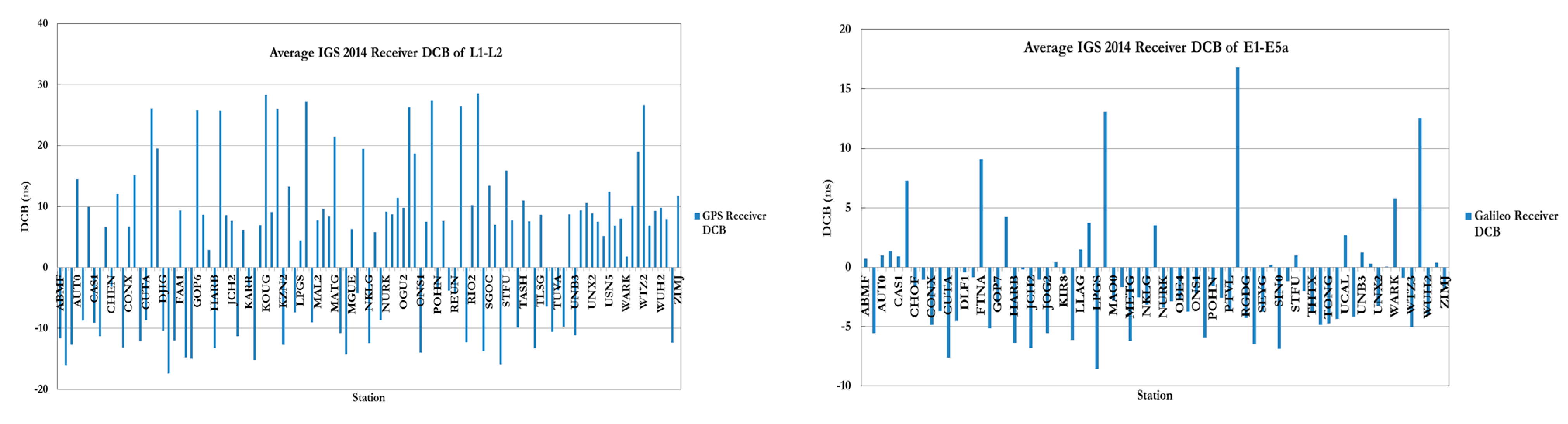
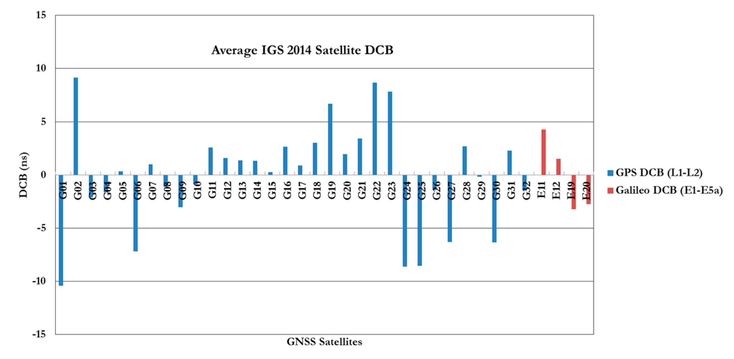
Figure 1 and
Figure 2 show the IGS average estimated values of the receiver and satellite differential code biases, respectively, for 2014 [
10]. As can be seen in
Figure 2, Galileo satellite differential code biases of E1/E5a signals are relatively smaller than the GPS L1/L2 counterpart.
Figure 1.
Average 2014 IGS receiver DCB for GPS and Galileo signals.
Figure 1.
Average 2014 IGS receiver DCB for GPS and Galileo signals.
Figure 2.
Average IGS 2014 satellite DCB for both GPS/Galileo signals.
Figure 2.
Average IGS 2014 satellite DCB for both GPS/Galileo signals.
For a single GNSS constellation, between-satellite single-difference (BSSD) linear combination cancels out all receiver-related errors, including the receiver hardware delays, which significantly improves the convergence time [
3,
4,
11,
12]. This, however, is not the case when the measurements of two or more constellations are combined. When forming BSSD for GPS and Galileo measurements, three scenarios can be considered on the selection of the reference satellite. Either a GPS or a Galileo satellite is selected as a reference for both GPS and Galileo observables. Alternatively, two reference satellites are selected: a GPS reference satellite for the GPS observables and a Galileo satellite for the Galileo observables. The first approach is commonly referred to as tight combination, while the latter is commonly referred to as per-constellation or loose combination [
6].
This paper examines the performance of several PPP models, which combine the dual-frequency GPS/Galileo observables in both un-differenced and BSSD mode. The IGS-MGEX network products used to correct for the satellite differential code biases, the orbital and satellite clock errors [
13]. As the IGS-MGEX products are presently referenced to the GPS time and since we use mixed GNSS receivers that also use the GPS time as a reference, the GPS to Galileo time offset (GGTO) is cancelled out in our models. The inter-system bias is either cancelled out through differencing the observations or is treated as an additional unknown parameter. The Hopfield tropospheric correction model is used, along with the Vienna mapping function, to account for the hydrostatic component of the tropospheric delay [
14,
15]. The wet component is treated as an additional unknown parameter in the estimation model. Other corrections are also applied, including the effect of ocean loading [
16,
17], Earth tide [
18], carrier-phase windup [
19,
20], Sagnac [
21], relativity [
22], and satellite and receiver antenna phase-center variations [
23]. Natural Resources Canada’s GPSPace PPP software is modified to handle the various GPS/Galileo PPP models. A total of six data sets of GPS and Galileo observations at six IGS stations are processed to examine the performance of the various PPP models. It is shown that the traditional un-differenced GPS/Galileo PPP model, the GPS decoupled clock model, and semi-decoupled clock GPS/Galileo PPP model improve the convergence time by about 25% in comparison with the un-differenced GPS-only model. In addition, the semi-decoupled GPS/Galileo PPP model improves the solution precision by about 25% compared to the traditional un-differenced GPS/Galileo PPP model. Moreover, the BSSD GPS/Galileo PPP model improves the solution convergence time by about 50%, in comparison with the un-differenced GPS PPP model, regardless of the type of BSSD combination used. As well, the BSSD model improves the precision of the estimated parameters by about 50% and 25% when the loose and the tight combinations are used, respectively, in comparison with the un-differenced GPS-only model. Comparable results are obtained through the tight combination when either a GPS or a Galileo satellite is selected as a reference.
4. Least Squares Estimation Technique
Under the assumption that the observations are uncorrelated and the errors are normally distributed with zero mean, the covariance matrix of the un-differenced observations takes the form of a diagonal matrix. The elements along the diagonal line represent the variances of the code and carrier phase measurements. Following the common practice, the ratio between the standard deviations of the code and the carrier-phase measurements is taken as 100. When forming BSSD, however, the differenced observations become mathematically correlated. This leads to a fully populated covariance matrix at a particular epoch.
The general linearized form for the above observation equations around the initial (approximate) vector
u0 and observables
𝑙 can be written in a compact form as:
where
u is the vector of unknown parameters;
A is the design matrix, which includes the partial derivatives of the observation equations with respect to the unknown parameters
u;
Δu is the unknown vector of corrections to the approximate parameters
u0,
i.e.,
u =
u0 +
Δu;
w is the misclosure vector and
r is the vector of residuals. The sequential least-squares solution for the unknown parameters
Δui at an epoch
i can be obtained from [
26]:
where
Δui−1 is the least-squares solution for the estimated parameters at epoch
i − 1;
M is the matrix of the normal equations;
Cl and
CΔu are the covariance matrices of the observations and unknown parameters, respectively. It should be pointed out that the usual batch least-squares adjustment should be used in the first epoch,
i.e., for
i = 1. The batch solution for the estimated parameters and the inverse of the normal equation matrix are given, respectively, by [
26]:
where
Cx0 is the
a priori covariance matrix for the approximate values of the unknown parameters.
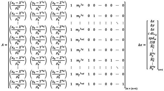
In case of the traditional GPS/Galileo PPP model, the design matrix
A and the vector of corrections to the unknown parameters Δ
x take the following forms:
where
nG refers to the number of visible GPS satellites;
nE refers to the number of visible Galileo satellites;
n =
nG +
nE is the total number of the observed satellites for both GPS/Galileo systems;
x0,
y0 and
z0 are the approximate receiver coordinates;
are the known GPS satellite coordinates;
are the known Galileo satellite coordinates;
ρ0 is the approximate receiver-satellite range. The unknown parameters in the above system are the corrections to the receiver coordinates, Δ
x, Δ
y, and Δ
z, the wet component of the tropospheric zenith path delay
zpdw, the inter-system bias
ISB, and the non-integer ambiguity parameters
.
For the decoupled clock model, the design matrix
A and the vector of corrections to the unknown parameters Δ
x take the following forms:
where
and
are the pseudorange and carrier phase receiver clock errors, respectively;
and
are the pseudorange and carrier phase inter-system bias, respectively.
For the un-differenced semi-decoupled clock GPS/Galileo PPP model, the design matrix
A and the vector of corrections to the unknown parameters Δ
x take the same form as the decoupled clock GPS/Galileo model given in Equation (102). When a GPS satellite is selected as a reference to form the BSSD for GPS/Galileo observations, the design matrix
A and the vector of corrections
Δu take the form:
where “
1G” refers to the GPS reference satellite.
By analogy, the use of a Galileo satellite as a reference to form the BSSD for both of the GPS and Galileo observations leads to:
where
1E refers to the Galileo reference satellite.
When two reference satellites are selected to form the BSSD,
i.e., per-constellation BSSD, the design matrix
A and the vector of corrections
Δu take the form:
The major advantage of the above per-constellation (or loose combination) system is that the modified receiver clock error and the inter-system bias are cancelled out. Similarly, the design matrix
A and the vector of corrections
Δu for the BSSD decoupled clock model, with a GPS satellite selected as a reference, take the form:
where “
1G” refers to the GPS reference satellite.
If, however, a Galileo satellite is selected as a reference, the design matrix
A and the vector of corrections
Δu for the BSSD decoupled clock model take the form:
where
1E refers to the Galileo reference satellite. For the per-constellation BSSD decoupled clock model, the design matrix
A and the vector of corrections
Δu will take the same form as those of the traditional BSSD GPS/Galileo PPP model. For the BSSD semi-decoupled clock GPS/Galileo PPP model, the design matrix
A and the vector of corrections to the unknown parameters Δ
x will be the same as those of the BSSD decoupled clock model.
5. Results and Discussion
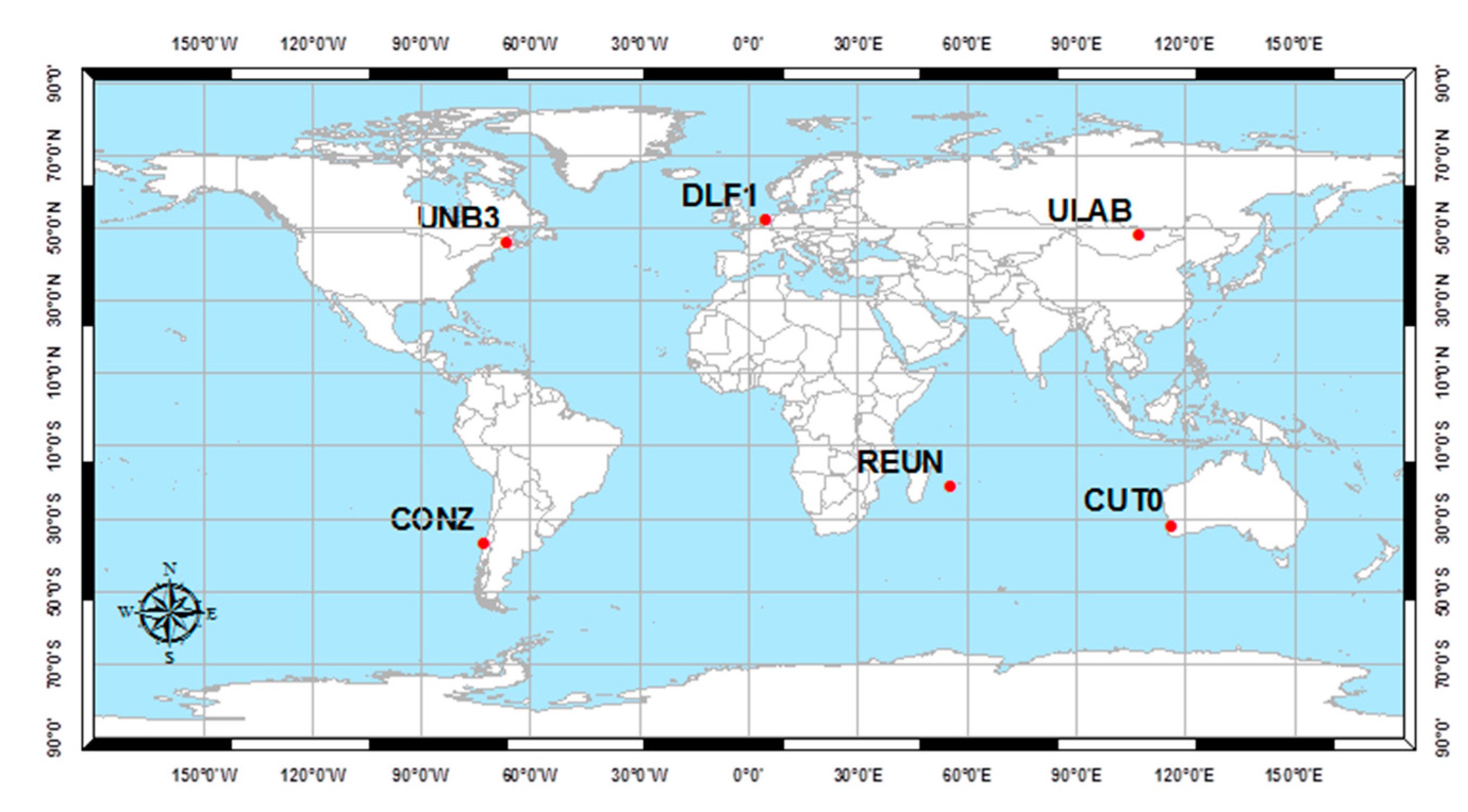
To verify the introduced GPS/Galileo PPP models, GPS/Galileo measurements at six well-distributed stations (
Figure 6) were selected from the IGS tracking network [
23]. Those stations are occupied by GNSS receivers, which are capable of simultaneously tracking the GPS/Galileo constellations. The positioning results for station DLF1 are presented below. Similar results are obtained from the other stations. However, a summary of the convergence times and precision are presented below for all stations. Natural Resources Canada (NRCan) GPSPace PPP software was modified to enable a GPS/Galileo PPP solution as described above. A solution is considered to be converged when the three-dimensional positioning standard deviation reaches 10 cm. The sampling interval for all data sets is 30 s of 5 April 2013, while the time span used in the analysis is one hour, which is selected to ensure that the four Galileo satellites are visible at each station.
Figure 6.
Analysis stations.
Figure 6.
Analysis stations.
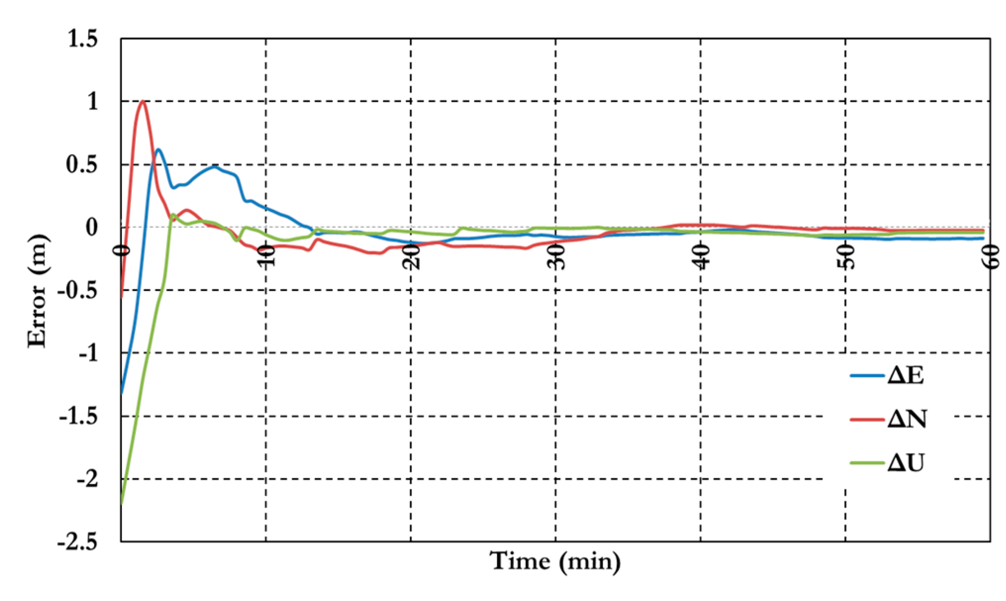
Figure 7 and
Figure 8 show the positioning results and the estimated ambiguity parameters of the traditional PPP model using GPS/Galileo observations.
Figure 7.
Postioining results of the traditional GPS/Galileo PPP model.
Figure 7.
Postioining results of the traditional GPS/Galileo PPP model.
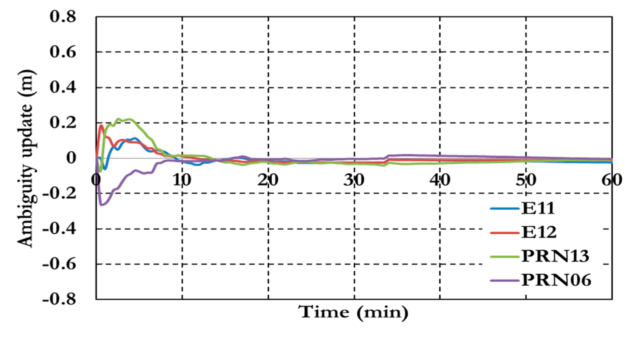
Figure 8.
Ambiguity parameters the traditional GPS/Galileo PPP model.
Figure 8.
Ambiguity parameters the traditional GPS/Galileo PPP model.
As shown in
Figure 6, the positioning results of the combined GPS/Galileo traditional PPP model have a convergence time of 15 min to reach decimeter-level precision. The ambiguity parameters results in
Figure 8 shows that the un-calibrated hardware delayed that lumped to the ambiguity parameter affects the ambiguity parameters convergence.
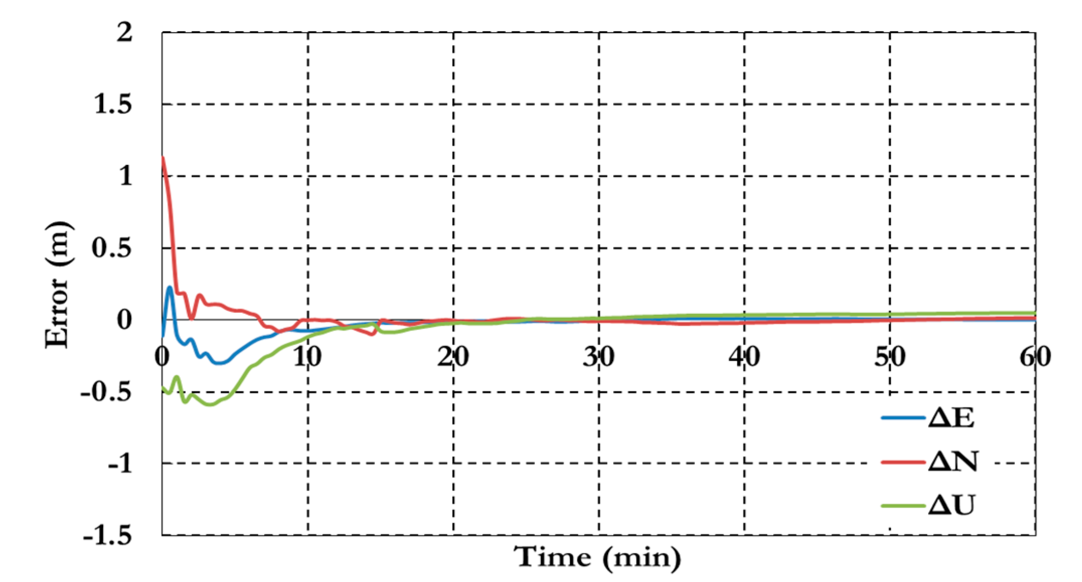
Figure 9,
Figure 10 and
Figure 11 show the results of the GPS decoupled clock model.
Figure 9.
Positioning results of the GPS decoupled clock model.
Figure 9.
Positioning results of the GPS decoupled clock model.
Figure 9 shows the positioning results of the decoupled clock model. The results show a decimeter level of precision with about 15 min. Generally the precision of the decoupled clock model positioning results are about 25% more than the traditional PPP model.
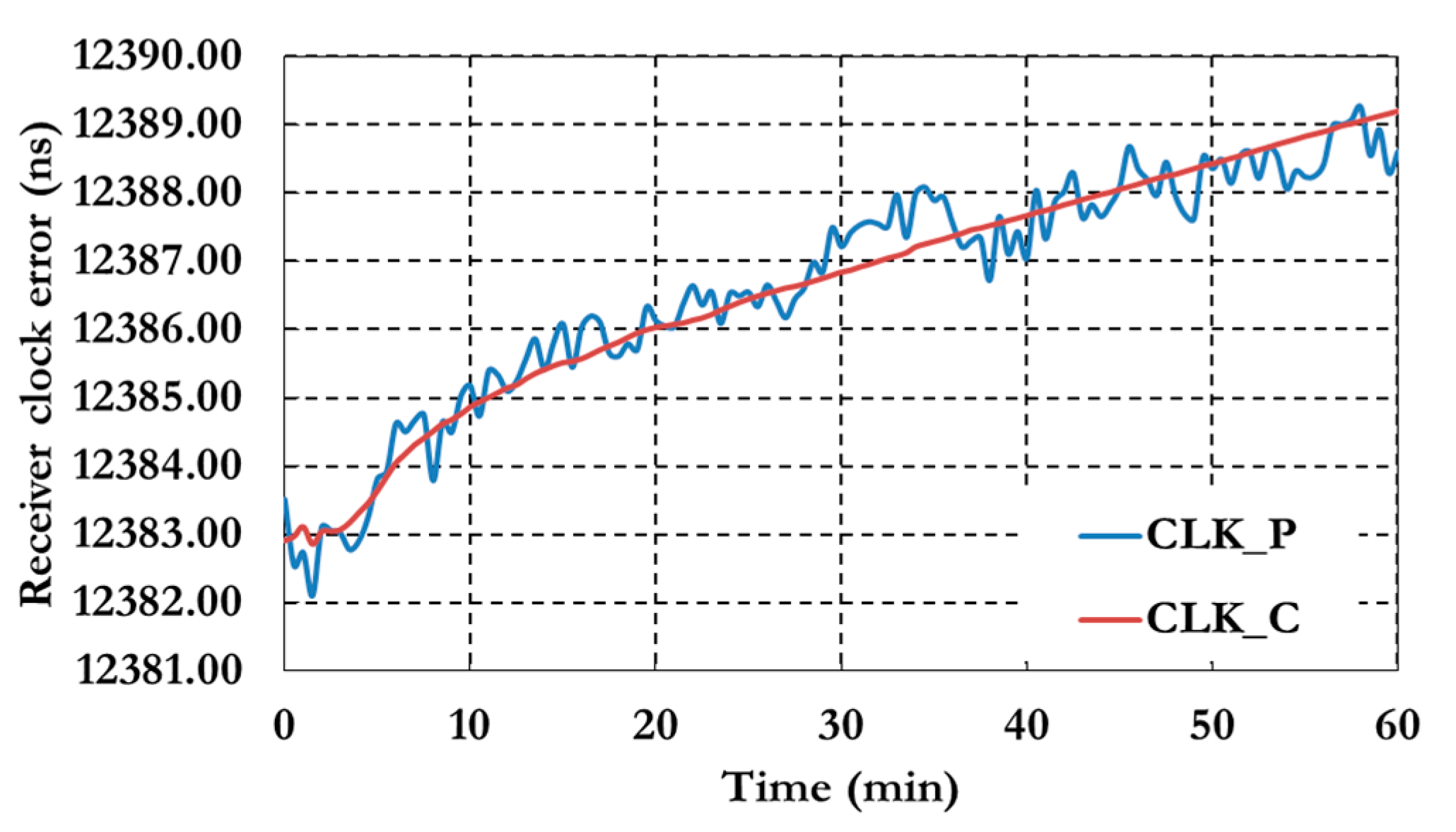
Figure 10 shows the receiver clock errors for both pseudorange (CLK_P) and carrier phase (CLK_C) observation.
Figure 10.
Receiver clock errors of the GPS decoupled clock model.
Figure 10.
Receiver clock errors of the GPS decoupled clock model.
Figure 11 shows the results of the ambiguity parameters of the GPS decoupled clock model.
Figure 11.
Ambiguity parameters of the GPS decoupled clock model.
Figure 11.
Ambiguity parameters of the GPS decoupled clock model.
Figure 12,
Figure 13,
Figure 14 and
Figure 15 show the results of the semi-decoupled clock GPS/Galileo PPP model. The positioning results in
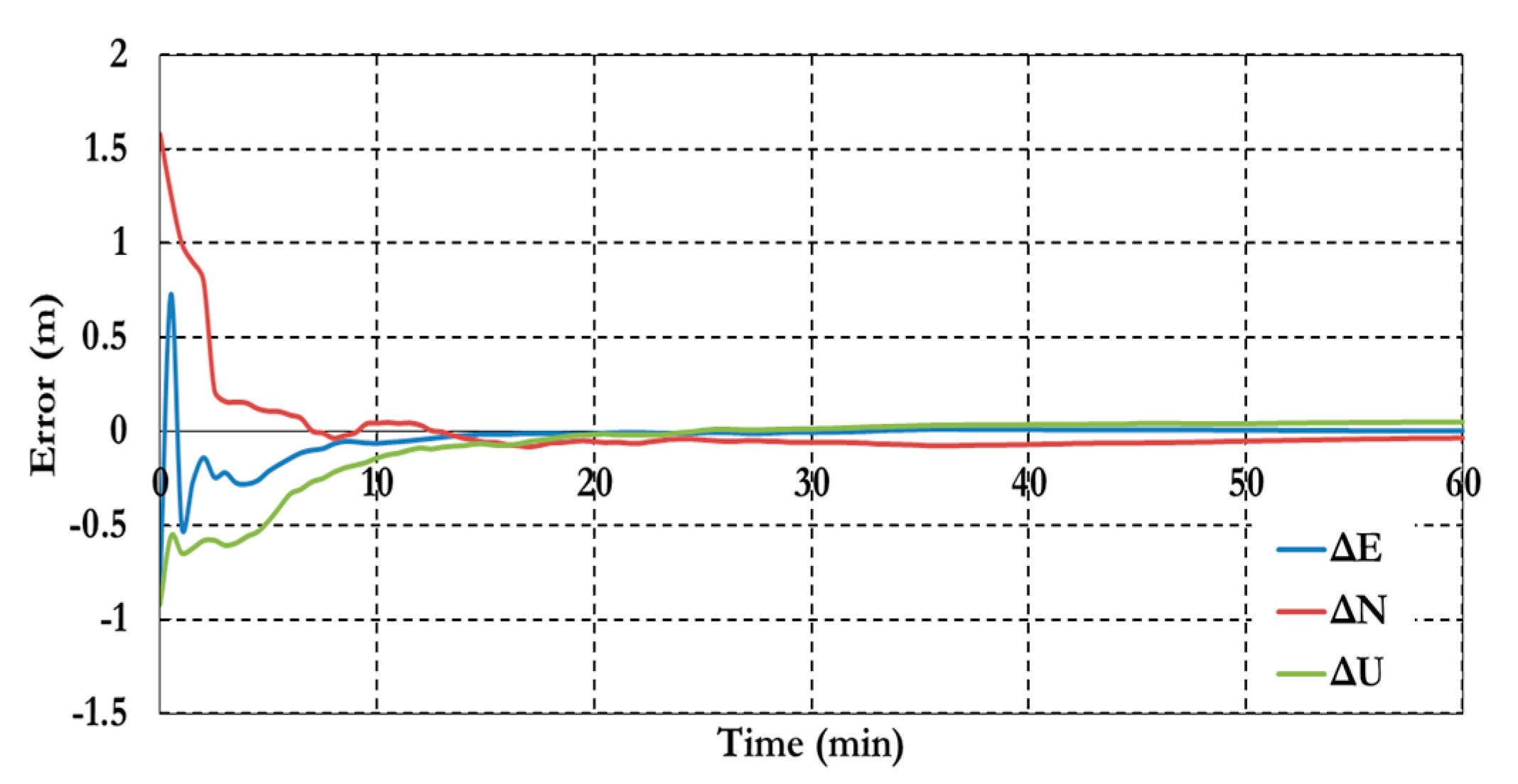
Figure 16 show that the semi-decoupled clock GPS/Galileo PPP model has a decimeter level of precision with about 15 min. In addition, the positioning precision of the semi-decoupled clock GPS/Galileo PPP model are improved by about 25% comparing to the traditional GPS/Galileo PPP model.
Figure 12.
Positioning results of the semi-decoupled clock PPP model.
Figure 12.
Positioning results of the semi-decoupled clock PPP model.
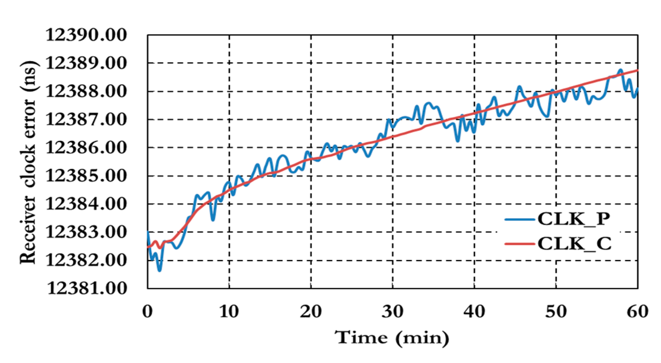
Figure 13 shows the receiver clock errors for both pseudorange (CLK_P) and carrier phase (CLK_C) observation.
Figure 13.
Receiver clock errors of the semi-decoupled clock GPS/Galileo PPP model.
Figure 13.
Receiver clock errors of the semi-decoupled clock GPS/Galileo PPP model.
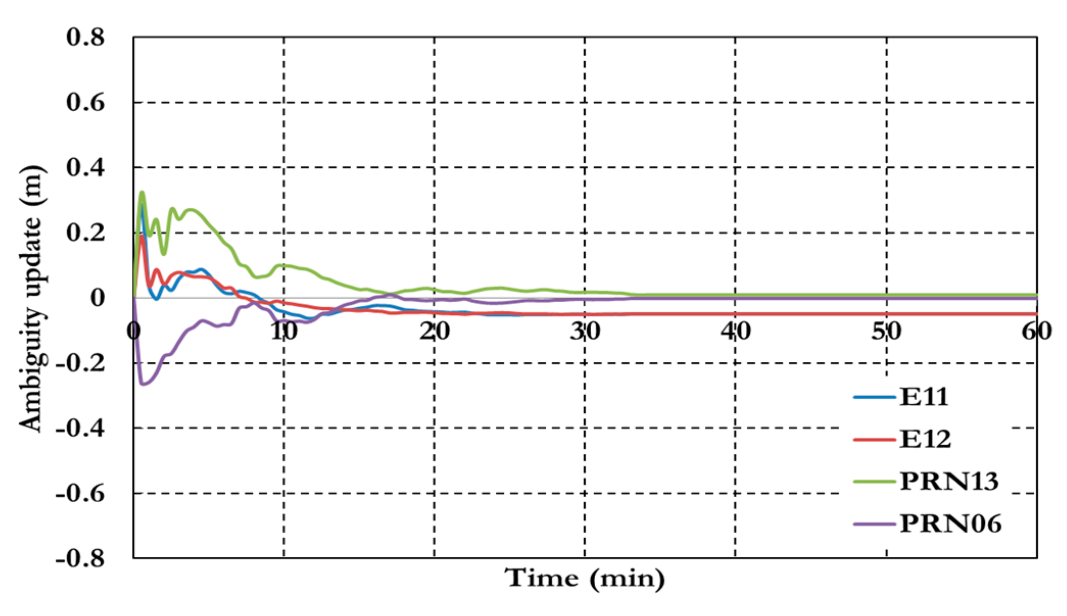
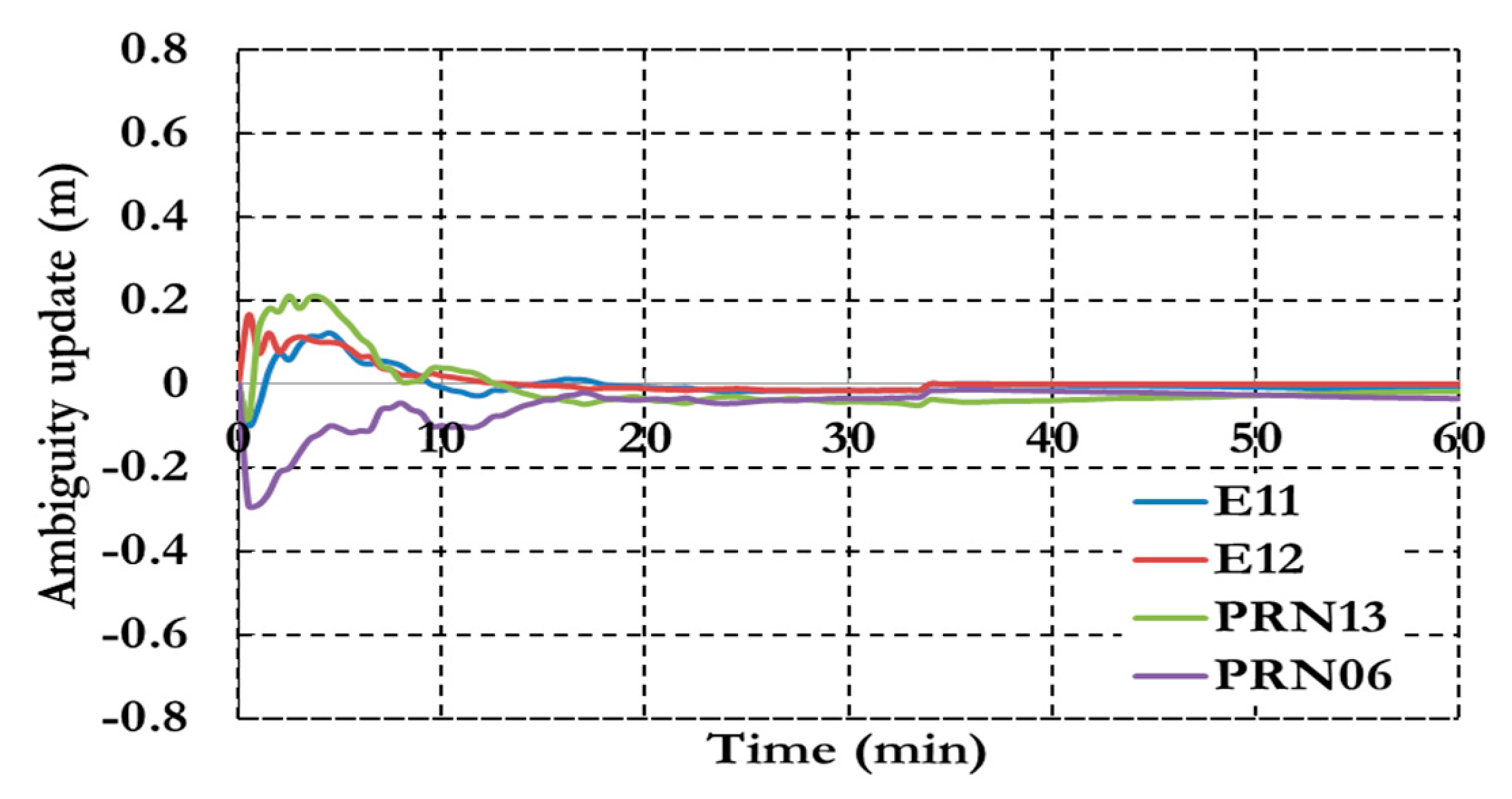
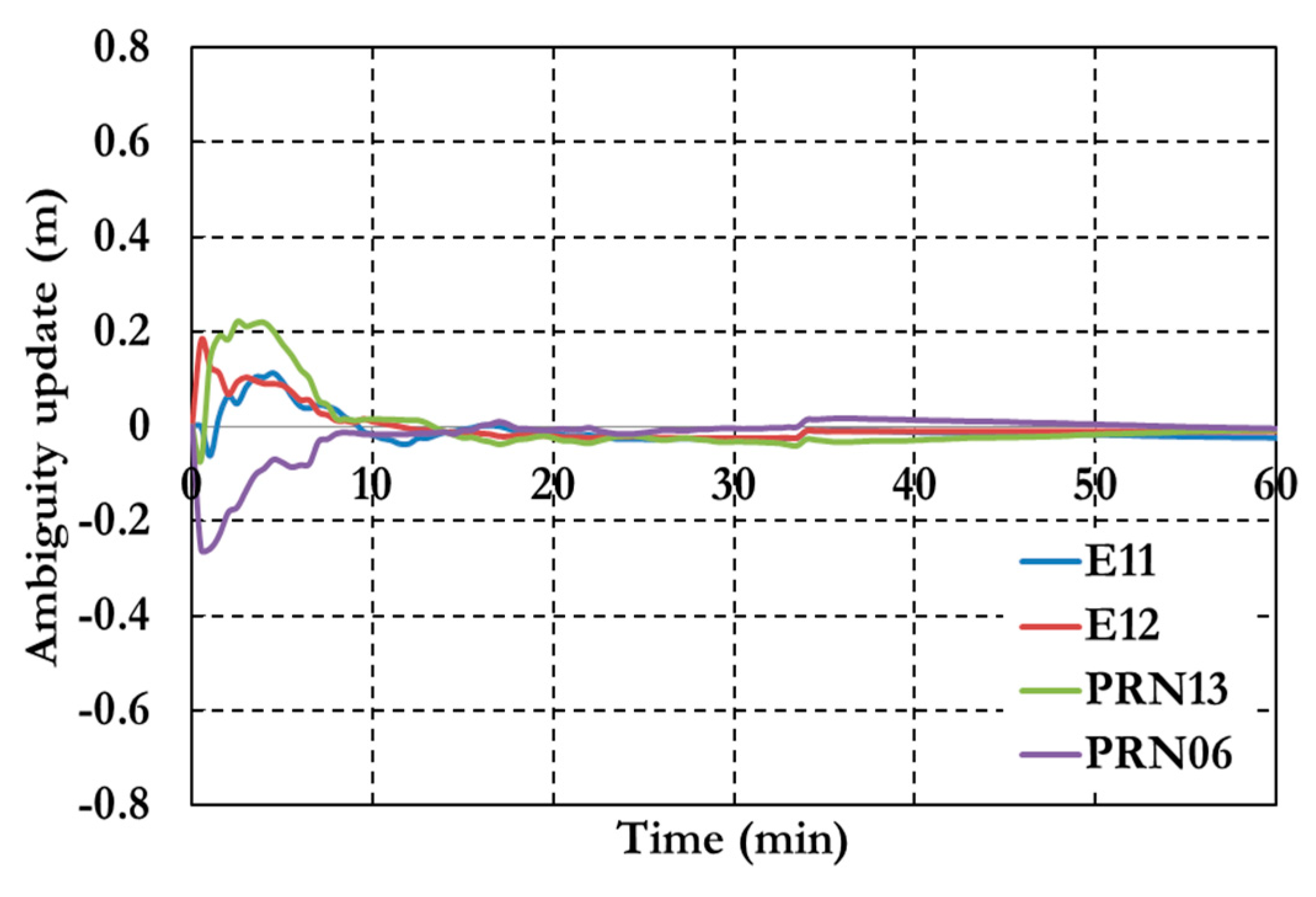
Figure 14 shows the ambiguity parameters results of the semi-decoupled clock GPS/Galileo PPP model.
Figure 14.
Ambiguity parameters of the semi-decoupled clock GPS/Galileo PPP model.
Figure 14.
Ambiguity parameters of the semi-decoupled clock GPS/Galileo PPP model.
As shown in
Figure 14 the ambiguity parameters results show a similar convergence time to the positioning results.
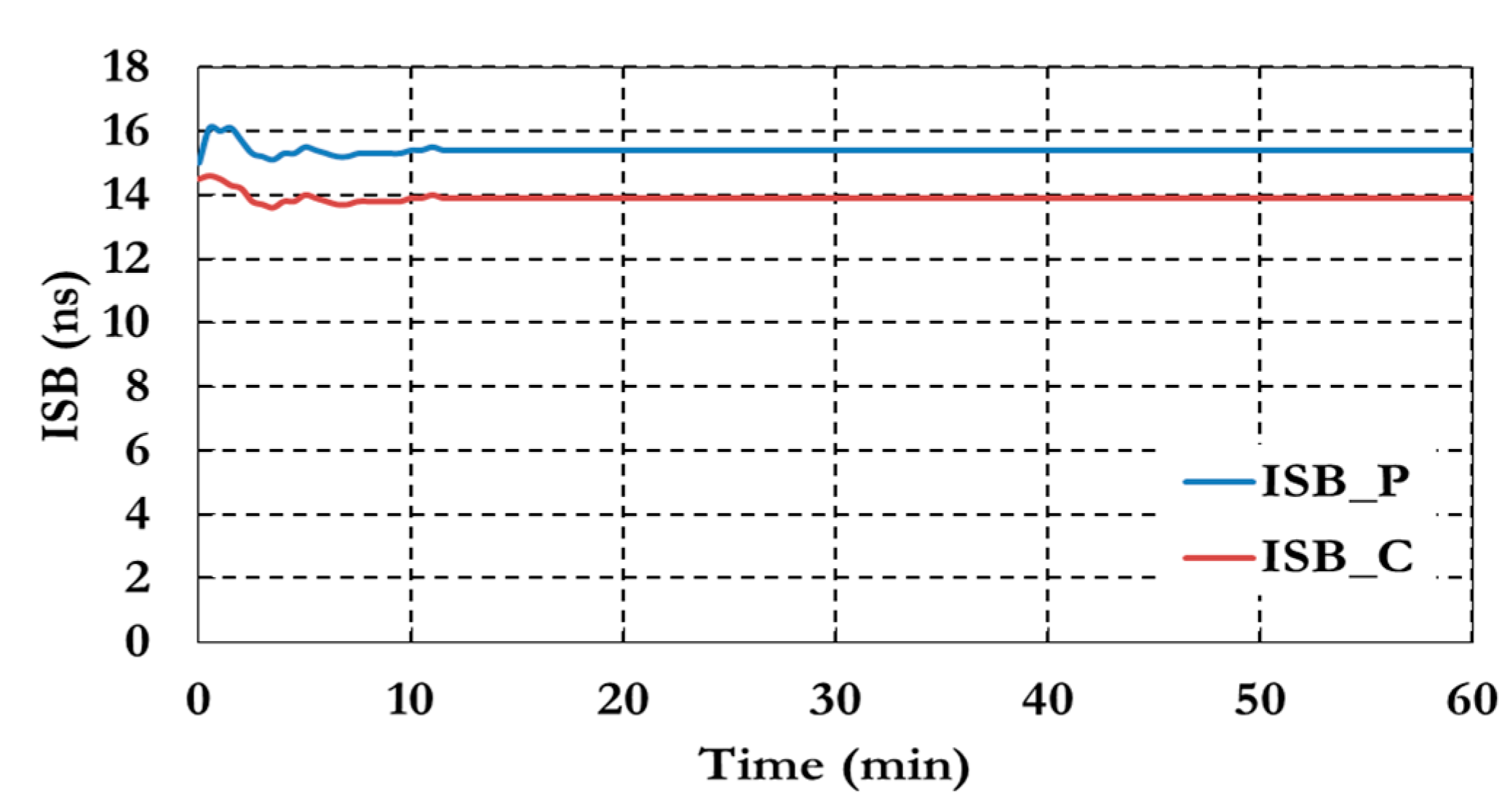
Figure 15 shows the results of the inter-system bias parameters for both pseudorange (ISB_P) and carrier phase (ISB_C) observations.
Figure 15.
Inter-system bias of the semi-decoupled clock GPS/Galileo PPP model.
Figure 15.
Inter-system bias of the semi-decoupled clock GPS/Galileo PPP model.
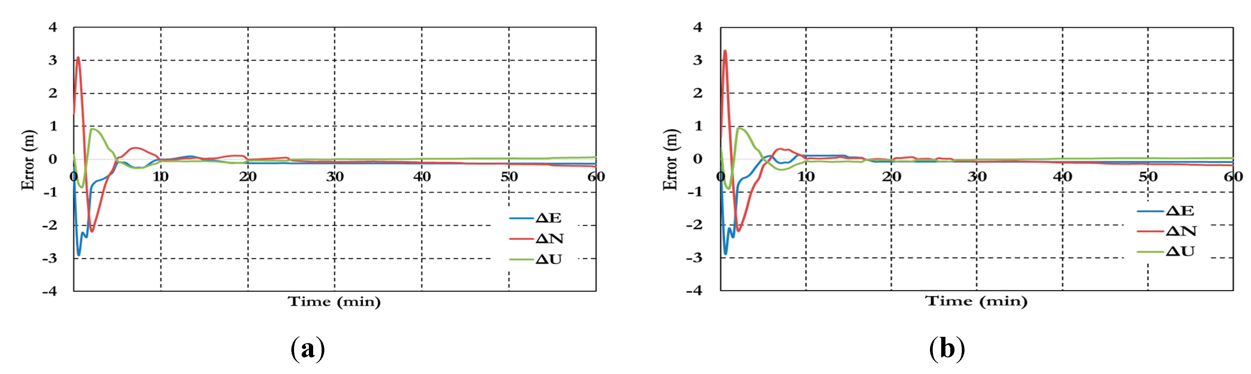
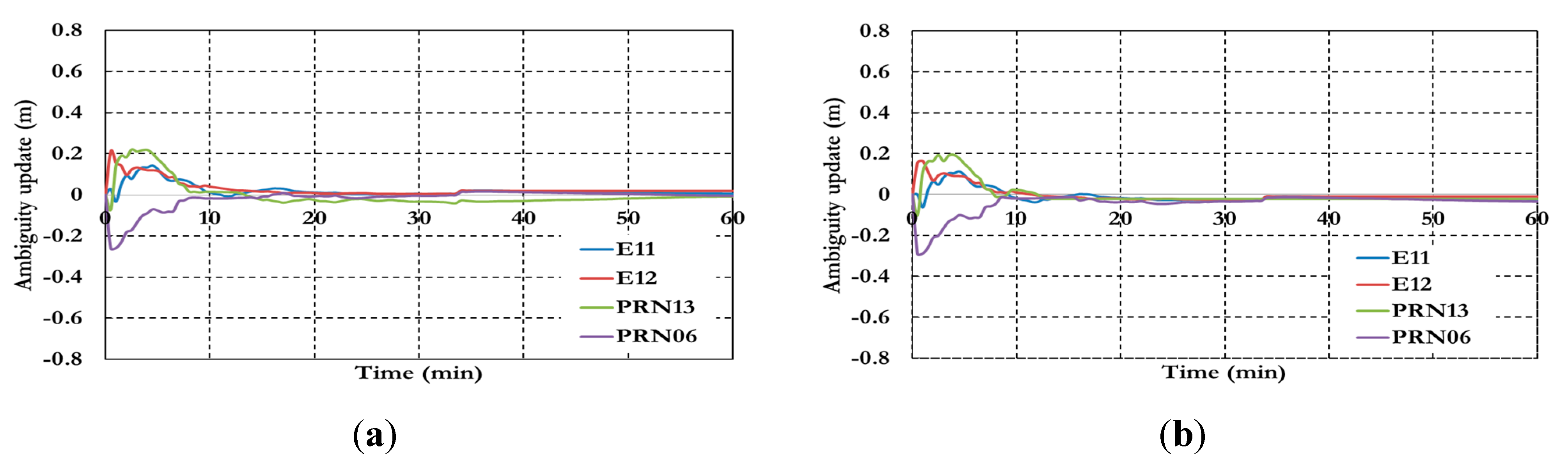
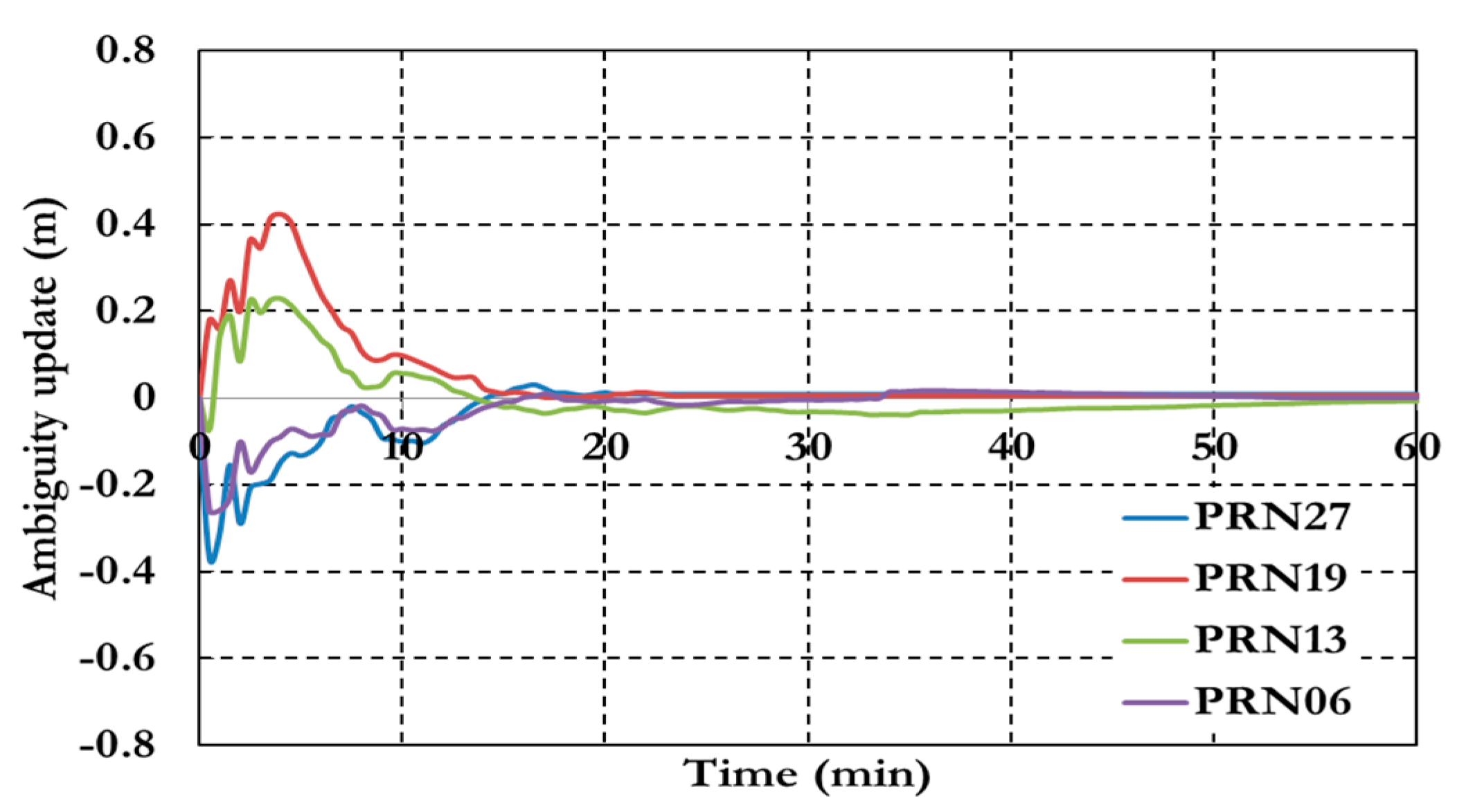
Figure 16 and
Figure 17 show the BSSD PPP tight combination model positioning results and the estimated ambiguity parameters.
Figure 16.
Positioning results of the BSSD PPP tight combination model using (a) GPS reference satellite; and (b) Galileo reference satellite
Figure 16.
Positioning results of the BSSD PPP tight combination model using (a) GPS reference satellite; and (b) Galileo reference satellite
As shown in
Figure 16, the positioning results of the BSSD tight combination model have convergence time of 10 min and decimeter level of precision.
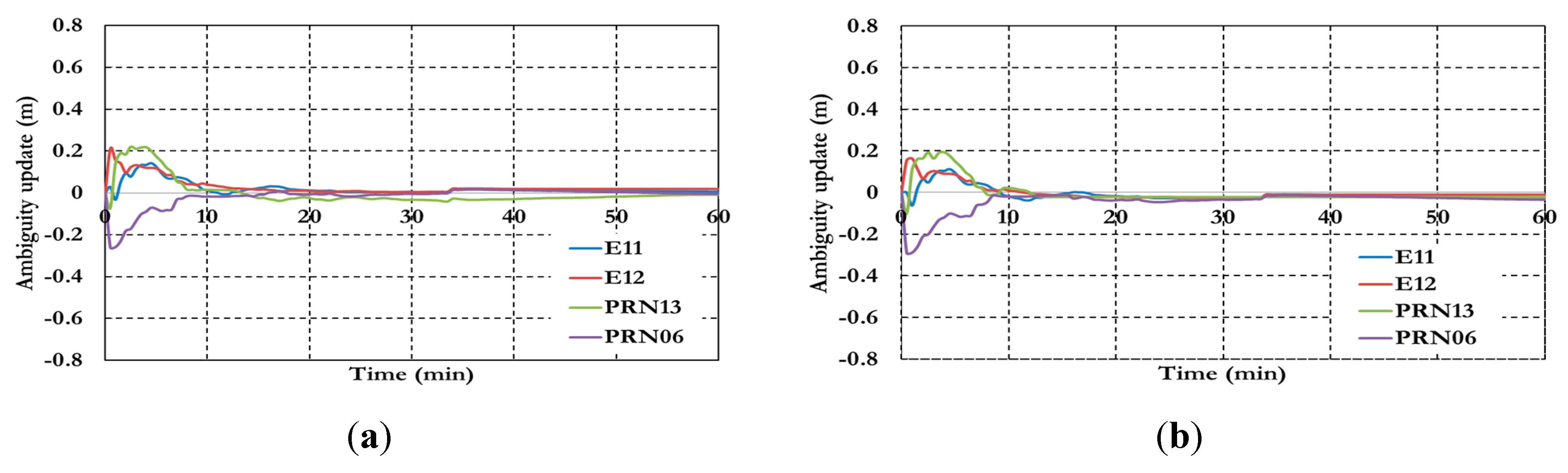
Figure 17.
Ambiguity parameters the BSSD PPP tight combination model using (a) GPS reference satellite; and (b) Galileo reference satellite.
Figure 17.
Ambiguity parameters the BSSD PPP tight combination model using (a) GPS reference satellite; and (b) Galileo reference satellite.
As shown in
Figure 17, the results convergence of the ambiguity parameters are affected by the lumped DCB.
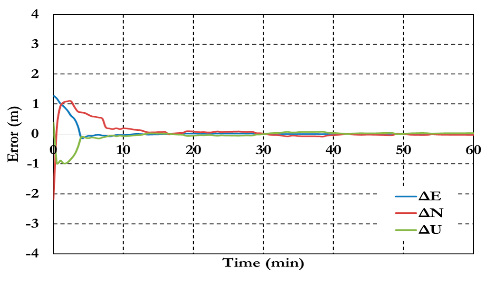
Figure 18 and
Figure 19 show the results of the BSSD PPP loose combination model for both positioning results and ambiguity parameters.
Figure 18.
Positioning results of the BSSD PPP loose combination model.
Figure 18.
Positioning results of the BSSD PPP loose combination model.
Figure 19.
Ambiguity parameters the BSSD PPP loose combination model.
Figure 19.
Ambiguity parameters the BSSD PPP loose combination model.
As shown in
Figure 18, the positioning results show decimeter-level precision with about 11 min convergence time.
Figure 19 shows that the ambiguity parameters of the BSSD loose combination model are affected by the lumped DCB.
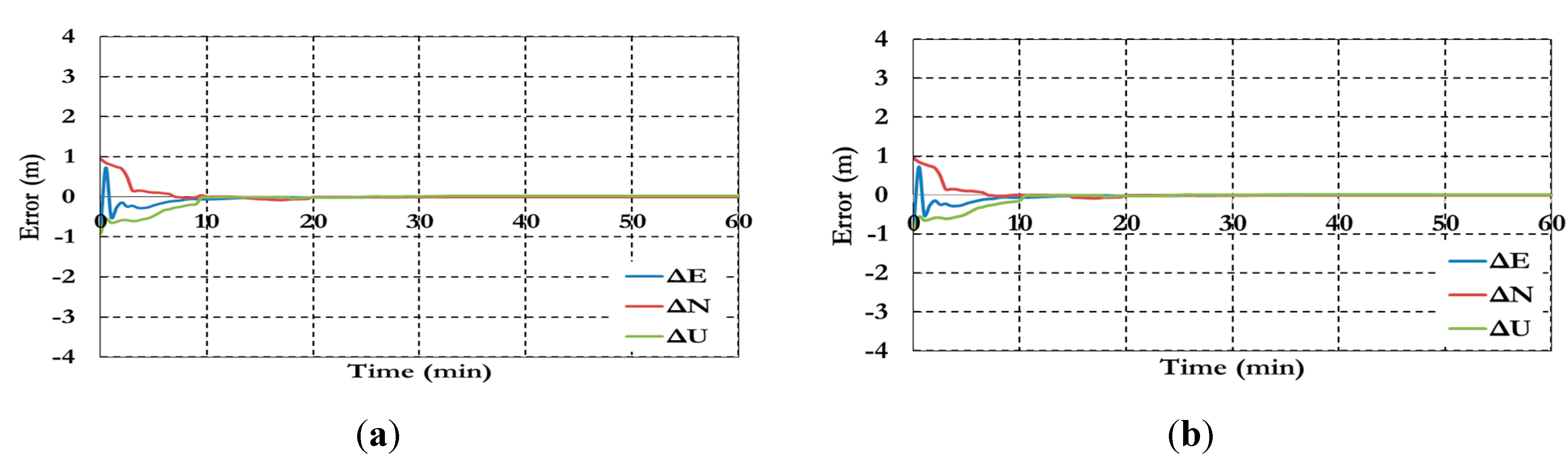
Figure 20 and
Figure 21 show the positioning results and the estimated ambiguity parameters for the BSSD semi-decoupled GPS/Galileo PPP model, when a tight combination is used. As can be seen, the PPP solution convergences to a decimeter-level precision after about 10 min.
Figure 20.
Positioning results for BSSD semi-decoupled GPS/Galileo PPP model. (a) GPS reference satellite; and (b) Galileo reference satellite.
Figure 20.
Positioning results for BSSD semi-decoupled GPS/Galileo PPP model. (a) GPS reference satellite; and (b) Galileo reference satellite.
Figure 21.
Ambiguity parameters the semi-decoupled GPS/Galileo PPP model (a) GPS reference satellite; and (b) Galileo reference satellite.
Figure 21.
Ambiguity parameters the semi-decoupled GPS/Galileo PPP model (a) GPS reference satellite; and (b) Galileo reference satellite.
Figure 22 and
Figure 23 show the results of the semi-decoupled per-constellation GPS/Galileo BSSD PPP model for both of the positioning and ambiguity parameters. As can be seen, the positioning results show decimeter-level precision with about 11 min convergence time.
Figure 22.
Positioning results of the semi-decoupled per-constellation GPS/Galileo BSSD PPP model.
Figure 22.
Positioning results of the semi-decoupled per-constellation GPS/Galileo BSSD PPP model.
Figure 23.
Ambiguity parameters the semi-decoupled per-constellation GPS/Galileo BSSD PPP model.
Figure 23.
Ambiguity parameters the semi-decoupled per-constellation GPS/Galileo BSSD PPP model.
As shown in
Figure 23, the ambiguity parameters results for both GPS and Galileo satellites are affected by the lumped DCB.
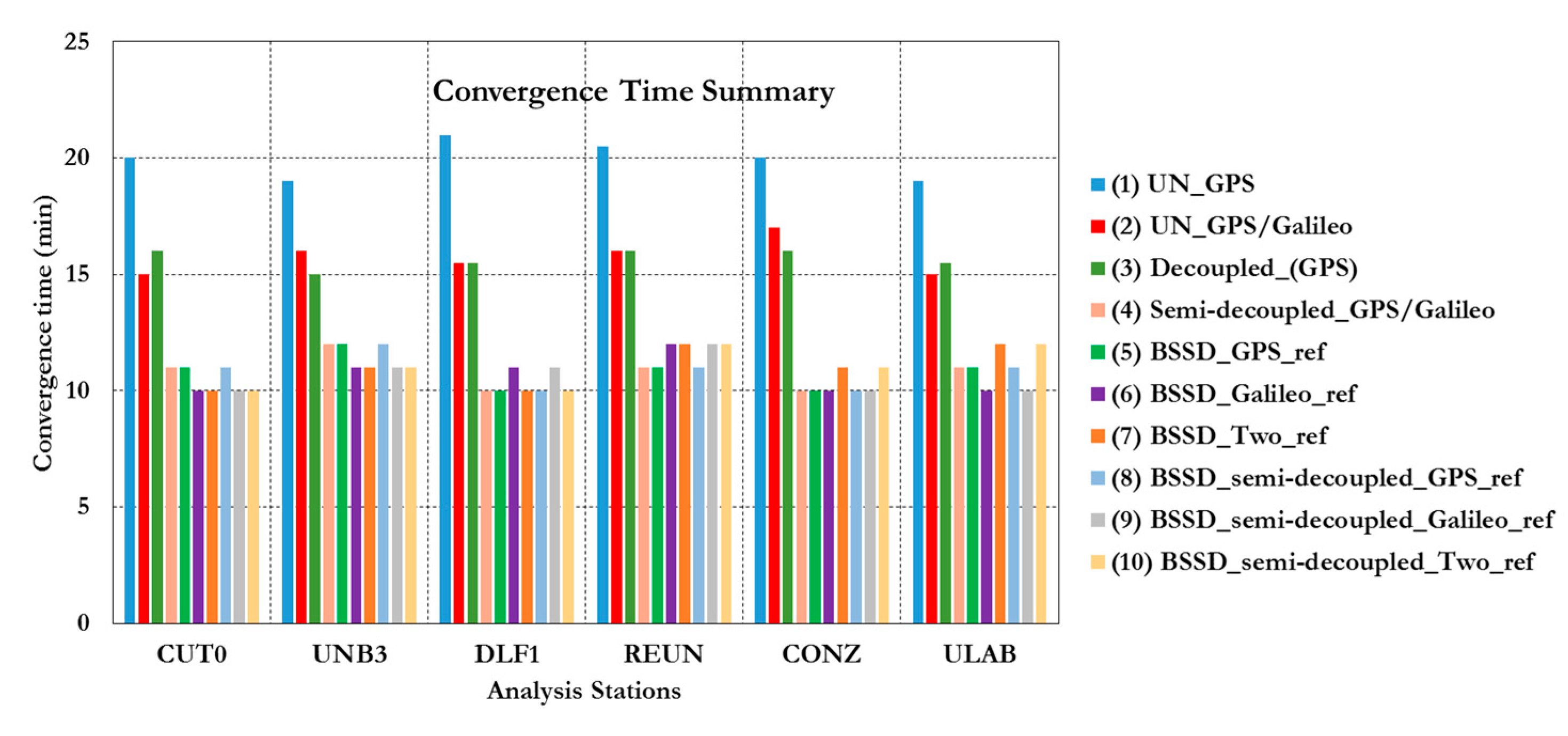
Figure 24 summarizes the convergence times for all analysis cases, which confirm the PPP solution consistency at all stations.
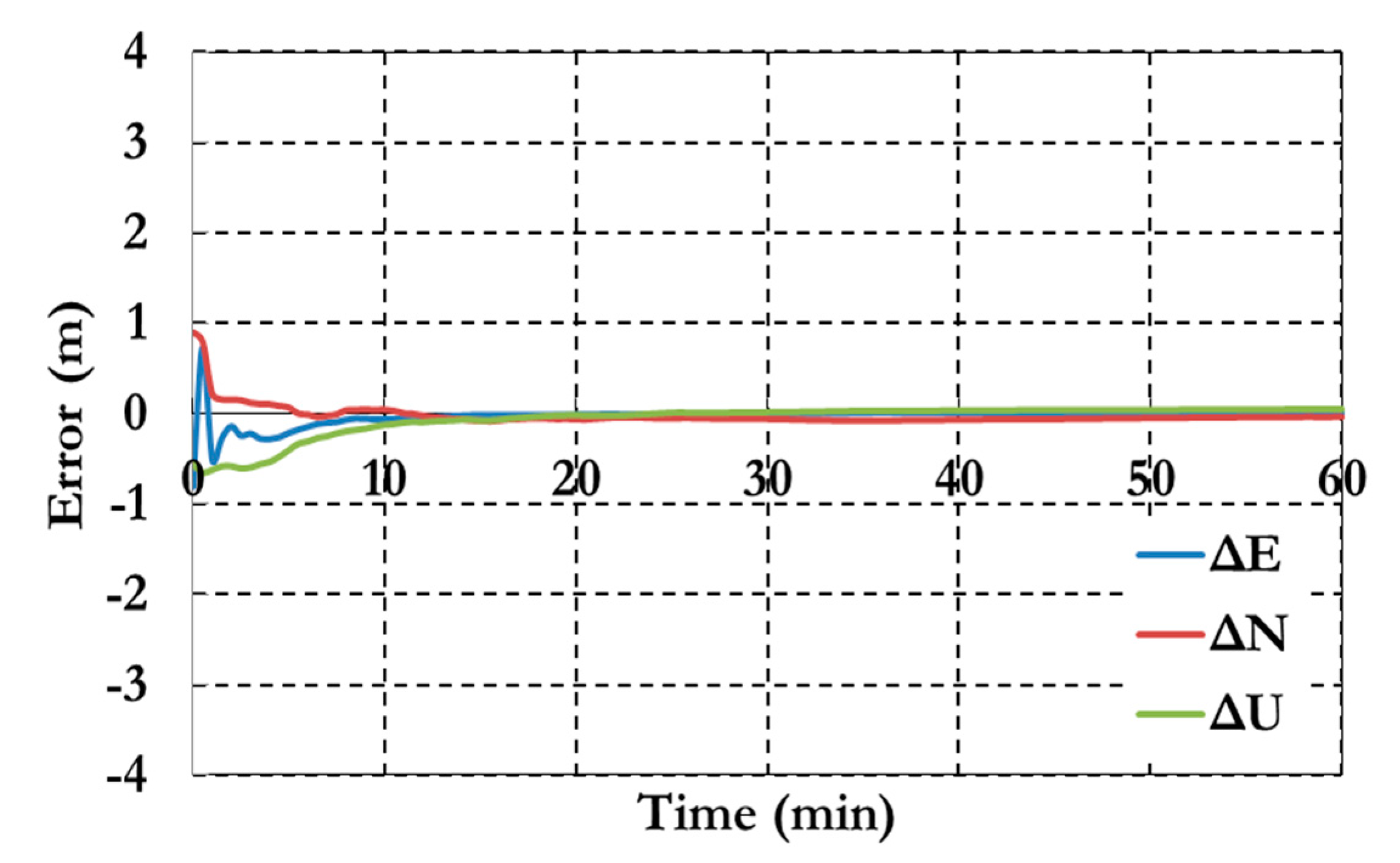
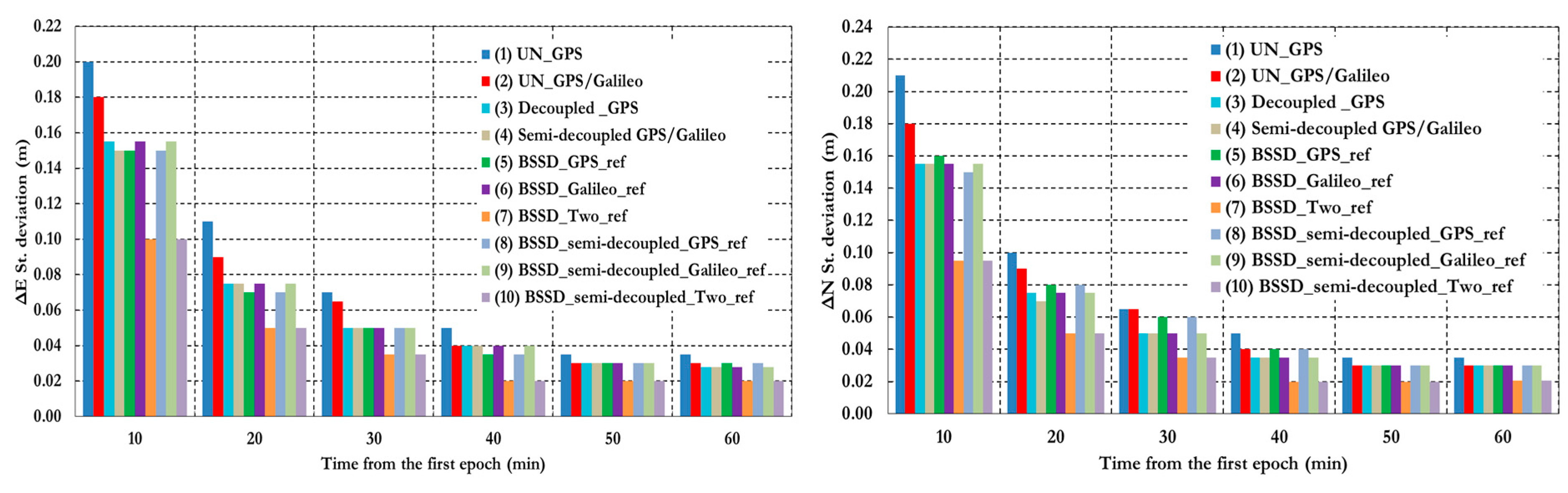
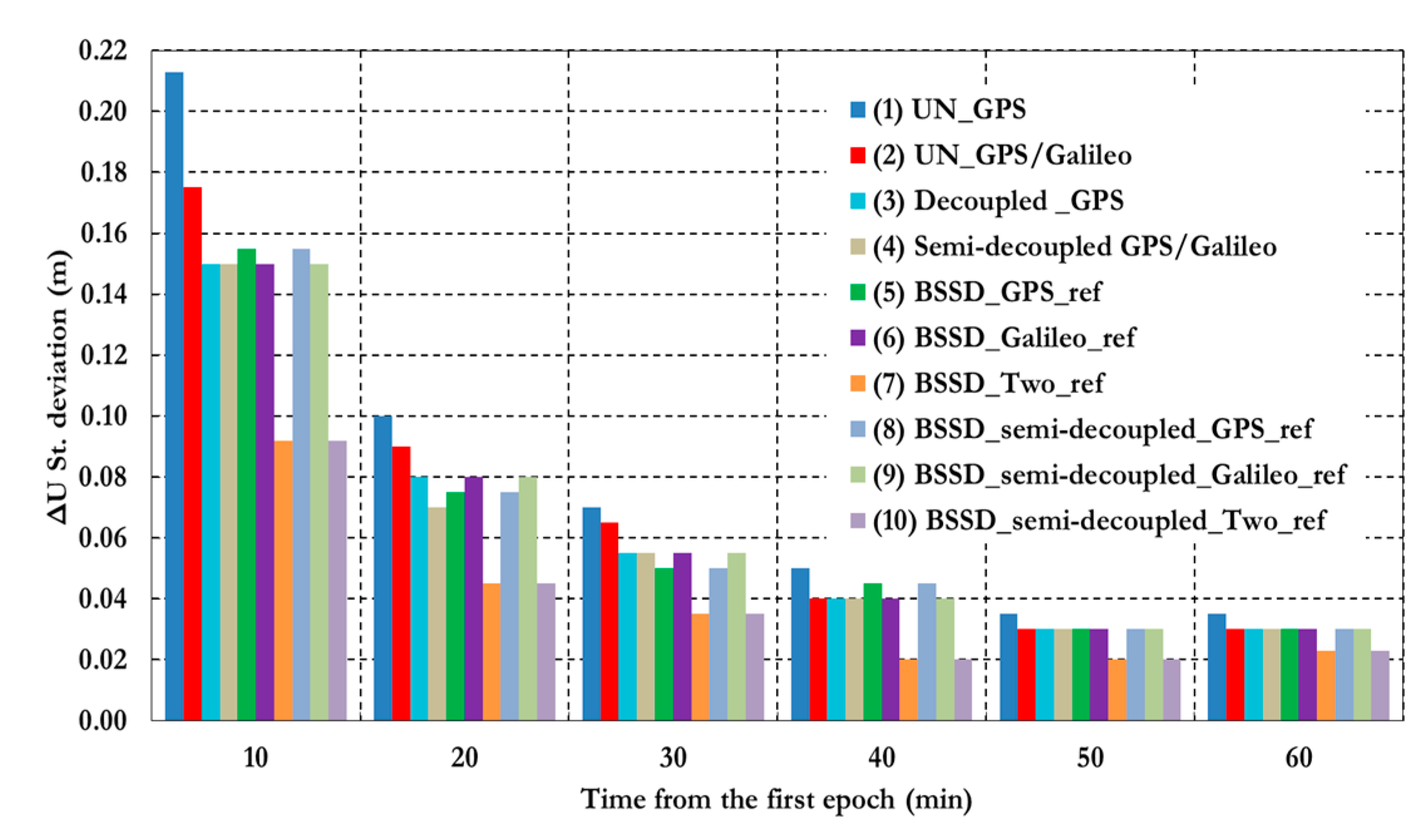
To further assess the performance of the various PPP models, the solution output is sampled every 10 min and the standard deviation of the computed station coordinates is calculated for each sample.
Figure 25 shows the position standard deviations in the East, North, and Up directions, respectively. Examining the standard deviations after 10 min, it can be seen that the semi-decoupled clock GPS/Galileo PPP model improves the precision of the estimated parameters by about 25% in comparison with the un-differenced GPS-only model. As the number of epochs, and consequently the number of measurements, increases the performance of the various models tends to be comparable. An exception, however, is the loose combination model, which is found superior to all other PPP models.
Figure 24.
Summary of convergence times of all stations and analysis cases. (1) Un-differenced GPS model; (2) Un-differenced GPS/Galileo model; (3) Decoupled clock model using GPS observations only; (4) semi-decoupled clock GPS/Galileo PPP model; (5) BSSD model with a GPS satellite as a reference; (6) BSSD model with a Galileo satellite as a reference; (7) BSSD model with both a GPS and a Galileo satellite as reference satellites; (8) BSSD semi-decoupled clock GPS/Galileo model with a GPS satellite as a reference; (9) BSSD semi-decoupled clock GPS/Galileo model with a Galileo satellite as a reference; (10) BSSD semi-decoupled clock GPS/Galileo model with both a GPS and a Galileo satellite as reference satellites.
Figure 25.
Summary of positioning standard deviations in East, North, and Up directions of all stations and analysis cases. (1) Un-differenced GPS model; (2) Un-differenced GPS/Galileo model; (3) Decoupled clock model using GPS observations only; (4) semi-decoupled clock GPS/Galileo PPP model; (5) BSSD model with a GPS satellite as a reference; (6) BSSD model with a Galileo satellite as a reference; (7) BSSD model with both a GPS and a Galileo satellite as reference satellites; (8) BSSD semi-decoupled clock GPS/Galileo model with a GPS satellite as a reference; (9) BSSD semi-decoupled clock GPS/Galileo model with a Galileo satellite as a reference; (10) BSSD semi-decoupled clock GPS/Galileo model with both a GPS and a Galileo satellite as reference satellites.


