
Tracking Multiple Video Targets with an Improved GM-PHD Tracker


Abstract
:1. Introduction

2. Problem Formulation
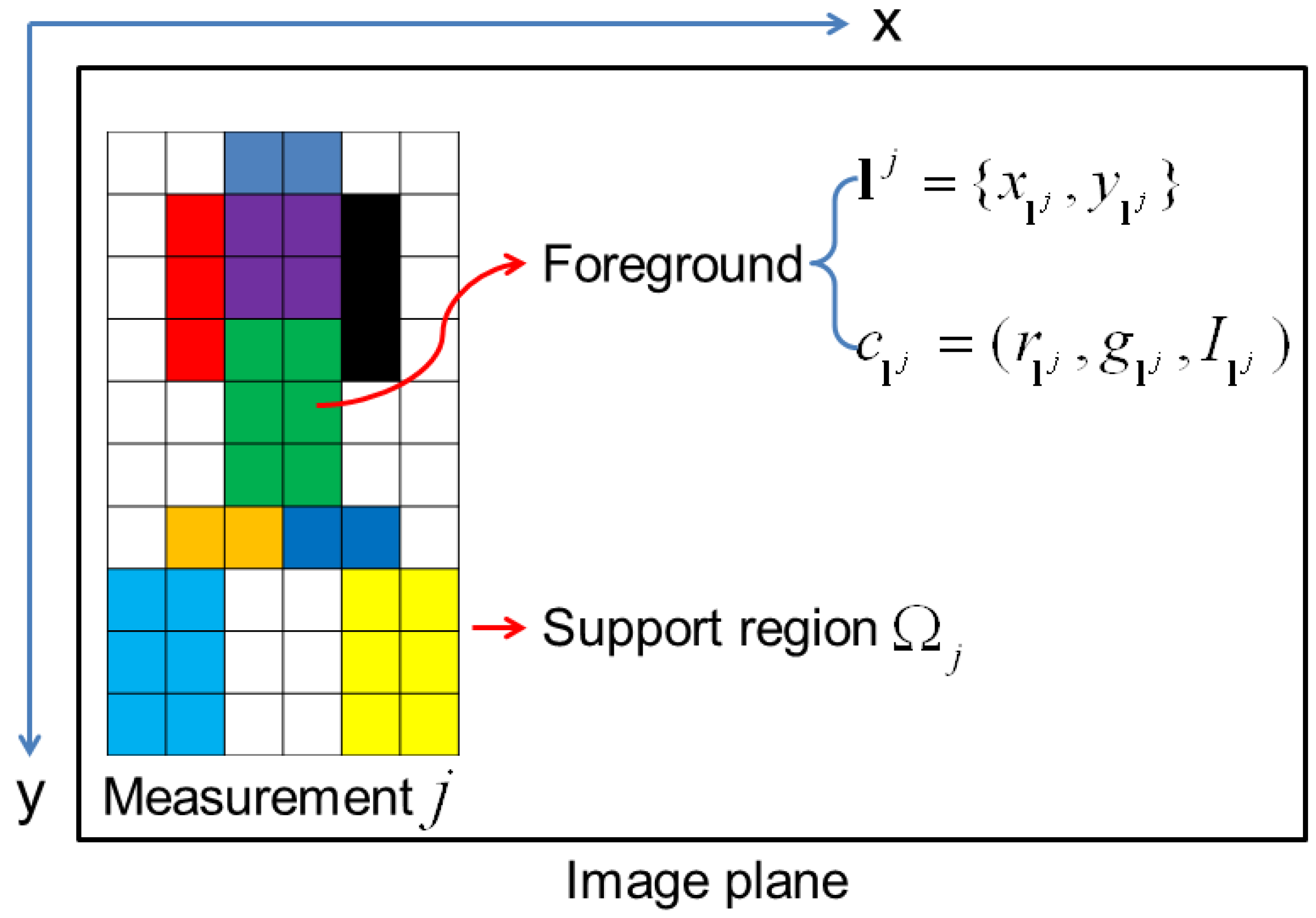
2.1. Target State and Measurement Representation
2.2. The GM-PHD Filter
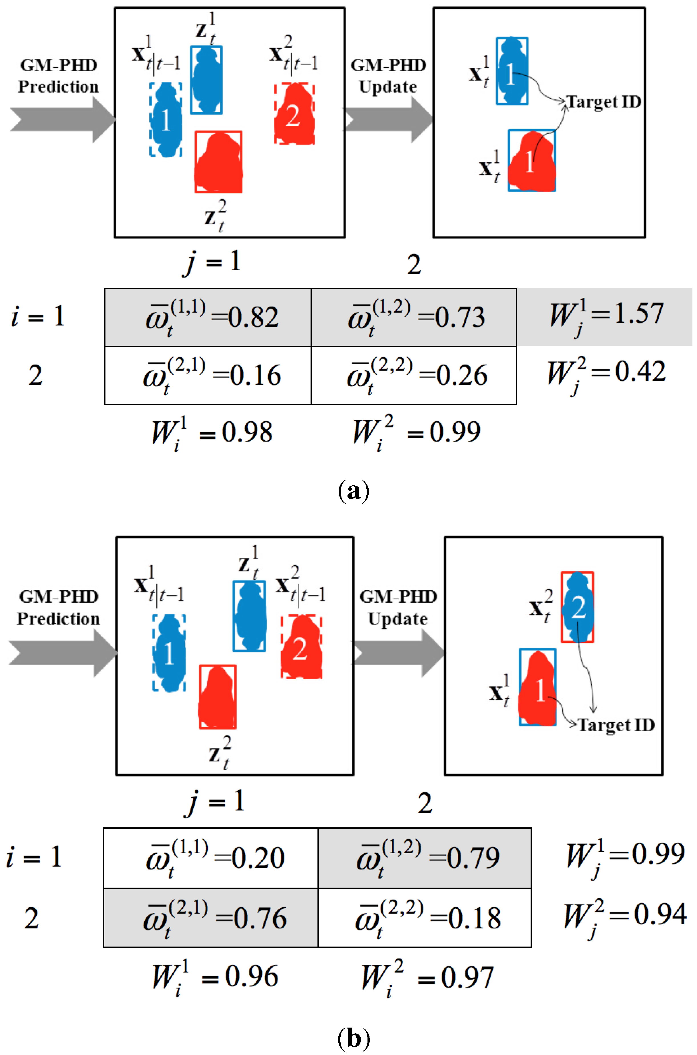
2.3. Drawbacks of the GM-PHD Filter
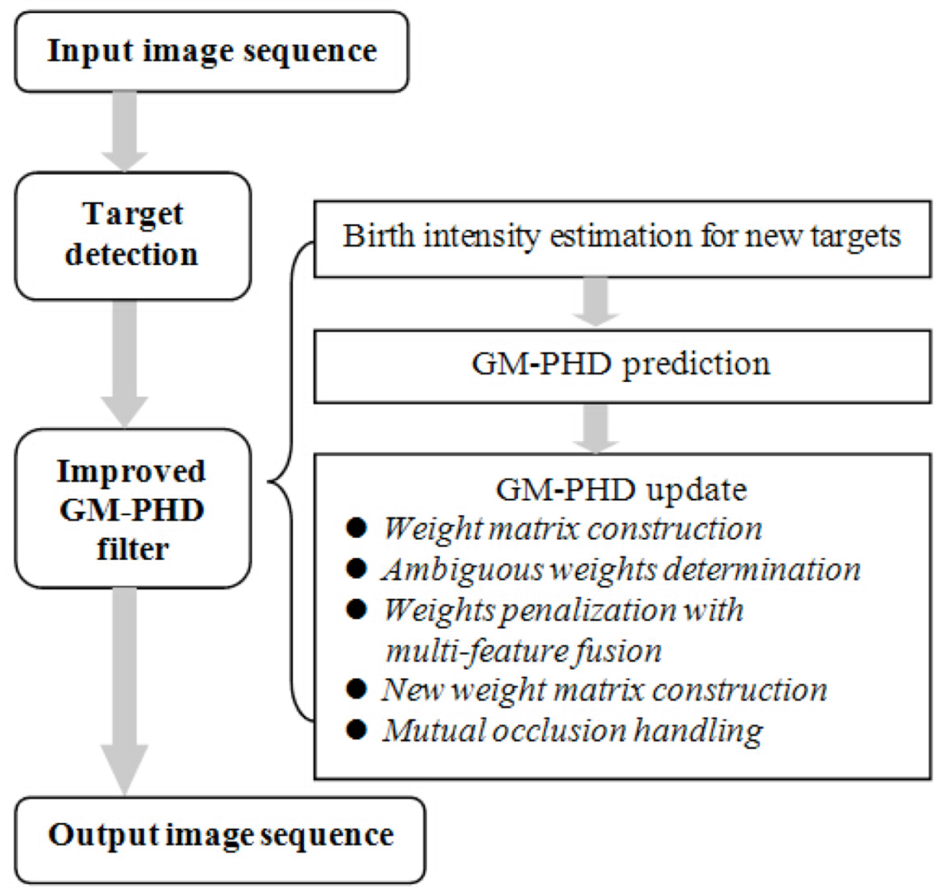
3. Improved GM-PHD Tracker with Weight Penalization
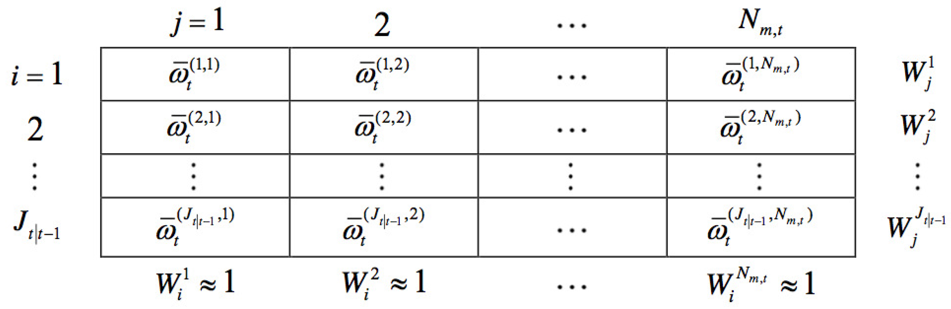
3.1. Weight Matrix Construction

3.2. Ambiguous Weight Determination
3.3. Multi-Feature Fusion
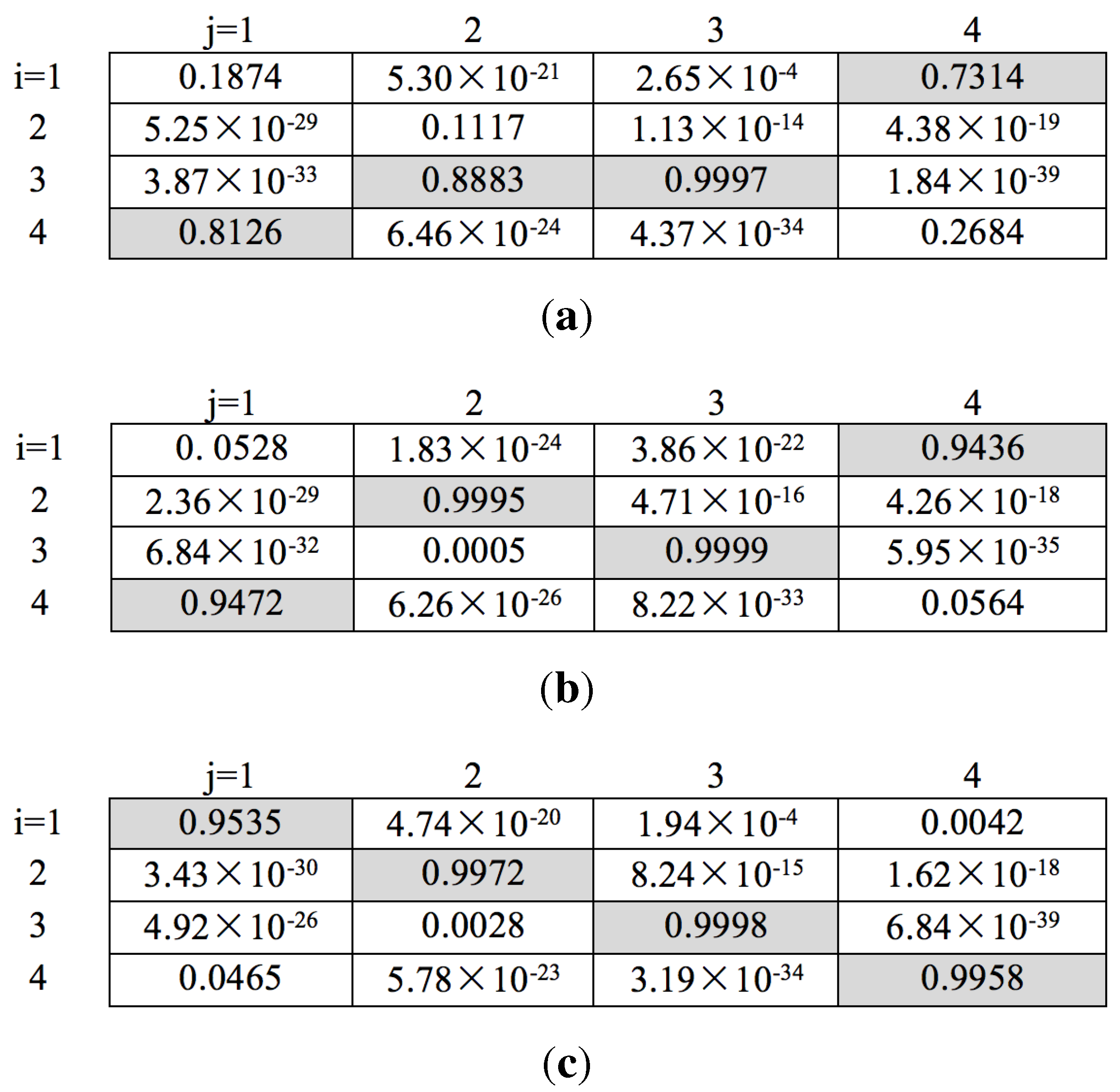
3.4. Weight Penalization
4. Experimental Evaluation
4.1. Experimental Parameter Setup
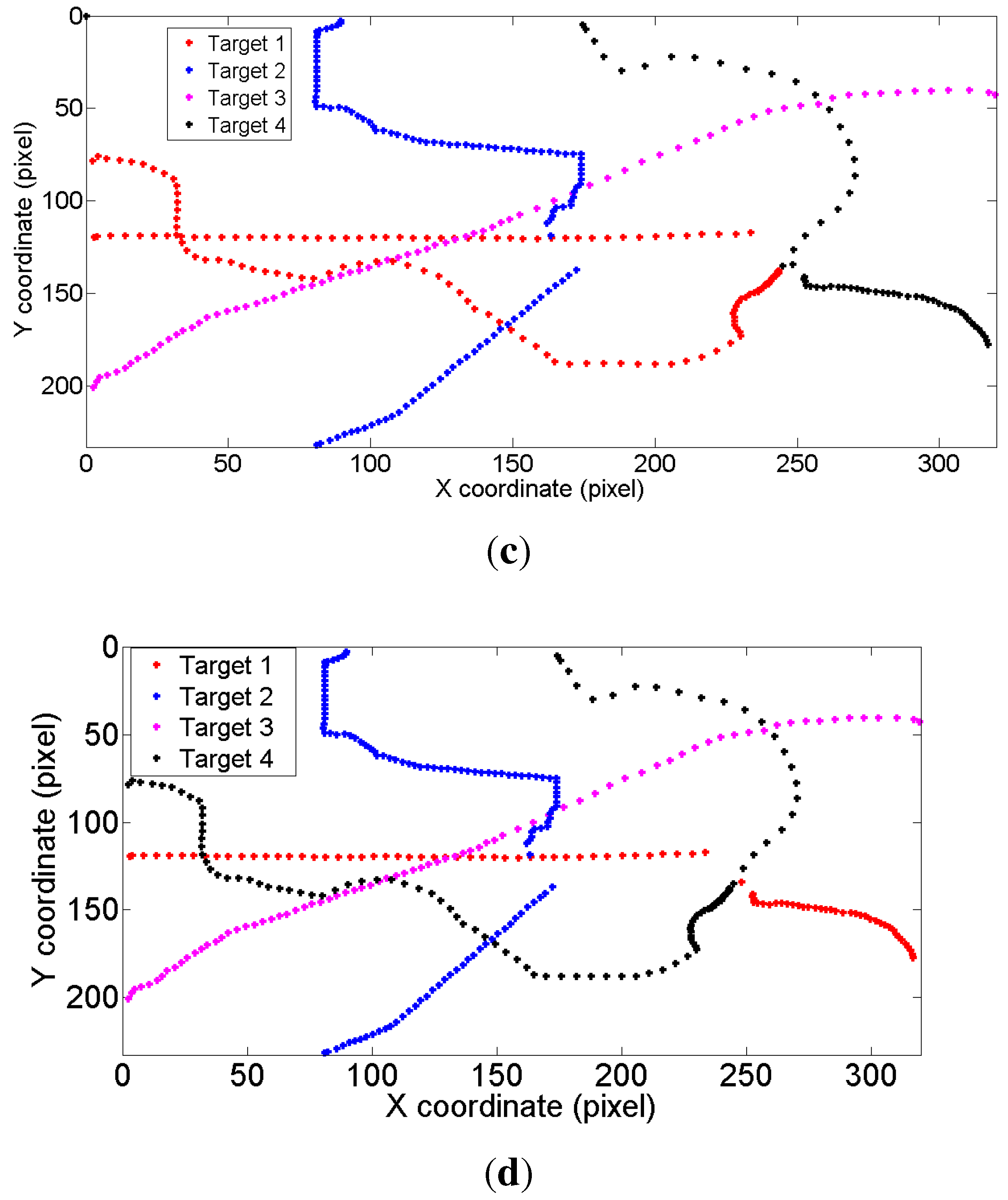
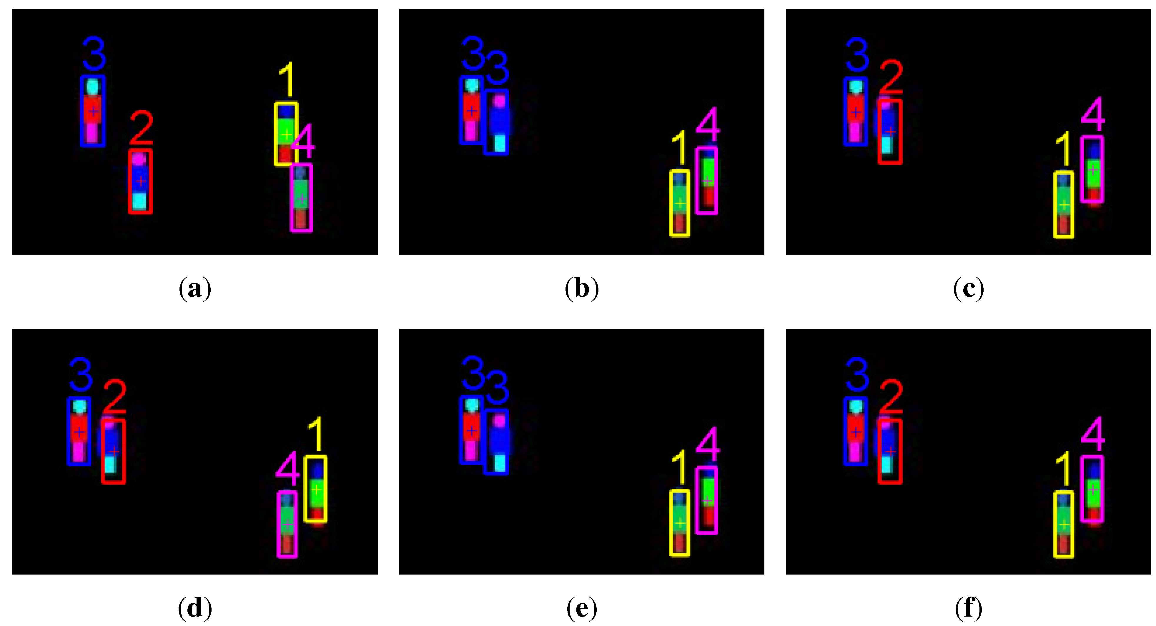
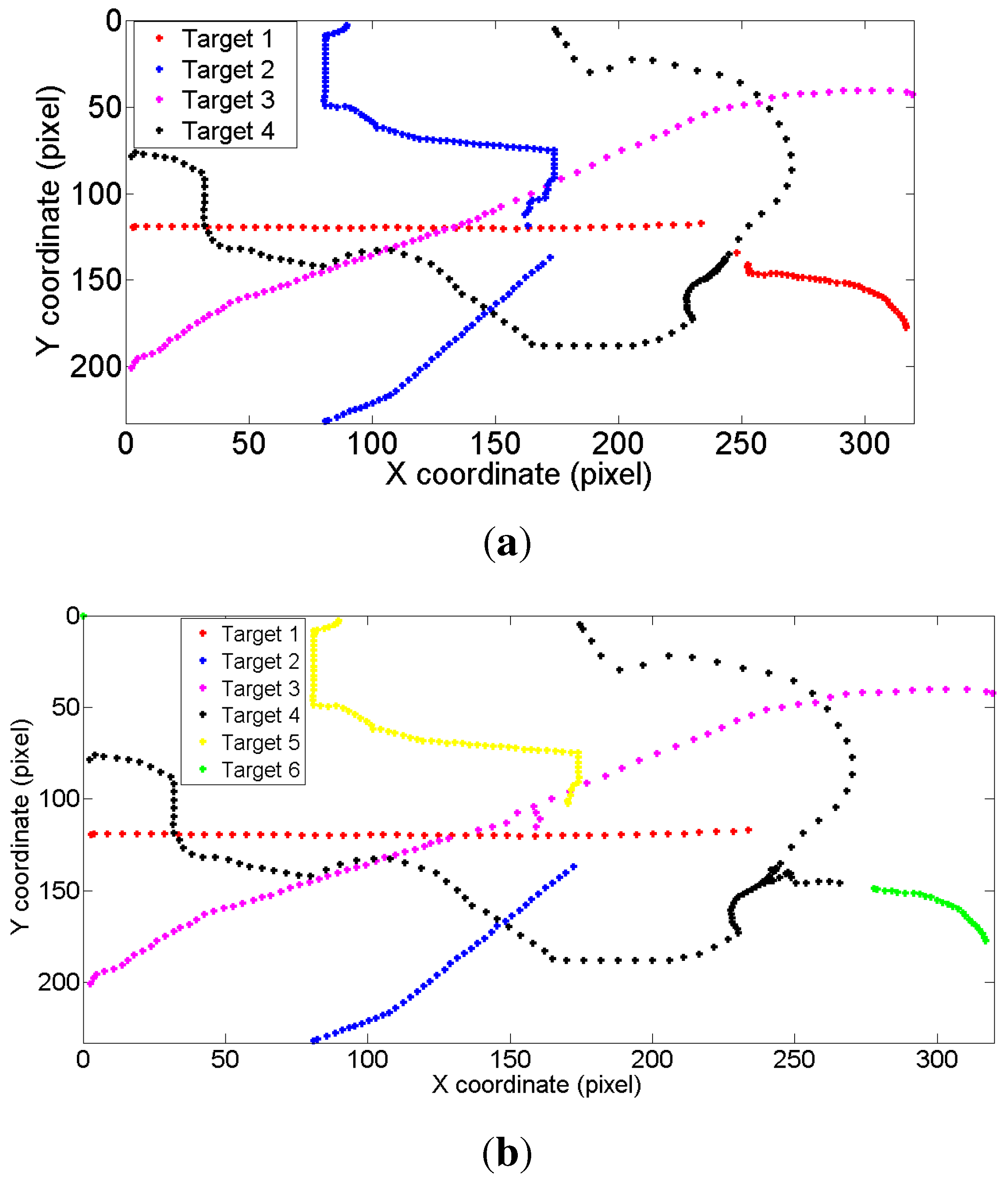
4.2. Evaluation of the Proposed Weight Penalization Method


| Tracker | Performance | Synthetic Images | Outdoor Human Surveillance | Cells Moving |
|---|---|---|---|---|
| GM-PHD | MOTA | 0.8586 | 0.6265 | 0.5128 |
| tracker [7] | MOTP | 0.9266 | 0.8567 | 0.4283 |
| CPGM-PHD | MOTA | 0.9863 | 0.7038 | 0.6842 |
| tracker [22] | MOTP | 0.9536 | 0.8724 | 0.5581 |
| Our | MOTA | 1 | 0.9348 | 0.7218 |
| tracker | MOTP | 0.9675 | 0.9273 | 0.6065 |
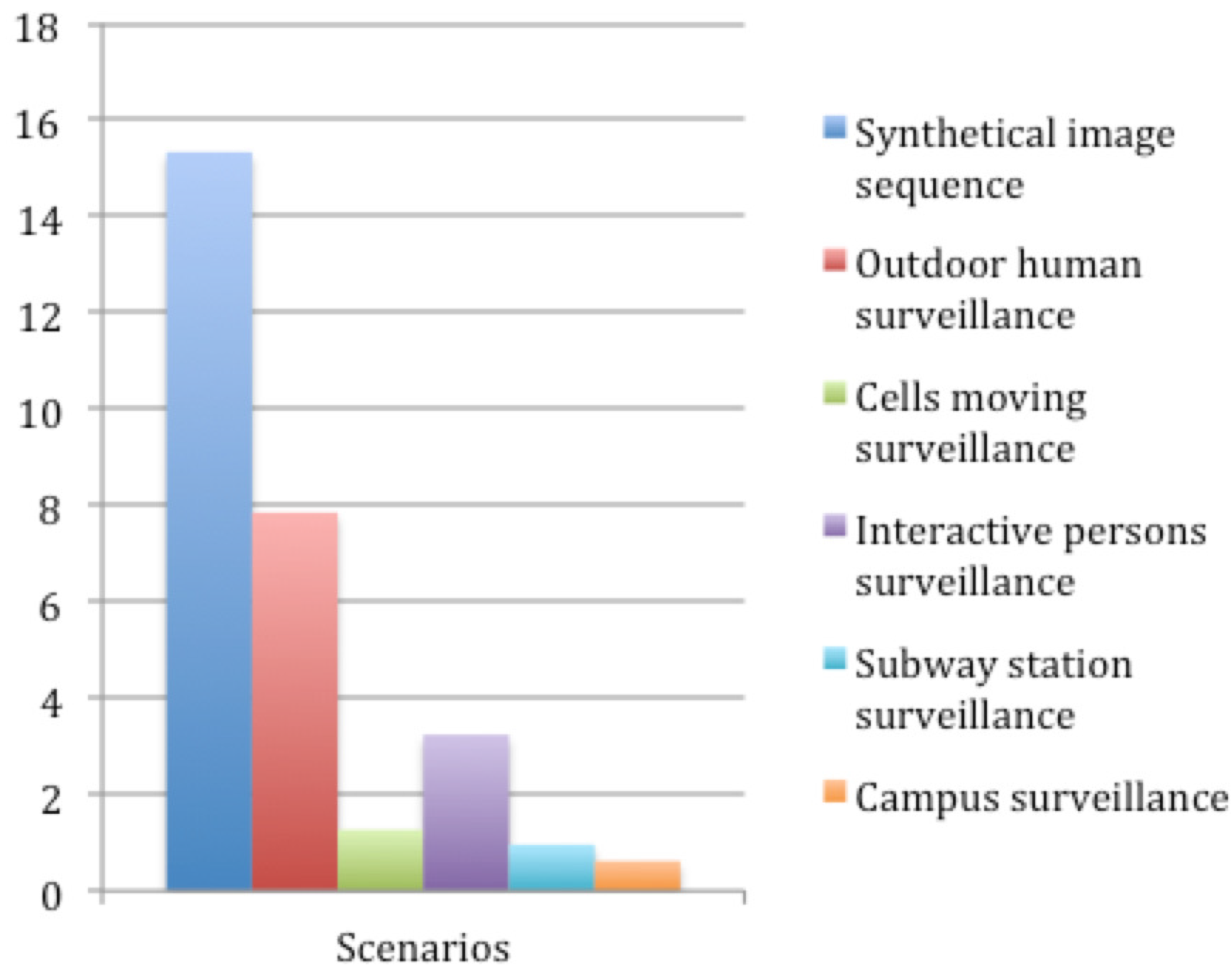
| Tracker | Synthetic Images | Outdoor Human Surveillance | Cells Moving |
|---|---|---|---|
| GM-PHD tracker | 12.88 | 8.52 | 18.75 |
| CPGM-PHD tracker | 1.37 | 2.76 | 7.13 |
| Our tracker | 0 | 0.94 | 2.68 |
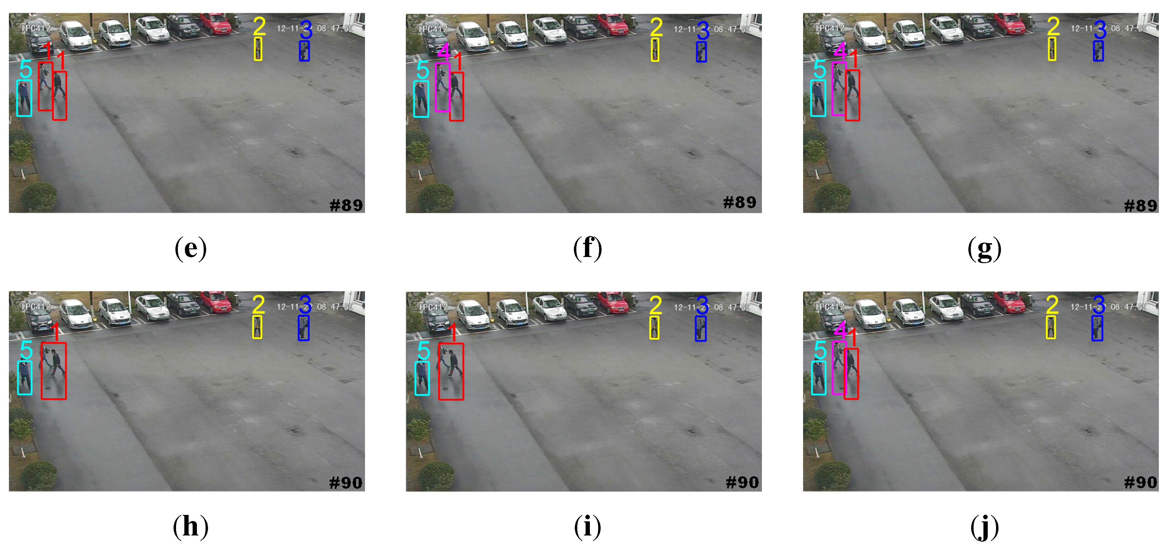
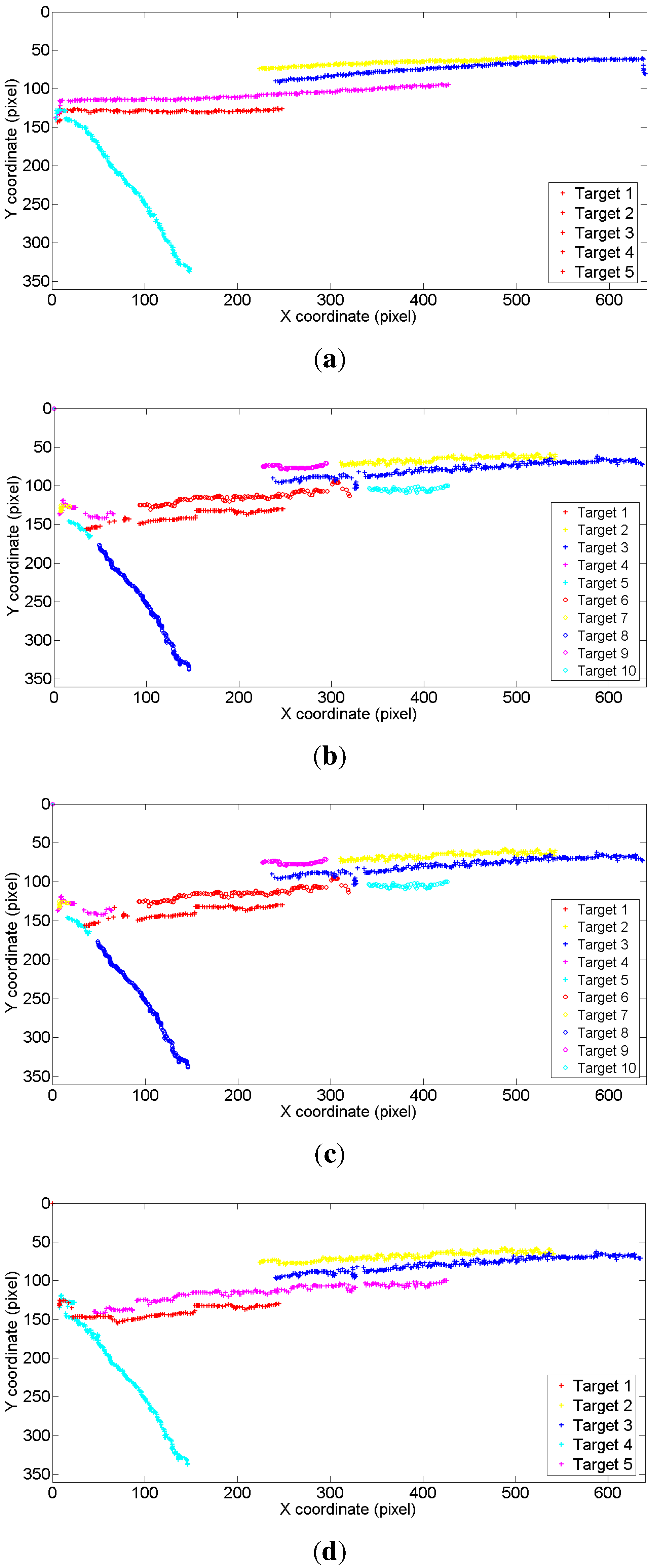
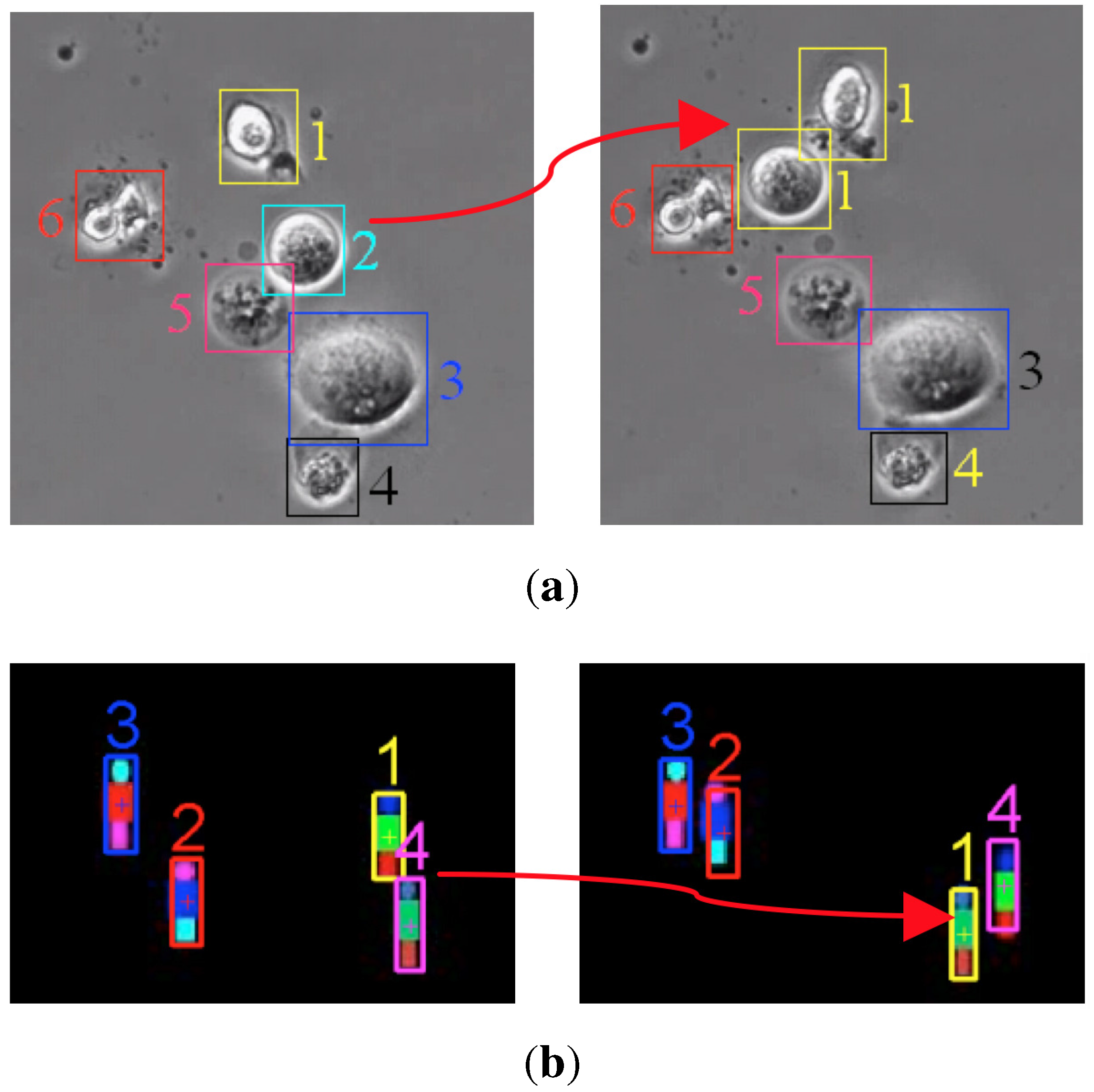
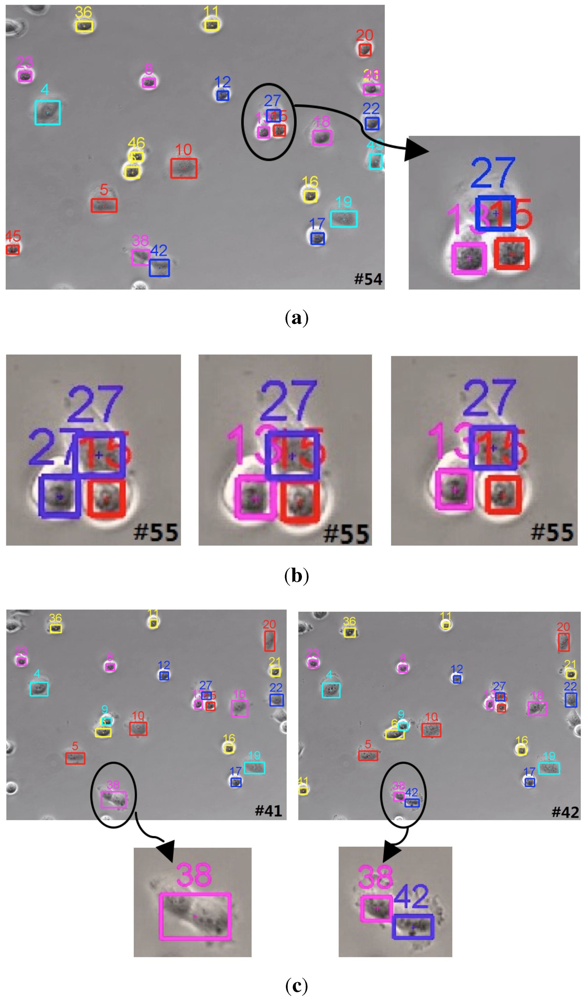
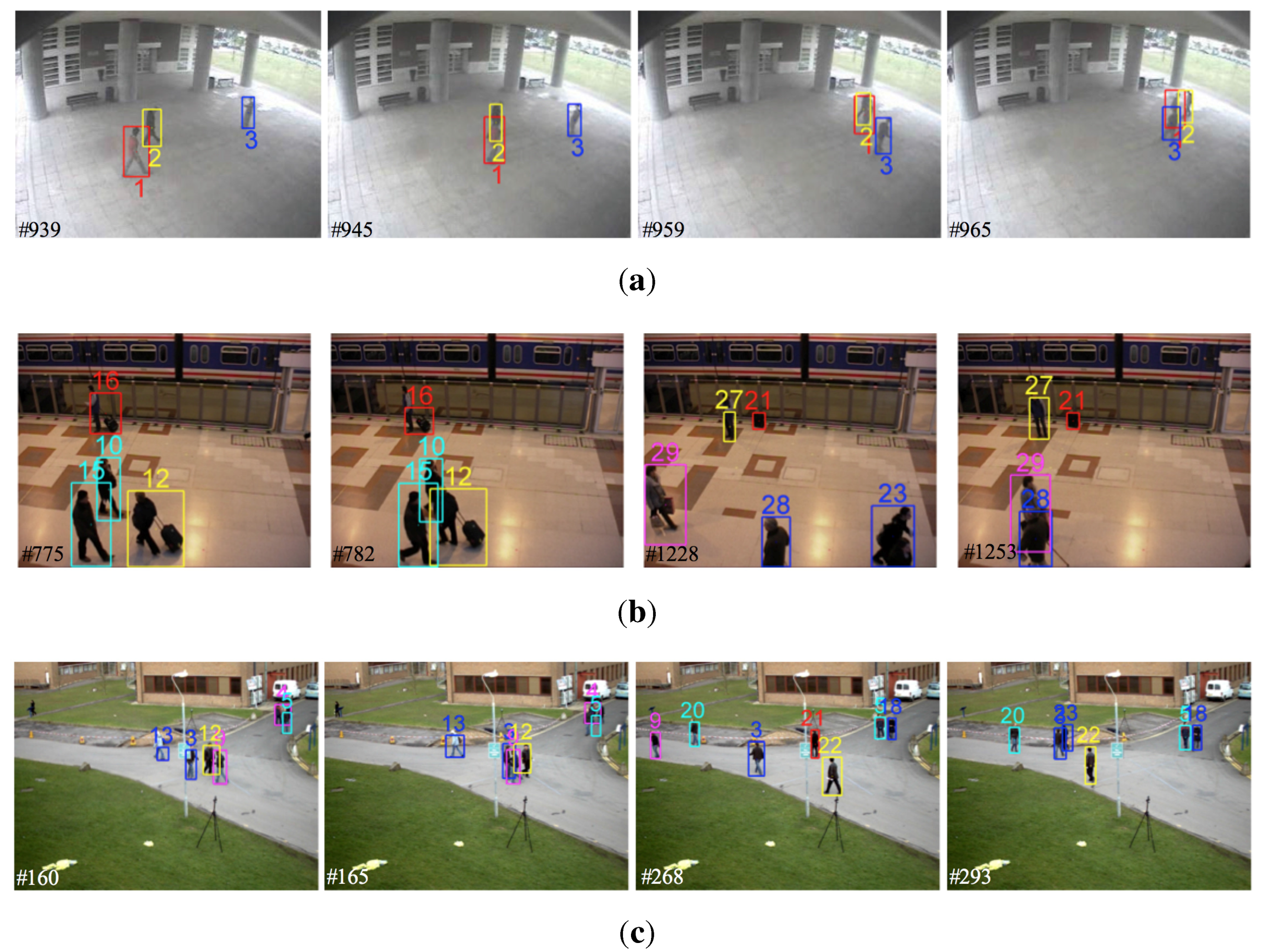
4.3. Evaluation of the Proposed Tracker
| GM-PHD Tracker [7] | Tracker in [31] | Tracker in [32] | Tracker in [33] | Our Tracker | |
|---|---|---|---|---|---|
| MOTA | 0.3440 | 0.9875 | 0.9221 | 0.9656 | 0.8861 |
| MOTP | 0.4286 | 0.5816 | 0.4980 | 0.5687 | 0.6346 |
| GM-PHD Tracker [7] | Tracker in [34] | Tracker in [35] | Tracker in [36] | Our Tracker | |
|---|---|---|---|---|---|
| MOTA | 0.4617 | 0.7591 | 0.8932 | 0.7977 | 0.8826 |
| MOTP | 0.4976 | 0.5382 | 0.5643 | 0.5634 | 0.6055 |

5. Conclusions
Acknowledgments
Author Contributions
Conflicts of Interest
References
- Zhou, S.; Fei, F.; Zhang, G.; Liu, Y.; Li, W.J. Hand-Writing Motion Tracking with Vision-Inertial Sensor Fusion: Calibration and Error Correction. Sensors 2014, 14, 15641–15657. [Google Scholar] [CrossRef] [PubMed]
- Choi, Y.J.; Kim, Y.G. A Target Model Construction Algorithm for Robust Real-Time Mean-Shift Tracking. Sensors 2014, 14, 20736–20752. [Google Scholar] [CrossRef] [PubMed]
- Bai, T.; Li, Y.; Zhou, X. Learning local appearances with sparse representation for robust and fast visual tracking. IEEE Trans. Cybern. 2015, 45, 663–675. [Google Scholar] [PubMed]
- Kwon, J.; Lee, K.M. Tracking by sampling and integrating multiple trackers. IEEE Trans. Pattern Anal. Mach. Intell. 2014, 36, 1428–1441. [Google Scholar]
- Park, C.; Woehl, T.; Evans, J.; Browning, N. Minimum cost multi-way data association for optimizing multitarget tracking of interacting objects. IEEE Trans. Pattern Anal. Mach. Intell. 2015, 37, 611–624. [Google Scholar] [CrossRef] [PubMed]
- Mahler, R. Multitarget bayes filtering via first-order multitarget moments. IEEE Trans. Aerosp. Electron. Syst. 2003, 39, 1152–1178. [Google Scholar] [CrossRef]
- Vo, B.N.; Ma, W. The Gaussian mixture probability hypothesis density filter. IEEE Trans. Signal Process. 2006, 54, 4091–4104. [Google Scholar] [CrossRef]
- Yoon, J.H.; Kim, D.Y.; Bae, S.H.; Shin, V. Joint initialization and tracking of multiple moving objects using doppler information. IEEE Trans. Signal Process. 2011, 59, 3447–3452. [Google Scholar] [CrossRef]
- Panta, K.; Clark, D.E.; Vo, B.N. Data association and track management for the Gaussian mixture probability hypothesis density filter. IEEE Trans. Aerosp. Electron. Syst. 2009, 45, 1003–1016. [Google Scholar] [CrossRef]
- Panta, K.; Clark, D.E.; Vo, B.N. Extended target tracking using a Gaussian-mixture PHD filter. IEEE Trans. Aerosp. Electron. Syst. 2012, 48, 3268–3286. [Google Scholar]
- Pham, N.T.; Huang, W.; Ong, S.H. Tracking multiple objects using probability hypothesis density filter and color measurements. In Proceedings of the 2007 IEEE International Conference on Multimedia and Expo, Beijing, China, 2–5 July 2007; pp. 1511–1514.
- Pham, N.T.; Huang, W.; Ong, S.H. Probability hypothesis density approach for multi-camera multi-object tracking. In Proceedings of the 8th Asian Conference on Computer Vision, Tokyo, Japan, 18–22 November 2007; pp. 875–884.
- Wu, J.; Hu, S. Probability hypothesis density filter based multi-target visual tracking. In Proceedings of the 2010 29th Chinese Control Conference (CCC), Beijing, China, 29–31 July 2010; pp. 2905–2909.
- Wu, J.; Hu, S.; Wang, Y. Probability-hypothesis-density filter for multitarget visual tracking with trajectory recognition. Opt. Eng. 2010, 49, 97011–97019. [Google Scholar] [CrossRef]
- Zhou, X.; Li, Y.; He, B. Entropy distribution and coverage rate-based birth intensity estimation in GM-PHD filter for multi-target visual tracking. Signal Process. 2014, 94, 650–660. [Google Scholar] [CrossRef]
- Zhou, X.; Li, Y.; He, B.; Bai, T. GM-PHD-based multi-target visual tracking using entropy distribution and game theory. IEEE Trans. Ind. Inform. 2014, 10, 1064–1076. [Google Scholar] [CrossRef]
- Pollard, E.; Plyer, A.; Pannetier, B.; Champagnat, F.; Besnerais, G.L. GM-PHD filters for multi-object tracking in uncalibrated aerial videos. In Proceedings of the 12th International Conference on Information Fusion (FUSION’09), Seattle, WA, USA, 6–9 July 2009; pp. 1171–1178.
- Clark, R.D.; Vo, B.N. Improved SMC implementation of the PHD filter. In Proceedings of the 2010 13th Conference on Information Fusion (FUSION), Edinburgh, UK, 26–29 July 2010; pp. 1–8.
- Maggio, I.E.; Taj, M.; Cavallaro, A. Efficient multi-target visual tracking using Random Finite Sets. IEEE Trans. Circuits Syst. Video Technol. 2008, 18, 1016–1027. [Google Scholar] [CrossRef]
- Yazdian-Dehkordi, M.; Azimifar, Z.; Masnadi-Shirazi, M. Competitive Gaussian mixture probability hypothesis density filter for multiple target tracking in the presence of ambiguity and occlusion. IET Radar Sonar Navig. 2012, 6, 251–262. [Google Scholar] [CrossRef]
- Yazdian-Dehkordi, M.; Azimifar, Z.; Masnadi-Shirazi, M. Penalized Gaussian mixture probability hypothesis density filter for multiple target tracking. Signal Process. 2012, 92, 1230–1242. [Google Scholar] [CrossRef]
- Wang, Y.; Meng, H.; Liu, Y.; Wang, X. Collaborative penalized Gaussian mixture PHD tracker for close target tracking. Signal Process. 2014, 102, 1–15. [Google Scholar] [CrossRef]
- Zhou, X.; Li, Y.; He, B. Game-theoretical occlusion handling for multi-target visual tracking. Pattern Recognit. 2013, 46, 2670–2684. [Google Scholar] [CrossRef]
- Wang, Y.; Wu, J.; Kassim, A.; Huang, W. Occlusion reasoning for tracking multiple people. IEEE Trans. Circuits Syst. Video Technol. 2009, 19, 114–121. [Google Scholar]
- Zhou, X.; Li, Y.; He, B. Multi-target visual tracking with game theory-based mutual occlusion handling. In Proceedings of the 2013 IEEE/RSJ International Conference on Intelligent Robots and Systems (IROS), Tokyo, Japan, 3–7 November 2013; pp. 4201–4206.
- Zhang, X.; Hu, W.; Luo, G.; Manbank, S. Kernel-bayesian framework for object tracking. In Proceedings of the 8th Asian Conference on Computer Vision, Tokyo, Japan, 18–22 November 2007; pp. 821–831.
- Wu, J.; Hu, S.; Wang, Y. Adaptive multifeature visual tracking in a probability-hypothesis-density filtering framework. Signal Process. 2013, 93, 2915–2926. [Google Scholar] [CrossRef]
- Lowe, D.G. Distinctive image features from scale-invariant keypoints. Int. J. Comput. Vis. 2004, 60, 91–110. [Google Scholar] [CrossRef]
- PETS2006. Available online: http://www.cvg.reading.ac.uk/PETS2006/data.html (accessed on 1 December 2015).
- PETS2009. Available online: http://www.cvg.reading.ac.uk/PETS2009/a.html (accessed on 1 December 2015).
- Zulkifley, M.A.; Moran, B. Robust hierarchical multiple hypothesis tracker for multiple-object tracking. Expert Syst. Appl. 2012, 39, 12319–12331. [Google Scholar] [CrossRef]
- Joo, S.W.; Chellappa, R. A multiple-hypothesis approach for multiobject visual tracking. IEEE Trans. Image Process. 2007, 16, 2849–2854. [Google Scholar] [CrossRef] [PubMed]
- Torabi, A.; Bilodeau, G.A. A multiple hypothesis tracking method with fragmentation handling. In Proceedings of the 2009 Canadian Conference on Computer and Robot Vision (CRV’09), Kelowna, BC, Canada, 25–27 May 2009; pp. 8–15.
- Yang, J.; Shi, Z.; Vela, P.; Teizer, J. Probabilistic multiple people tracking through complex situations. In Proceedings of the 9th International Symposium on Privacy Enhancing Technologies (PETS’09), Seattle, WA, USA, 5–7 August 2009; pp. 79–86.
- Andriyenko, A.; Schindler, K.; Roth, S. Discrete-continuous optimization for multi-target tracking. In Proceedings of the 2012 IEEE Conference on Computer Vision and Pattern Recognition (CVPR), Providence, RI, USA, 16–21 June 2012; pp. 1926–1933.
- Park, C.; Woehl, T.; Evans, J.; Browning, N. Online multiperson tracking-by-detection from a single, uncalibrated camera. IEEE Trans. Pattern Anal. Mach. Intell. 2011, 33, 1820–1833. [Google Scholar]
© 2015 by the authors; licensee MDPI, Basel, Switzerland. This article is an open access article distributed under the terms and conditions of the Creative Commons by Attribution (CC-BY) license (http://creativecommons.org/licenses/by/4.0/).
Share and Cite
Zhou, X.; Yu, H.; Liu, H.; Li, Y. Tracking Multiple Video Targets with an Improved GM-PHD Tracker. Sensors 2015, 15, 30240-30260. https://doi.org/10.3390/s151229794
Zhou X, Yu H, Liu H, Li Y. Tracking Multiple Video Targets with an Improved GM-PHD Tracker. Sensors. 2015; 15(12):30240-30260. https://doi.org/10.3390/s151229794
Chicago/Turabian StyleZhou, Xiaolong, Hui Yu, Honghai Liu, and Youfu Li. 2015. "Tracking Multiple Video Targets with an Improved GM-PHD Tracker" Sensors 15, no. 12: 30240-30260. https://doi.org/10.3390/s151229794
APA StyleZhou, X., Yu, H., Liu, H., & Li, Y. (2015). Tracking Multiple Video Targets with an Improved GM-PHD Tracker. Sensors, 15(12), 30240-30260. https://doi.org/10.3390/s151229794