Target Tracking and Classification from Labeled and Unlabeled Data in Wireless Sensor Networks

Abstract
: Tracking the locations and identities of moving targets in the surveillance area of wireless sensor networks is studied. In order to not rely on high-cost sensors that have been used in previous researches, we propose the integrated localization and classification based on semi-supervised learning, which uses both labeled and unlabeled data obtained from low-cost distributed sensor network. In our setting, labeled data are obtained by seismic and PIR sensors that contain information about the types of the targets. Unlabeled data are generated from the RF signal strength by applying Gaussian process, which represents the probability of predicted target locations. Finally, by using classified unlabeled data produced by semi-supervised learning, identities and locations of multiple targets are estimated. In addition, we consider a case when the labeled data are absent, which can happen due to fault or lack of the deployed sensor nodes and communication failure. We overcome this situation by defining artificial labeled data utilizing characteristics of support vector machine, which provides information on the importance of each training data point. Experimental results demonstrate the accuracy of the proposed tracking algorithm and its robustness to the absence of the labeled data thanks to the artificial labeled data.1. Introduction
Wireless sensor networks (WSNs) consist of small, low-power sensor nodes that collect, process, and communicate the sensor data. WSNs are suitable to monitor environmental phenomena widely distributed in space and time. This paper focuses on the problem of localization and classification of multiple targets moving within the area of deployed sensor nodes, which plays an important role in surveillance application [1], environmental monitoring [2–4], and traffic monitoring [5].
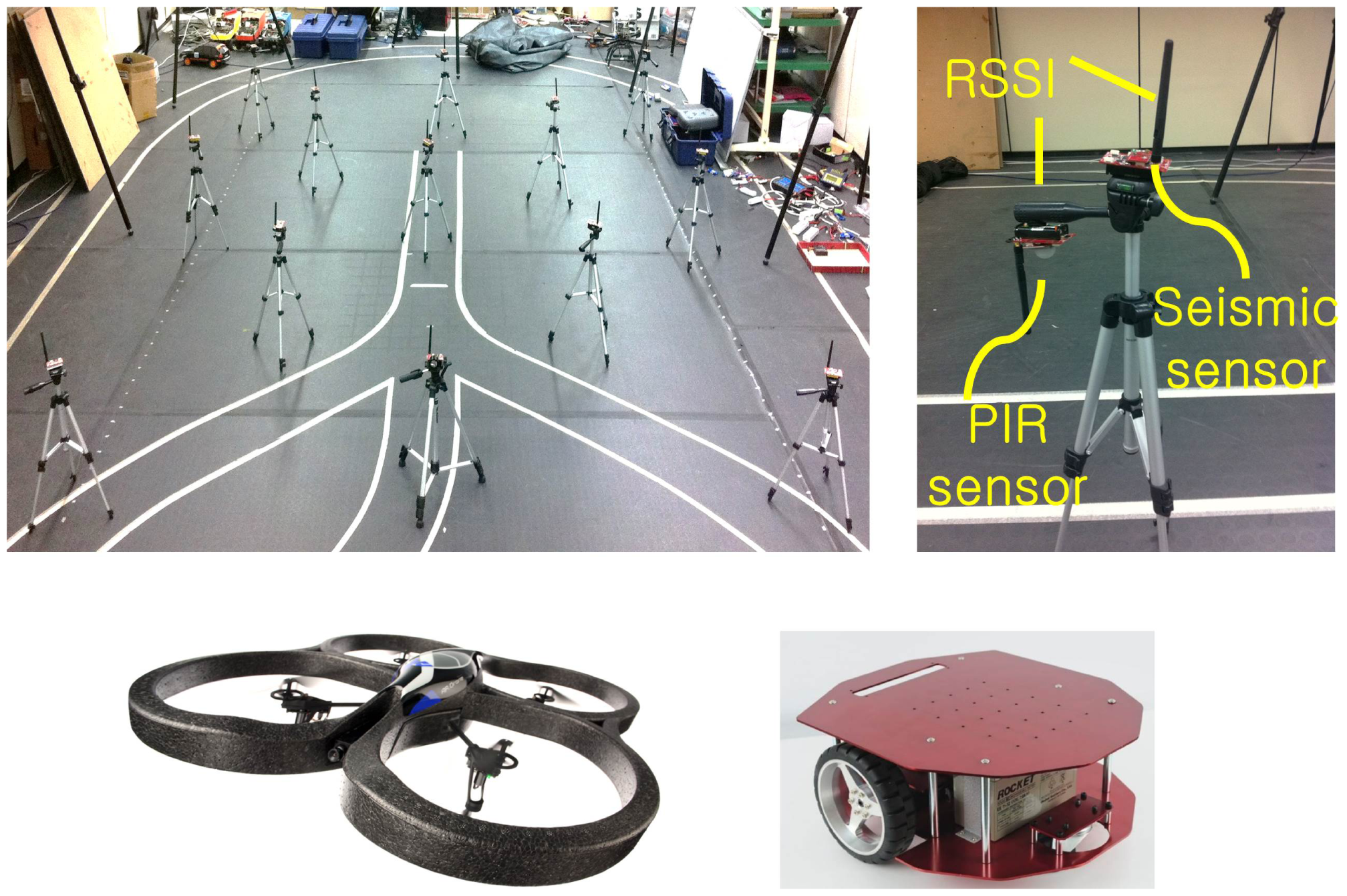
In particular, this paper considers low-cost sensors such as acoustic, magnetic, seismic, ultrasonic sensors and radio signal strength as shown in Figure 1, which consume low power. The low-cost sensors limit the direct adaptation of existing multi-target tracking algorithm due to following reasons. First, many multi-target tracking algorithms, such as Gaussian mixture probability hypothesis density filter [6], Markov chain Monte Carlo data association [7,8], assume that sensors measure location or both range and angle of targets, for example by using RFID [9], sonar, and LiDAR [10]. Generally, low-cost sensors such as RSSI measure relative distance to the target, not location. Therefore, without employing some additional data-association algorithms, it is difficult to directly adopt those algorithms [6–10] in our setup. Second, popular conventional localization algorithms such as time of arrival (TOA), time difference of arrival (TDOA) and angle of arrival (AOA) need expensive hardware [11,12] (e.g., laser) that is not available for the low-cost sensor nodes. Third, the memory and computational power in the low-cost sensor network are limited. There are existing classification methods such as fast Fourier transform (FFT) [13,14] and feature-aided tracking [15–17] in order to extract feature points from raw data. These need heavy computational load and large memory, which are intractable for low-cost sensor nodes without additional digital signal co-processors.
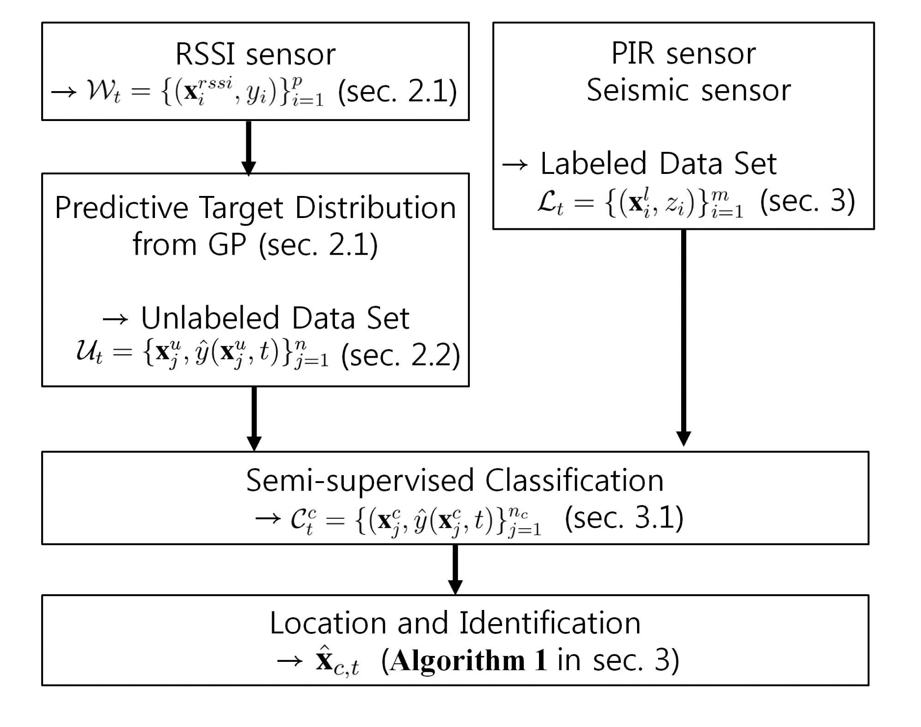
In order to meet the requirement of the multi-target tracking using low-cost sensor networks, we propose a new tracking algorithm based on semi-supervised learning as described in Figure 2. When a few labeled data are available, the semi-supervised learning [18] can efficiently utilize large amount of unlabeled data. In our experimental scenario, labeled data are obtained by deployed passive infrared (PIR) sensors and seismic sensors. This setup is suitable for semi-supervised learning because labeled data are sparsely obtained over space from those sensors due to their narrow sensing range relative to the wide surveillance area.
While labeled data present type information of heterogeneous targets, unlabeled data contain information about locations of targets. In the proposed framework, unlabeled data are generated from predictive target distribution that represents the probability of predicted target locations. To obtain the distribution from RSSI measurements, we employ Gaussian process (GP), which is a non-parametric machine learning technique. Due to its flexibility in modeling complex expressions using a small number of parameters, GP has been widely used to approximate signal strength [19].
Unlabeled data generated by GP contain information of target locations. Then, unlabeled data are classified via semi-supervised learning along with the small amount of labeled data, which provide information of both locations and identifications of targets. In other words, we can track targets using GP and semi-supervised learning in sequence.
We also propose a technique to deal with absence of labeled data, which can occur due to sensors fault, lack of the deployed sensors, or communication failure. We overcome this problem by propagating support vectors of each time instant, i.e., essential data points during classification, to the next time step and denning those that match with the incoming unlabeled data as artificial labeled data. This allows to maintain target tracking regardless of the existence of the labeled data.
The proposed algorithm is applied to an experiment for the tracking of moving aerial and ground vehicles, as shown in Figure 1. From the experiments with an actual wireless sensor network in a 4 m × 4 m surveillance area, our algorithm achieves good localization results. Moreover, the suggested algorithm is robust to the absence of the labeled data thanks to the artificial labeled data.
The rest of this paper is organized as follows. Section 2 introduces RSSI-based predictive target distribution using a Gaussian process. In Section 3, the tracking algorithm using semi-supervised learning is described. Section 4 shows the experimental results of tracking aerial and ground targets. Finally, Section 5 is devoted to concluding remarks.
2. RSSI-Based Predictive Target Distribution
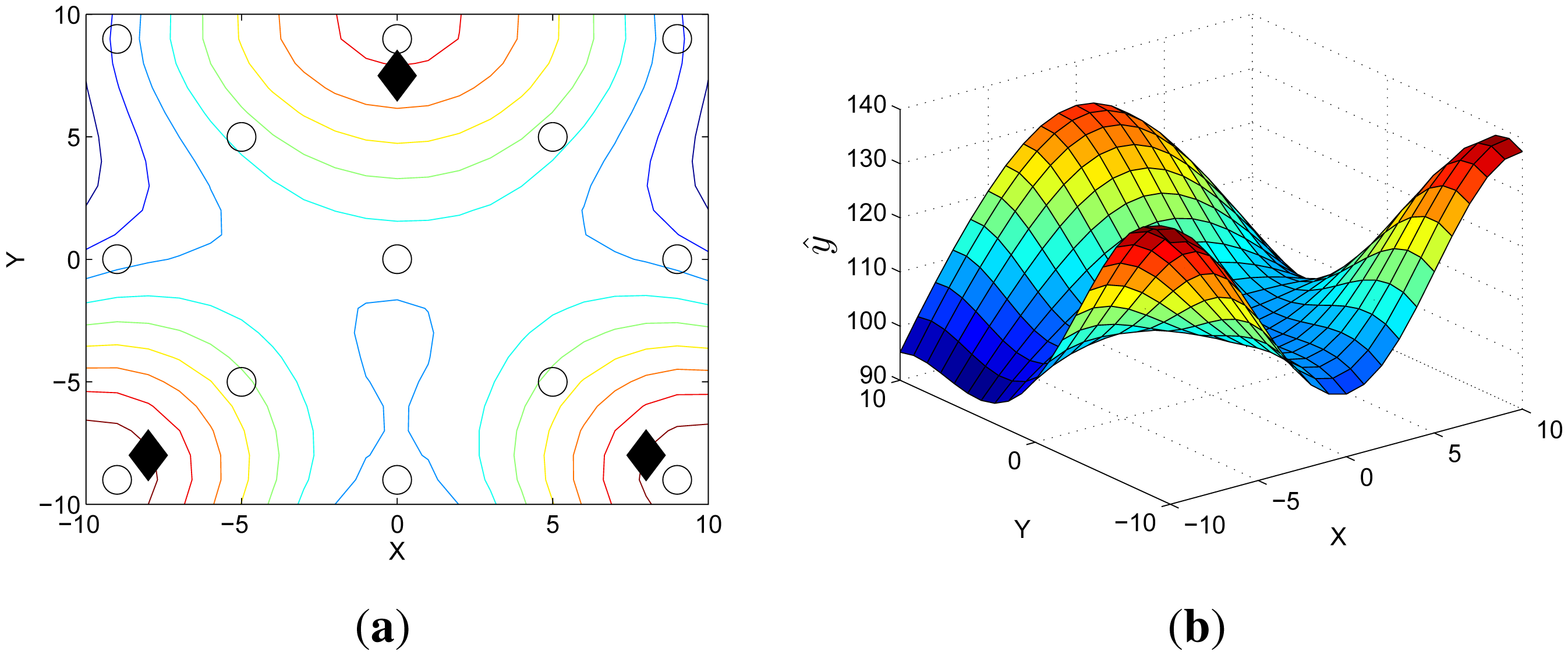
In received signal strength indication (RSSI)-based localization, the signal strength emitted by targets is measured by many sensors spatially distributed near the targets [20]. With the known locations of sensors, these measurements are used to make predictive target distribution that represents the probability of the predicted target locations. Figure 3 is a distribution example where 13 sensor nodes measure the RSSIs emitted from three targets.
Section 2.1 describes how the predictive target distribution is obtained by using a Gaussian process (GP). Section 2.2 shows how unlabeled data are generated from the constructed predictive target distribution.
2.1. Gaussian Process
Gaussian process for regression (GP) is a non-parametric regression model that defines a Gaussian distribution over output value for input value, conditioned on training data. The advantage of GP is its flexibility in modeling complex expressions under noise using a small number of learning parameters.
Let y1,…,yp be the measurement set where yi is the RSSI measurement obtained from the target nearest to the ith node and p is the number of RSSI sensor nodes. Also, sensor locations are defined as ,…, . Then, is the training set obtained from
 = {y1,…,yp}T is a function of the training inputs
, with the form
= {y1,…,yp}T is a function of the training inputs
, with the form
 ), (
) is p × p kernel matrix whose (i, j)th element is k(xi,xj). The squared exponential is a commonly used kernel function, given by
), (
) is p × p kernel matrix whose (i, j)th element is k(xi,xj). The squared exponential is a commonly used kernel function, given by
After the training, the GP estimates the output value of the Gaussian process for the input value that is an interested location x* = [X, Y]T ∈ χ, where χ is a user-defined set of the interested location and its cardinality is υ = |χ|. The output value has the mean ŷ(x*) and variance σ̂2(x*):
We note that ŷ(x*,t) represents the GP estimation at time step t.
Example 1
Figure 3b is an example of the distribution obtained by the GP where χ is defined as {(X, Y) : X, Y ∈ {−10,…,10}} and the values on the z-axis are the estimated means. When using the RSSI measurements as the input of the GP and the corresponding locations as the output of the GP, the distribution represents the predicted sensor measurements over the space as illustrated in Figure 3b. More specifically, the estimated ŷ(x*) indicates the predicted RSSI measurement of an artificial sensor that does not exist at x*. Because the RSSI value is larger when the target is closer, the value on the z-axis of the distribution, ŷ, implies the probability with which the targets are located at (X, Y).
2.2. Unlabeled Data Generation
We highlight again that larger value on the z-axis of the predictive target distribution denotes higher probability of the predicted locations of targets. In this manner, we derive a dataset
for xu ∈ x from the predictive target distribution satisfying
where yth is a user-defined threshold. Thus, the dataset
 t are correlated with the predictive locations of the targets at time t. Depending on the value of yth, the amount of unlabeled data is decided. As described in Figure 3b, the value larger than 130 can be considered high probability for the target locations. For this reason, we set yth = 130 in this paper.
We assume that sensor nodes do not know the labels of the RSSI measurements, i.e., the nodes do not know who emitted the RF signal. With this assumption, the dataset
t does not provide any information about identity of the targets. In the following section, we introduce a semi-supervised algorithm to classify the unlabeled data in order to identify the targets.
3. Target Tracking Based on Semi-Supervised Learning
Traditional classification algorithms such as supervised learning are inaccurate when only a few labeled data are available. To overcome this problem, semi-supervised classification [21,22] improves the efficiency and performance of supervised learning by using both labeled and unlabeled data.
We assume that N different targets are identified by the identification label set {1,…, N}. There is a small set of labeled data, given by , where is the location of the ith labeled data and is the observation denoting the identification label of the targets.
We describe the Laplacian support vector machine (LapSVM) algorithm in Section 3.1. The best scenario for semi-supervised classification is where there always exists at least one labeled data for each class while tracking the target. However, this cannot be guaranteed due to sensor fault, lack of deployed sensor, or communication failure. Considering a case where there is no labeled data at some time instants, we propose incremental learning for target tracking in Section 3.2.
3.1. Laplacian Support Vector Machine (LapSVM)
In the graph-based semi-supervised classification algorithm, the geometry of data is represented by an undirected graph
 = (V, E) with nodes V = {1,…, n + m} and edges E, where n and m are the number of unlabeled and labeled data, respectively. The nodes V represent the training data, and the edges E denote the similarities between the nodes. These similarities are given by the connection strength from a node i to another node j, which is encoded in the element Wij, of a weight matrix W. A typical weight matrix is given by the a Gaussian function of the Euclidean distance between data, with length scale θ3:
, the graph Laplacian matrix is defined as
The semi-supervised learning algorithm outputs an (n + m)-dimensional real-valued vector f* = [f(x1),f(x2),…,f(xn+m)]T, where . In the LapSVM algorithm, optimal α* = [α1,…,αn+m]T is given by
The optimal β* in order to get the optimal α* in Equation (7) is obtained by the following quadratic program:
In the semi-supervised learning, the unlabeled data help finding the decision boundary more accurately, assuming that data points of each class tend to form a cluster (called cluster assumption [21]). In other words, if points are in the same cluster, they are likely to belong to the same class.
Example 2
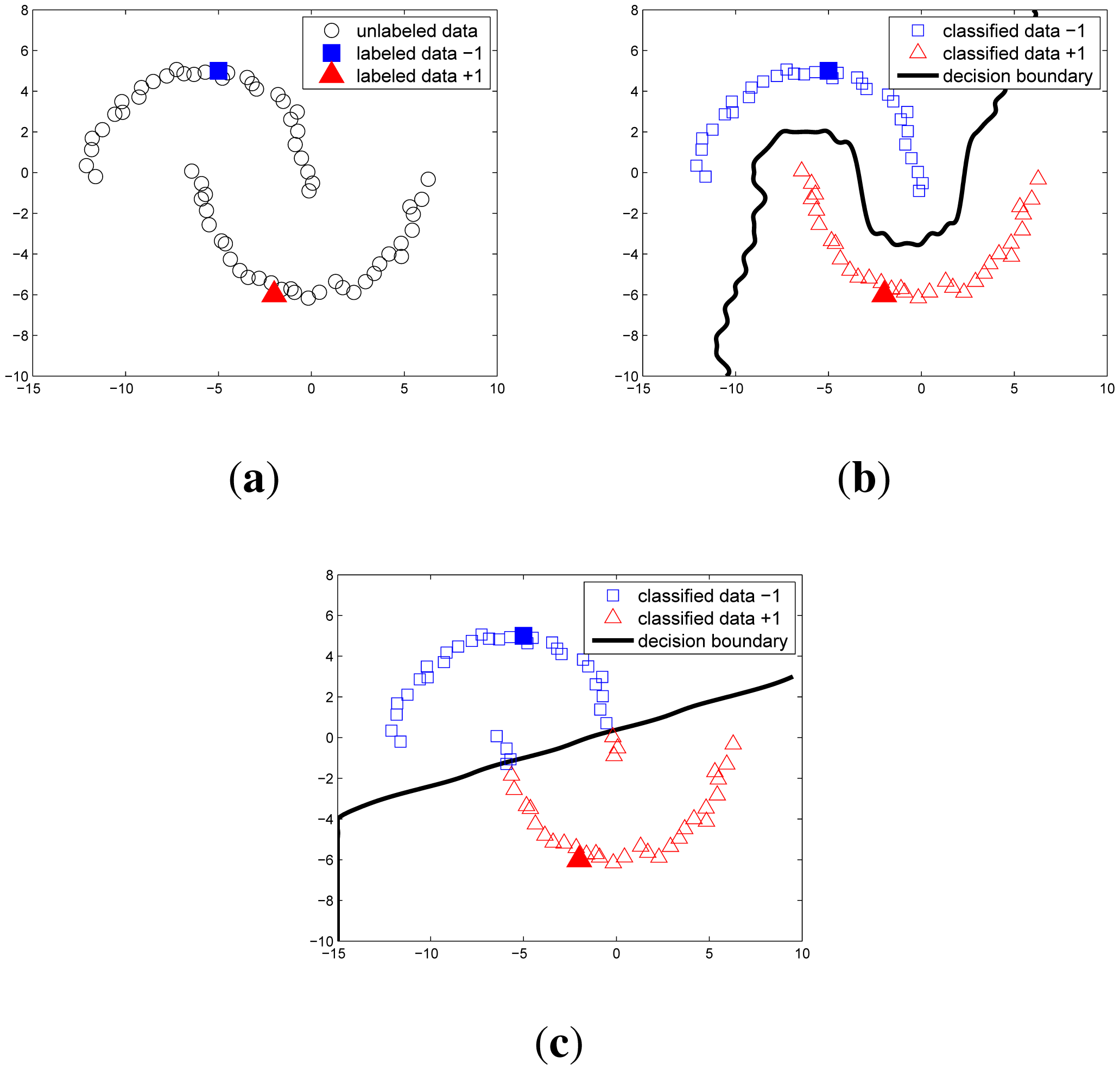
Figure 4 illustrates the two-moon classification problem. In order to show the usefulness of unlabeled data, we prepare only one labeled data for each class. In the semi-supervised algorithm, the adjacent points in a high-density data region are classified into the same class. This gives a correct decision boundary, in contrast to the supervised learning shown in Figure 4c. The influence of the unlabeled data in this algorithm is handled by γI in Equation (7). When γI = 0, Equation (7) gives zero coefficients over the unlabeled data, so the algorithm becomes standard supervised SVM. On the other hand, as γI increases, the effect of unlabeled data also increases. In this paper, we set γI = 103 and γA = 0.1.
General classification algorithm presets the label value to +1 or −1 and appoints the label of an unlabeled data xu based on the function f : if f(xu) > 0 then the label of xu is +1, or if f(xu) ≤ 0 then the label of xu is −1. For the multi-label classification problem, it can be solved using “One Against One” or “One Against All” algorithms [23]. Specific descriptions of these algorithms are out of the scope of this paper. Instead, we define Q(x) as a function mapping the data to the label. Therefore, all data points , 1 ≤ i ≤ n will have labels through the classifier, given by , where N is the number of identification labels. For example, we consider two types of targets to track, thus N = 2.
As the result of classification, we define
as classified sets to label c, given by
, where nc is the number of data points that are labeled to c. The total set and number of unlabeled data,
t and n described in Section 2.2, can be described by
and
.
3.2. Incremental Time Series Classification
We consider a situation where there is no labeled data after the targets intrude the surveillance field. Most papers assume that initial positions of the intruders are successfully estimated by deploying sensor nodes intensively at edge of the surveillance field. Accordingly, we also assume that the set of labeled data exists at the moment the targets just enter the surveillance area. In this section, we focus on how to perform semi-supervised classification when labeled data is absent after the target intruded.
Target information at the current time step is correlated with the information at the previous time step such as a Markov process model. This leads us to exploit the classified data at the previous time step to create artificial labeled data for the current time step (artificial labeled data is different with the genuine labeled data made by the sensor). Our strategy is to select useful data among the classified datasets at the previous time step and define them as the artificial labeled data for the current time step.
The support vector machine framework offers a natural method to select such useful data. The classification rule is based on the decision boundary that depends on the support vector, xi with |αi| < 0 in Equation (7), in the SVM algorithm. In other words, the support vectors are representative points of the classification result. Moreover, once the data is well trained, most of the α's become zero and only a few support vectors have nonzero value of the coefficient |α|. Therefore, the small set of support vectors is suitable to be propagated to the next step and they become candidates for artificial labeled data.
One more consideration in constructing the artificial labeled data is that they have to be updated as time elapses. Some candidates obtained during the previous time step may not correlate with the current data. In order to find correlated points among the candidates to the current data, we check whether the candidates belong to the current unlabeled dataset or not. The candidates satisfying this condition become the artificial labeled data at time t, given by where sc is the number of the artificial labeled data that are labeled to c.
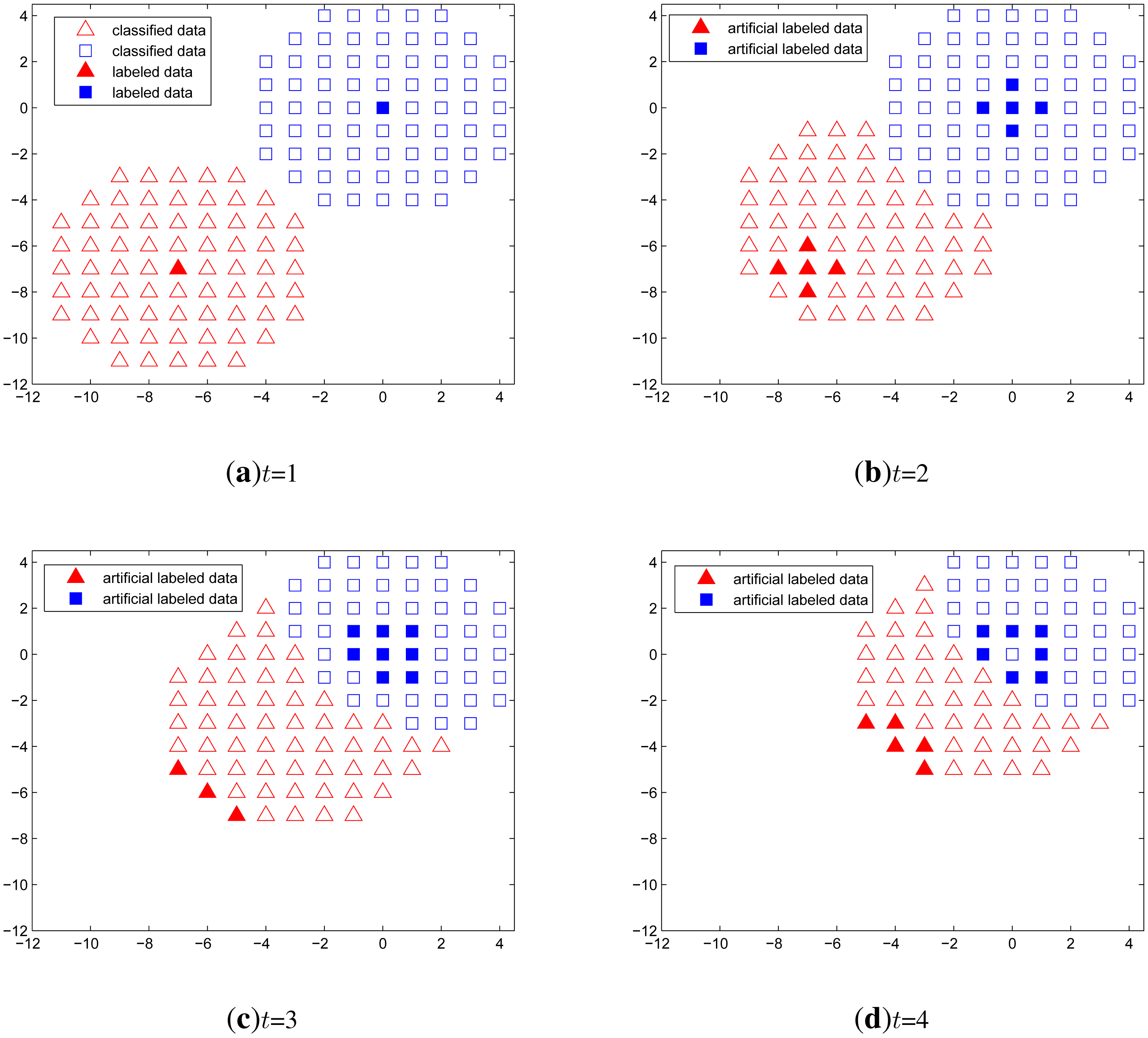
Example 3
Figure 5 shows a time series classification example when no labeled data exist except in the first time step. In this simulation, we let one target remain at the origin all the time and the other approaches the origin. The unlabeled data are generated over a circular region around the two targets. The expected incorrect outcome is that one classified set is merged into the other set, which wrongly represents multiple overlapping targets as one identity. However, from the simulation results, the classification using only the artificial labeled data performs well both when the targets are approaching and when the targets are apart from each other.
Concluding this section, we summarize a procedure for multi-target localization and classification into Algorithm 1.
| Algorithm 1 Multi-target localization and classification. |
| Step 1: Collect p RSSI measurement dataset |
| Step 2: Collect m labeled dataset |
| Step 3: Generate the predictive target distribution (Section 2.1) |
| Step 4: Obtain unlabeled dataset from the predictive target distribution . (Section 2.2) |
| Step 5: If t ≥ 2, generate artificial labeled data , then renew . (Section 3.2) |
| Step 6: Execute the LapSVM classification algorithm, then obtain the classified dataset . (Section 3.1) |
| Step 7: Estimate the positions of the targets x̂c,t for c = {1,…,N}: |
| , |
| , |
| where . |
| Step 8: t←t + 1, then go to Step1. |
4. Experiment
This section describes experimental setup, characteristics of sensor data, ( i.e., PIR, seismic, RSSI sensors), and tracking results.
4.1. Setup
We consider a two-dimensional tracking problem for one ground and one aerial target using a total of 26 sensor nodes. To identify the aerial vehicle, 13 spatially distributed seismic sensors are used to recognize the airflow due to aerial vehicle. The ground vehicle is identified by 13 passive infrared sensors (PIR). In addition, RSSI is available for both types of sensor nodes. The true trajectories of the targets are obtained by a Vicon Motion System that tracks reflective markers attached to each target.
4.2. Characteristics of Sensor Data
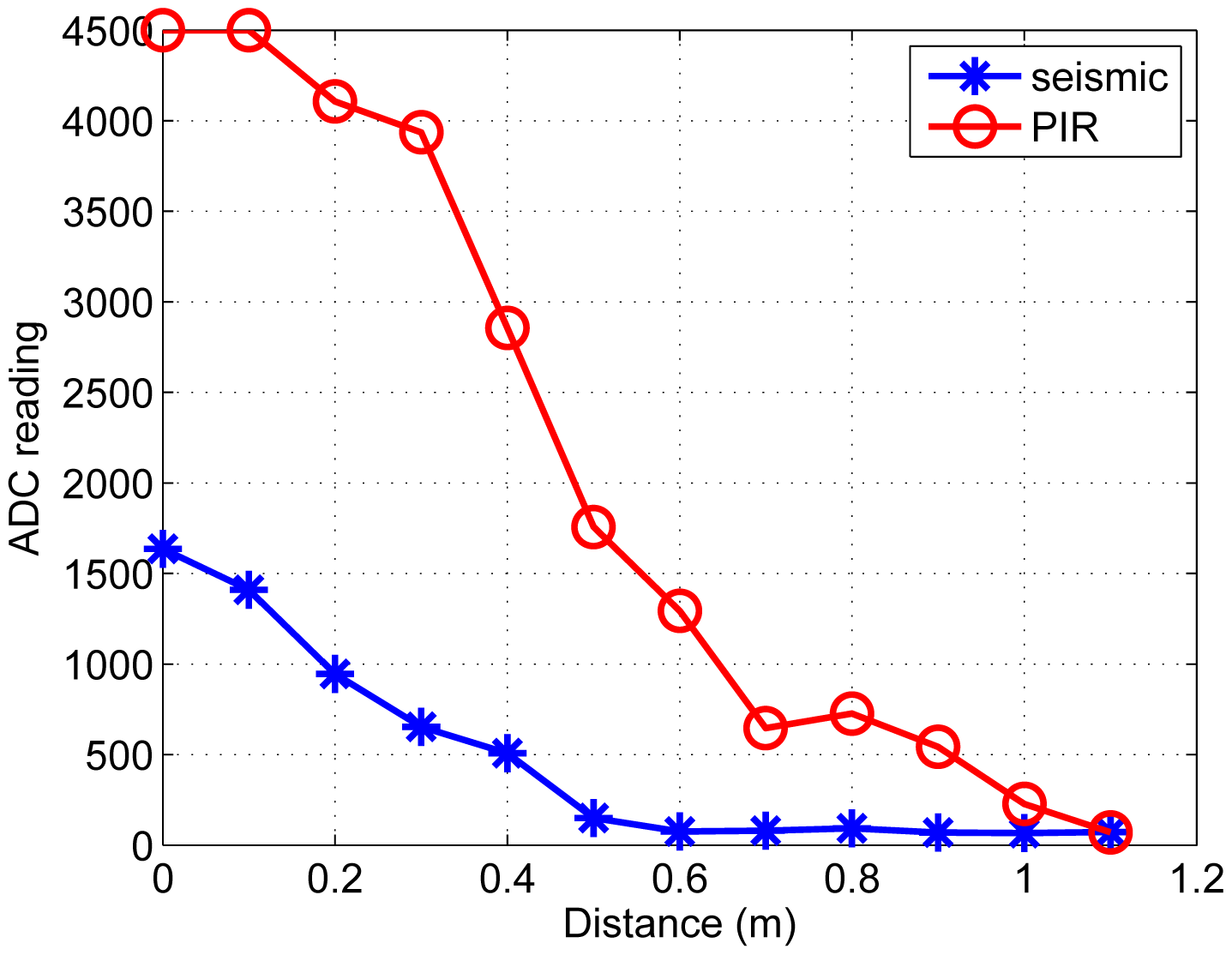
We record the raw ADC readings of one PIR sensor by varying the distance between the node and the ground target. Similarly, the raw ADC of one seismic sensor is measured using the aerial target, shown in Figure 6. We set threshold values to each sensor, i.e., 300 for the seismic sensor and 500 for the PIR sensor. Based on the defined thresholds on readings, the ith seismic sensor node yields +1 labeled data when a reading is greater than the threshold, i.e., zi = +1. Similarly, the jth PIR sensor node generates −1 labeled data, i.e., zj = −1.
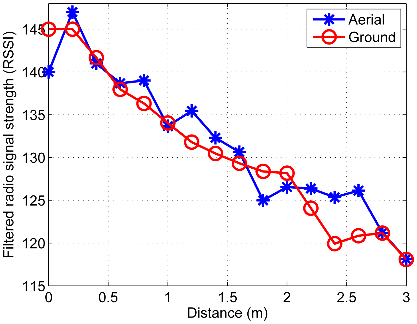
Besides, all 26 sensor nodes measure the RSSI. Considering the noisy ADC reading of the RSSI, moving average filter [24] is adopted. Figure 7 shows the relationship between the filtered RSSI measurement and the distance between a node and the ground target and the aerial target, respectively.
4.3. Tracking Results
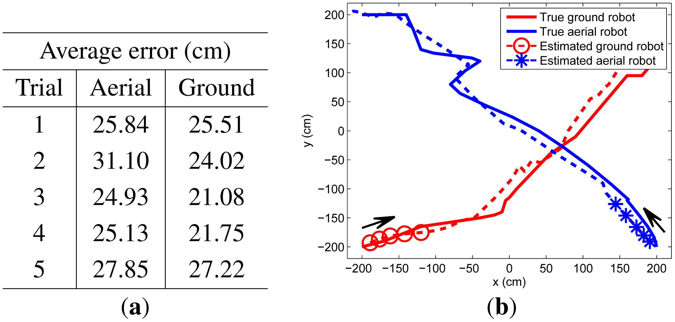
In our experiments, two targets start from different corners of the surveillance area, crossing at the middle of their pathway. We perform five trials, whose results are summarized in Figure 8. Because the RSSI characteristics are affected by the motion of the flying aerial robot, its tracking results are worse than results of the ground robot.
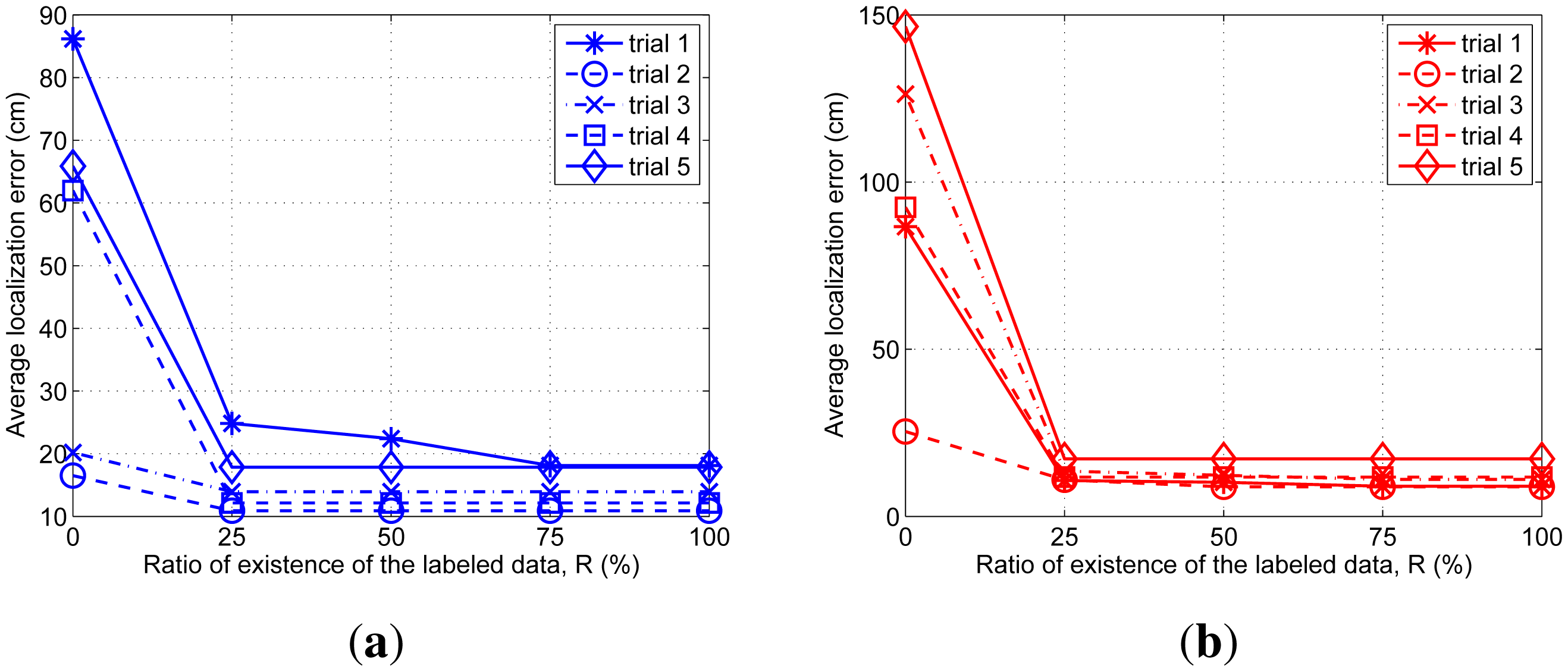
Moreover, we analyze the effect of the artificial labeled data introduced in Section 3.2 with respect to the ratio of existence of the labeled data, R:
We intentionally remove the labeled data among the data obtained via the experiment up to each 25%, 50%, 75% 100%, and then perform tracking. The results of the average localization error for each aerial and ground targets are summarized in Figure 9.
When there is no labeled data all the time (R = 0%), four of the five results do not indicate the correct trajectories. From 25% to 100% of the existence ratio of the labeled data, the results are almost same as the results for 100% absence ratio. We confirm that the artificial labeled data prevent the tracking performance from getting deteriorated by the lack of the labeled data.
5. Conclusions
This paper proposed a new multi-target localization and classification for low-cost sensor networks. Data configuration that consists of the unlabeled and labeled data obtained from low-cost sensor nodes was well-suited to apply semi-supervised learning. Furthermore, the incremental algorithm was developed with semi-supervised learning to handle the situation where labeled data are absent. The suggested algorithm was evaluated for the tracking of aerial and ground targets and showed accurate tracking performance and robustness to the absence of labeled data.
Acknowledgments
This work was supported by the National Research Foundation of Korea (NRF) grant funded by the Ministry of Science, ICT & Future Planning (MSIP), and the Korea government (MEST).
Author Contributions
Jaehyun Yoo and Hyoun Jin Kim designed the tracking algorithm; Jaehyun Yoo performed the experiments and analyzed the data; Jaehyun Yoo and Hyoun Jin Kim wrote the paper
Conflicts of Interest
The authors declare no conflict of interest
References
- Chen, M.; González, S.; Cao, H.; Zhang, Y.; Vuong, S.T. Enabling low bit-rate and reliable video surveillance over practical wireless sensor network. J. Supercomput. 2013, 65, 287–300. [Google Scholar]
- Song, G.; Zhou, Y.; Ding, E.; Song, A. A mobile sensor network system for monitoring of unfriendly environments. Sensors 2008, 8, 7259–7274. [Google Scholar]
- Wan, J.; Yu, Y.; Wu, Y.; Feng, R.; Yu, N. Hierarchical leak detection and localization method in natural gas pipeline monitoring sensor networks. Sensors 2012, 12, 189–214. [Google Scholar]
- Lloret, J.; Bosch, I.; Sendra, S.; Serrano, A. A wireless sensor network for vineyard monitoring that uses image processing. Sensors 2011, 11, 6165–6196. [Google Scholar]
- Torfs, T.; Sterken, T.; Brebels, S.; Santana, J.; van den Hoven, R.; Spiering, V.; Bertsch, N.; Trapani, D.; Zonta, D. Low power wireless sensor network for building monitoring. IEEE Sens. J. 2013, 13, 909–915. [Google Scholar]
- Vo, B.N.; Ma, W.K. The Gaussian mixture probability hypothesis density filter. IEEE Trans. Signal Process. 2006, 54, 4091–4104. [Google Scholar]
- Oh, S.; Russell, S.; Sastry, S. Markov chain Monte Carlo data association for multi-target tracking. IEEE Trans. Autom. Control 2009, 54, 481–497. [Google Scholar]
- Liu, J.; Chu, M.; Reich, J.E. Multitarget tracking in distributed sensor networks. IEEE Signal Process. Mag. 2007, 24, 36–46. [Google Scholar]
- Shin, J.; Lee, N.; Thrun, S.; Guibas, L. Lazy inference on object identities in wireless sensor networks. Proceedings of the 4th International Symposium on Information Processing in Sensor Networks, Los Angeles, CA, USA, 25–27 April 2005; p. 23.
- Nelson, J.K.; Roufarshbaf, H. A tree search approach to target tracking in clutter. Proceedings of the 12th International Conference on Information Fusion (FUSION'09), Seattle, WA, USA, 6–9 July 2009; pp. 834–841.
- Bachrach, J.; Taylor, C. Localization in sensor networks. In Handbook of Sensor Networks: Algorithms and Architectures; Wiley: Hoboken, NJ, USA, 2005; Volume 1. [Google Scholar]
- Vercauteren, T.; Guo, D.; Wang, X. Joint multiple target tracking and classification in collaborative sensor networks. IEEE J. Sel. Areas Commun. 2005, 23, 714–723. [Google Scholar]
- Bilik, I.; Tabrikian, J.; Cohen, A. GMM-based target classification for ground surveillance Doppler radar. IEEE Trans. Aerosp. Electron. Syst. 2006, 42, 267–278. [Google Scholar]
- Duarte, M.F.; Hu, Y.H. Vehicle classification in distributed sensor networks. J. Parallel Distrib. Comput. 2004, 64, 826–838. [Google Scholar]
- Roufarshbaf, H.; Nelson, J.K. Feature-aided initiation and tracking via tree search. Proceedings of the 2013 Asilomar Conference on Signals, Systems and Computers, Pacific Grove, CA, USA, 3–6 November 2013; pp. 2138–2142.
- Hong, L.; Cui, N.; Pronobis, M.; Scott, S. Local motion feature aided ground moving target tracking with GMTI and HRR measurements. IEEE Trans. Autom. Control 2005, 50, 127–133. [Google Scholar]
- Brown, A.P.; Sullivan, K.J.; Miller, D.J. Feature-Aided Multiple Target Tracking in the Image Plane. Proc. SPIE 2006. [Google Scholar] [CrossRef]
- Chapelle, O.; Schölkopf, B.; Zien, A. Semi-Supervised Learning; MIT Press: Cambridge, MA, USA, 2006; Volume 2. [Google Scholar]
- Yoo, J.H.; Kim, W.; Kim, H.J. Event-driven Gaussian process for object localization in wireless sensor networks. Proceedings of the 2011 IEEE/RSJ International Conference on Intelligent Robots and Systems (IROS), San Francisco, CA , USA, 25–30 September 2011; pp. 2790–2795.
- Sugano, M.; Kawazoe, T.; Ohta, Y.; Murata, M. Indoor localization system using RSSI measurement of wireless sensor network based on ZigBee standard. Target 2006, 538, 050. [Google Scholar]
- Belkin, M.; Niyogi, P.; Sindhwani, V. Manifold regularization: A geometric framework for learning from labeled and unlabeled examples. J. Mach. Learn. Res. 2006, 7, 2399–2434. [Google Scholar]
- Guillaumin, M.; Verbeek, J.; Schmid, C. Multimodal semi-supervised learning for image classification. Proceedings of the 2010 IEEE Conference on Computer Vision and Pattern Recognition (CVPR), San Francisco, CA, USA, 13–18 June 2010; pp. 902–909.
- Tsujinishi, D.; Koshiba, Y.; Abe, S. Why pairwise is better than one-against-all or all-at-once. Proceedings of the 2004 IEEE International Joint Conference on Neural Networks, Budapest, Hungary, 25–29 July 2004; 1.
- Smith, S.W. The Scientist and Engineer's Guide to Digital Signal Processing; California Technical Pub: San Diego, CA, USA, 1997. [Google Scholar]


© 2014 by the authors; licensee MDPI, Basel, Switzerland. This article is an open access article distributed under the terms and conditions of the Creative Commons Attribution license ( http://creativecommons.org/licenses/by/4.0/).
Share and Cite
Yoo, J.; Kim, H.J. Target Tracking and Classification from Labeled and Unlabeled Data in Wireless Sensor Networks. Sensors 2014, 14, 23871-23884. https://doi.org/10.3390/s141223871
Yoo J, Kim HJ. Target Tracking and Classification from Labeled and Unlabeled Data in Wireless Sensor Networks. Sensors. 2014; 14(12):23871-23884. https://doi.org/10.3390/s141223871
Chicago/Turabian StyleYoo, Jaehyun, and Hyoun Jin Kim. 2014. "Target Tracking and Classification from Labeled and Unlabeled Data in Wireless Sensor Networks" Sensors 14, no. 12: 23871-23884. https://doi.org/10.3390/s141223871
APA StyleYoo, J., & Kim, H. J. (2014). Target Tracking and Classification from Labeled and Unlabeled Data in Wireless Sensor Networks. Sensors, 14(12), 23871-23884. https://doi.org/10.3390/s141223871