The Influence of Random Element Displacement on DOA Estimates Obtained with (Khatri–Rao-)Root-MUSIC


Abstract
: Although a wide range of direction of arrival (DOA) estimation algorithms has been described for a diverse range of array configurations, no specific stochastic analysis framework has been established to assess the probability density function of the error on DOA estimates due to random errors in the array geometry. Therefore, we propose a stochastic collocation method that relies on a generalized polynomial chaos expansion to connect the statistical distribution of random position errors to the resulting distribution of the DOA estimates. We apply this technique to the conventional root-MUSIC and the Khatri-Rao-root-MUSIC methods. According to Monte-Carlo simulations, this novel approach yields a speedup by a factor of more than 100 in terms of CPU-time for a one-dimensional case and by a factor of 56 for a two-dimensional case.1. Introduction
DOA estimation is a major application of the sensor array, since there are many real-world problems where an accurate estimate of the source direction is essential: for example, in radar, electroencephalogram, sonar and microphone array systems. The number of sources that can be resolved by an N-element uniform linear array using traditional subspace-based methods, such as MUSIC, is N − 1. Recently, more advanced methods have been presented for DOA estimation, for example, the Khatri–Rao (KR) product approach. By assuming quasi-stationary sources, this concept can identify up to 2N − 1 sources using an N-element uniform linear array, without computing higher-order statistics [1].
Irrespective of the DOA estimation algorithm applied, deviations between the actual steering vector and the presumed steering vector are unavoidable in most applications that rely on an array of sensors. Errors during fabrication, uncalibrated arrays and arrays undergoing deformations are among the potential factors that can contribute to such errors. Moreover, the arrays may be composed of sensor elements with directional radiation patterns [2–4]. In most papers on DOA estimation, the authors assume that there is no steering vector error or that steering vector deviations are deterministic and constant in time. This has resulted in the development of algorithms that estimate such errors and, subsequently, remove them by a calibration procedure [5–9]. In many cases, however, these errors are random and, therefore, statistical in nature. The motivation of our work is that most calibration methods are computationally expensive and/or time consuming. Moreover, to estimate the modeling errors in the array, often, certain assumptions have to be made, additional experiments have to be carried out and/or specific training sequences must be transmitted. Therefore, these techniques are difficult to apply in real-time applications or in systems where the random errors change quickly. Hence, it is interesting to take into account the effect of uncertainty in the placement of the sensor elements by means of a stochastic framework. Hence, there is a need for stochastic simulation tools that provide the statistical data to quantify the effect of the random displacement of these sensor elements on the DOA estimates.
Conventionally, one may use Monte-Carlo simulations to quantify the effect of position errors of one of the sensor elements to characterize the resulting distribution of the estimated DOAs. However, Monte-Carlo simulations require a large amount of realizations to accurately capture the statistics of the random process. Hence, the method is time consuming.
In this paper, we introduce the stochastic collocation method (SCM) [10] as a more effective way to rapidly model uncertainty in the estimated DOAs, due to variations in the elements of the steering vector. Thanks to this method, we can reduce the CPU time by a factor of more than 100 for a one-dimensional displacement and by a factor of 56 for a two-dimensional displacement of one of the sensor elements.
In this paper, we apply the nominal steering vector of a uniform linear sensor array to estimate the DOAs of a signal impinging on a sensor array where one of the sensors has a random position error. We establish a stochastic framework to find the probability density function (pdf) of the DOA-estimates. To the best of the authors' knowledge, such a framework has not been established in the open literature yet. In [11], a first-order sensitivity analysis is carried out to study the effect of modeling errors on the conventional MUSIC algorithm. This sensitivity analysis results in a sensitivity parameter and failure threshold, but does not provide the complete statistical distribution of the modeling errors. In [12], the authors examine a resolution threshold of the MUSIC algorithm for situations in which the array response is perturbed from its assumed value. This could be a boundary approximation for our framework. However, they assume that the arrays are illuminated with two equal power emitters.
In order to illustrate and validate the SCM method, we derive the statistical distribution on the DOA estimates for the root-MUSIC algorithm and for the KR-root-MUSIC algorithm. The latter algorithm applies the root-MUSIC method to the noise subspace matrix of the KR algorithm, as described in [1]. For the (KR)-root-MUSIC algorithm, we derive the cumulative distribution function (cdf), for one- and two-dimensional displacements of one of the sensor elements.
In earlier work, it has been proven that underdetermined DOA estimation is possible when the source signals are non-Gaussian stationary. In [13], by the use of fourth-order cumulants, a virtual array with an increase in the degrees of freedom is achieved. In [14], a new array geometry, which is capable of increasing the degrees of freedom of linear arrays, is proposed. The structure is obtained by systematically nesting two or more uniform linear arrays. It can provide N2 degrees of freedom using only N physical sensors and the second-order statistics of the data. Blind source separation, by use of quasi-stationarity, has also received attention. One technique is based on the least squares fitting (LSF) criterion, using parallel factor analysis (PARAFAC) [15]. One can prove that quasi-stationarity enables the identification of sources when the number of sensors is lower than the number of sources. However, the LSF is based on a multi-dimensional non-linear optimization problem. In [16], the authors have used a method called focusing Khatri–Rao subspace (FKR) for wideband array processing. They calculate a focusing matrix using a rotational signal-subspace [17], and then, the covariance matrices of different frequencies are transformed and combined by means of the KR-product. Recently, in [18], the authors used sparse covariance fitting in order to estimate underdetermined DOA estimation, and in [19], a sparse representation of the array covariance vector is used to obtain the DOAs. In [20,21], the Khatri–Rao approach is also extended to a uniform circular array. In [22], the Khatri–Rao approach is used for 2D DOA-estimation. In [23], the authors make use of a maximum likelihood method to obtain the underestimated DOAs for a multiple-input multiple-output radar.
Notations: We denote matrices and vectors by boldfaced capital letters and lower-case letters, respectively. SuperscriptH denotes the transpose conjugate, whereas superscriptT denotes the transpose without the conjugate. For a given vector x ∈ ℂ, ‖x‖ denotes its Euclidean norm. For a given matrix A ∈ ℂM×N, the i-th column is denoted by ai. The notation vec(A) stands for vectorization; i.e., if A = [a1,…, aN], then vec(A) = [a1T,…, aNT]T.
The remainder of the paper is organized as follows. In Section 2, we present the signal model and the KR-MUSIC algorithm [1]. Section 3 describes how the steering vector and the manifold array change if there is a displacement in one of the sensor elements. A brief description of the SCM, which is applied to model the uncertainty due to statistical variations of the input parameters, is given in Section 4. The proposed method is validated in Section 5, and conclusions are drawn in the last section.
2. Signal Model and Summary of the KR-MUSIC Algorithm
In this section, we give a short summary of the KR-MUSIC algorithm (see [1]), preceded by the signal model used.
2.1. Signal Model
Consider K sources impinging on a uniform linear sensor array, consisting of N omnidirectional sensors and neglecting mutual coupling. For a signal Sk(t) emitted by the k-th source, let s(t) = [s1(t),…,sK(t)]T denote the K × 1 source signal vector. Let be the N × 1 steering vector corresponding to the direction θ, with d, the spacing between the N sensors and λ the signal wavelength. In this paper, we fix the element spacing to d/λ = 1/2. Our aim is to study the effect of random variations in the array geometry on algorithms estimating the directions of arrival θk corresponding to the K source signals, in the presence of measurement noise. Therefore, A = [a(θ1) a(θ2) … a(θk)] describes the N × K array manifold matrix and v(t) = [υ1(t),…, υN(t)]T ∈ ℂN×1 represents the spatial and temporal white noise. For the observed signal xn(t) of the n-th sensor, let x(t) = [x1(t),…, xN(t)]T denote the N × 1 receiver signal vector. This vector equals:
The DOA-estimation algorithms under study are the root-MUSC and KR-root-MUSIC algorithms. These algorithms rely on the following assumptions:
The noise v(t) is white Gaussian and zero-mean wide-sense stationary with covariance matrix C ≜ E{‖v(t)‖2}. It is statistically independent of the source signals.
All source DOAs are distinct: θk ≠ θl for k ≠ l.
The source signals sk(t) are mutually uncorrected and have a zero mean.
Each source signal is wide-sense quasi-stationary with frame length L, such that:
with dm,k the frame-dependent and sensor-dependent average normalized signal power. This assumption means that the second-order statistics of the source signals are time varying, but that they remain static over a short period of time. Under this quasi-stationarity assumption, we define a local covariance matrix:
In the remainder of the paper, we apply the DOA estimation algorithms to synthetic signals generated by the procedure proposed in [1] to construct source signals sk(t) satisfying the above constraints, with sequence length T = 25,600 and an allowable range of the frame periods [Llow, Lupp] = [300,700]. Algorithm 1 is applied to generate the synthetic signals.
| Set Tcur = 0. Tcur is the start of a new frame of the signal; |
| while Tcur < T do |
| Randomly generate Lf following a uniform distribution on [Llow, Lupp]; |
| Randomly generate σs following a uniform distribution on [0,1]; |
| for t = Tcur to Tcur + Lf− 1 do |
| Randomly generate Sk(t) = sR(t) + jsI(t), where sR(t) and sI(t) are independent and identically Laplacian distributed with zero mean and variance |
| end |
| Tcur := Tcur + Lf; |
| end |
| Algorithm 1: The algorithm to generate synthetic signals. |
Observe that the frame intervals of the different impinging sources are not fixed and not synchronized. We apply the KR subspace methods by choosing a fixed frame period of L = 512. The number of frames is set to M = T/512 = 50.
2.2. Summary of the KR-MUSIC Algorithm
For a given receiver signal vector , with frame length L, where L divides T, the KR-MUSIC algorithm proceeds as follows [1]:
Compute the local variance estimates .
Denote an orthogonal complement projector , with IM the M × M identity matrix and 1m the M × 1 all-one vector. Perform the projection , with Ŷ the data matrix formed by vectorize the covariance matrix. This projection eliminates the unknown noise covariance.
As in [1], perform a dimension reduction on Y̅ obtaining Ỹ.
To apply MUSIC to Ỹ, perform a singular value decomposition (SVD; on:
where U ∊ ℂ (2N−1)×k and V ∊ ℂM×K are the left and right singular matrices, respectively, and Σ ∊ ℝK×K is the diagonal singular values matrix with the singular values being arranged in descending order.By extracting the noise subspace matrix Un = [uK+1, …, u2N−1] ∈ ℂ(2N−1)×(2N−1−K)from U, we compute the DOA spectrum:
Define br(z) ∊ ℂ1×(2N − 1) as:
Instead of searching the peaks of the MUSIC spectrum, we can also apply the root-MUSIC method [24] to ‖UnHW‖2. In the remainder of the paper, we call the resulting method the KR-root-MUSIC method.
3. Displacement of One of the Sensor Elements
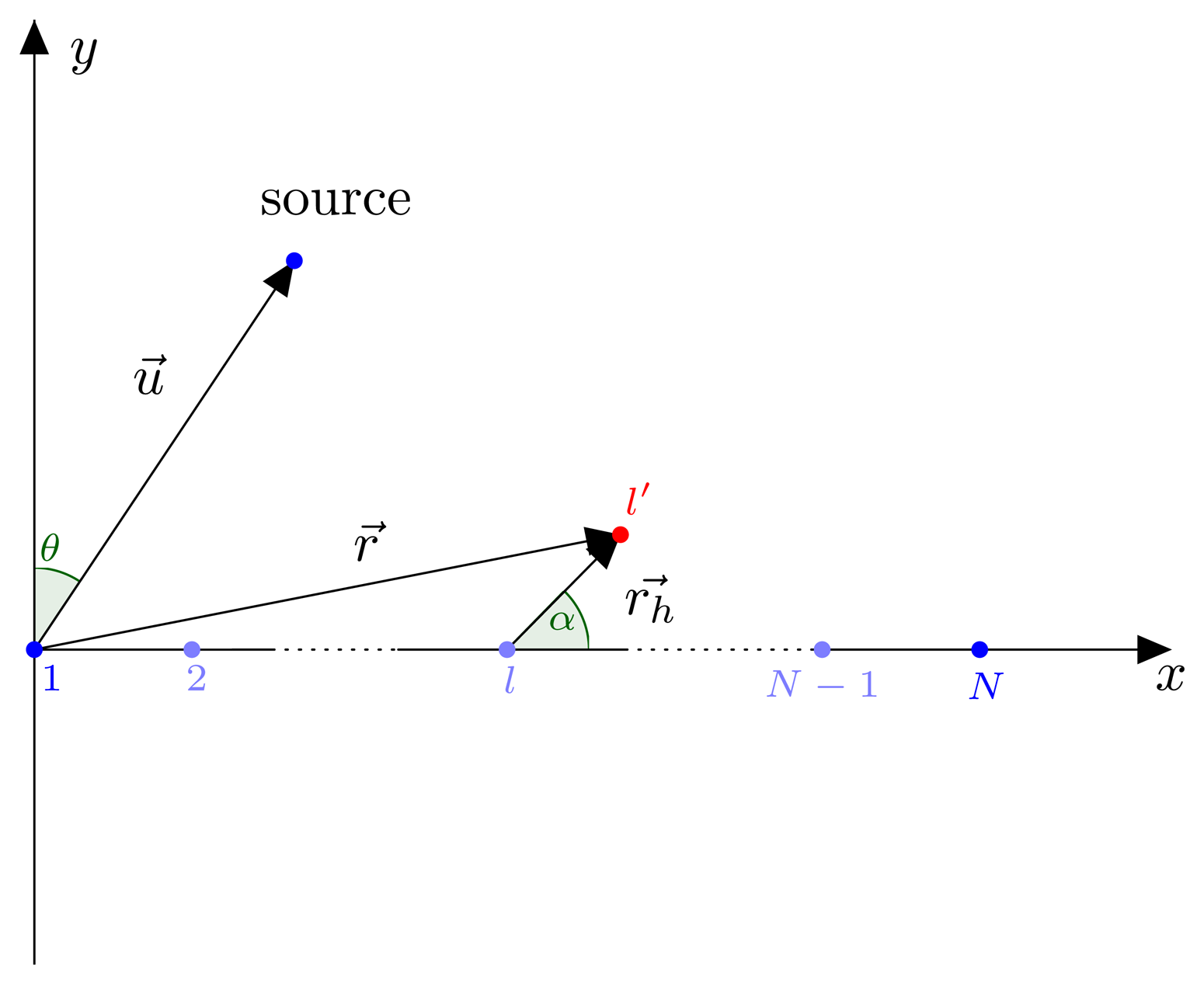
In this section, we assume that one of the sensor elements is displaced due to an unintentional movement of an element. Figure 1 depicts an array of N sensor elements, where the first sensor element is placed at the origin of the xy-plane and the other elements along the x-axis of this plane. The l-th sensor element is displaced by a vector with respect to its original position.
Denote and . The new coordinates of the displaced l-th sensor are given by r⃗ = [(l − 1)d + rh cos(α), rh sin(α)]. Define β = arg(r⃗) and r = ‖r⃗‖, such that . u⃗ is the unit vector with the same direction of the position vector of the source, which is located in the array's far field. The l-th row of the array manifold matrix then becomes .
4. Stochastic Collocation Method
In order to investigate the influence of a stochastic displacement of one of the sensor elements, we need stochastic simulation tools to characterize the statistical distribution of the DOAs due to the distribution of the random displacement vectors.
A Monte-Carlo simulation for such a task requires a large amount of realizations to accurately capture the statistics of the random process. Therefore, we apply the SCM proposed in [10] as a more effective way to rapidly model geometrical uncertainty, due to random variations of the array element positions.
4.1. One-Dimensional Stochastic Input
Assume that an input random variable X (in our case, e.g., the displacement in the x- or y-direction) is given. We want to determine the variation of the output Y = f(X) (in this paper, the DOA estimates), due to the statistical variation of X. The random variable X follows the cumulative distribution PX and probability density function dPX in the sample space Ω. To determine the statistics of Y, we rely on the Askey scheme [25] to approximate the transformation Y = f(X) by a polynomial expansion of order P.
An optimal expansion is obtained when the set of expansion polynomials forms a complete orthogonal basis in Ω with orthogonality relation:
In this case, the Cameron-Martin [26] convergence theorem ensures exponential convergence to the function Y = f(X) for P → ∞. In the remainder of the paper, we assume that the statistical variation of X follows a Gaussian distribution in the sample space Ω. Relying on the Askey scheme, we know that the probabilistic Hermite polynomials Hk(X) provide an optimal expansion for the normal Gaussian distribution [25].
To determine the unknown expansion coefficients , we apply Galerkin weighting to Equation (7) [27]:
We can approximate this integral by a Q-point Gauss-Hermite quadrature rule, being [28]:
4.2. Two-Dimensional Stochastic Input
We assume that the variation of the output Y = f(X1, X2) depends on two independent stochastic variables X1 and X2, respectively, in the sample space Ω1 and Ω2, respectively (e.g., a displacement in the x- and y-direction).
We first extend the GPoC expansion (7) to two dimensions. For Y = f(X1, X2), we obtain:
In the case that X1 and X2 are independent Gaussian distributed variables with zero mean and dispersions σ1 and σ2, respectively, we can rewrite Equation (12) as:
We approximate this integral by using cubature formulas for the plane with weight function e−r2 ([30,31]):
The cubature formulas that we have applied in this paper are those from [32] with Q = 44, de = 15, those from [33] with Q = 99, de = 21 and those from [33] with Q = 172, de = 31.
Given the exponential convergence of the polynomial expansions, for the two-dimensional expansion, we have to apply the KR-root-MUSIC algorithm only Q1 · Q2 times, when making use of the tensor rule Equation (13). Whereas, if we use the cubature formulas following Equation (16), we need to apply the KR-root-MUSIC algorithm Q times. Once we have estimated the DOAs in the quadrature points, the whole distribution can be obtained by applying the Monte-Carlo method to the computationally cheap polynomial expansion instead of to the DOA estimation algorithms.
5. Results
In all simulation examples below, the signal-to-noise ratio SNR (in dB) is denned as:
In order to validate the efficiency of the SCM method, we will provide several numerical examples. We first consider the case where the displacement vector is a constant vector. Next, we focus on the more general case where the x- and/or the y-coordinates of the displacement vector are random variables.
In Section 5.1, we investigate the influence on the DOA estimates obtained by root-MUSIC and KR-root-MUSIC for a displacement of one sensor element, in absence of noise. In Section 5.2, we use the SCM method to approximate the curves obtained in Section 5.1. In Section 5.3, we analyze the cdf for a displacement of the sensor element in one direction, for noisy data signals. In Section 5.4, we derive the GPoC expansion by means of the SCM method for a two-dimensional shift.
5.1. One Shifted Sensor Element: DOA Estimation in Absence of Noise
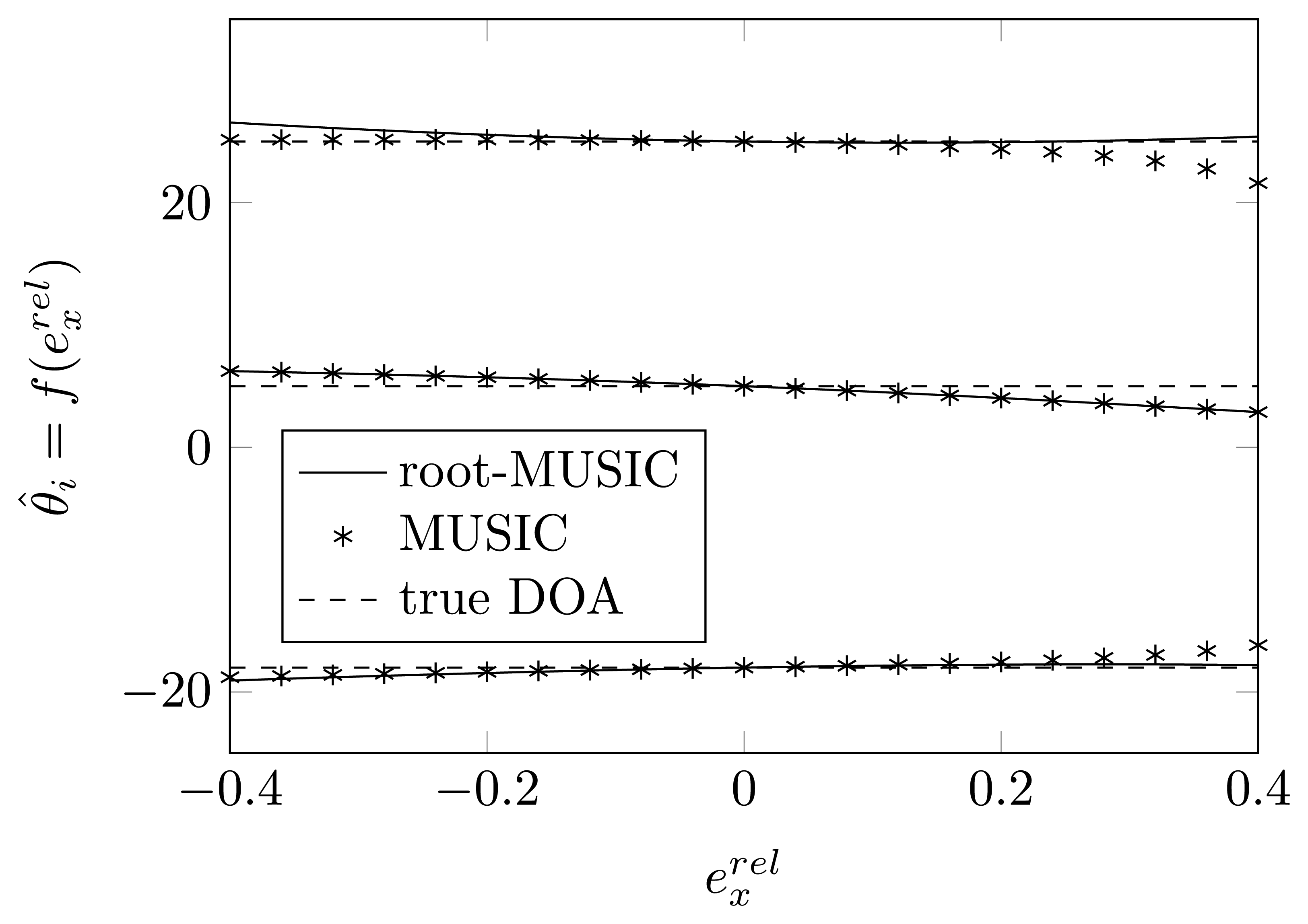
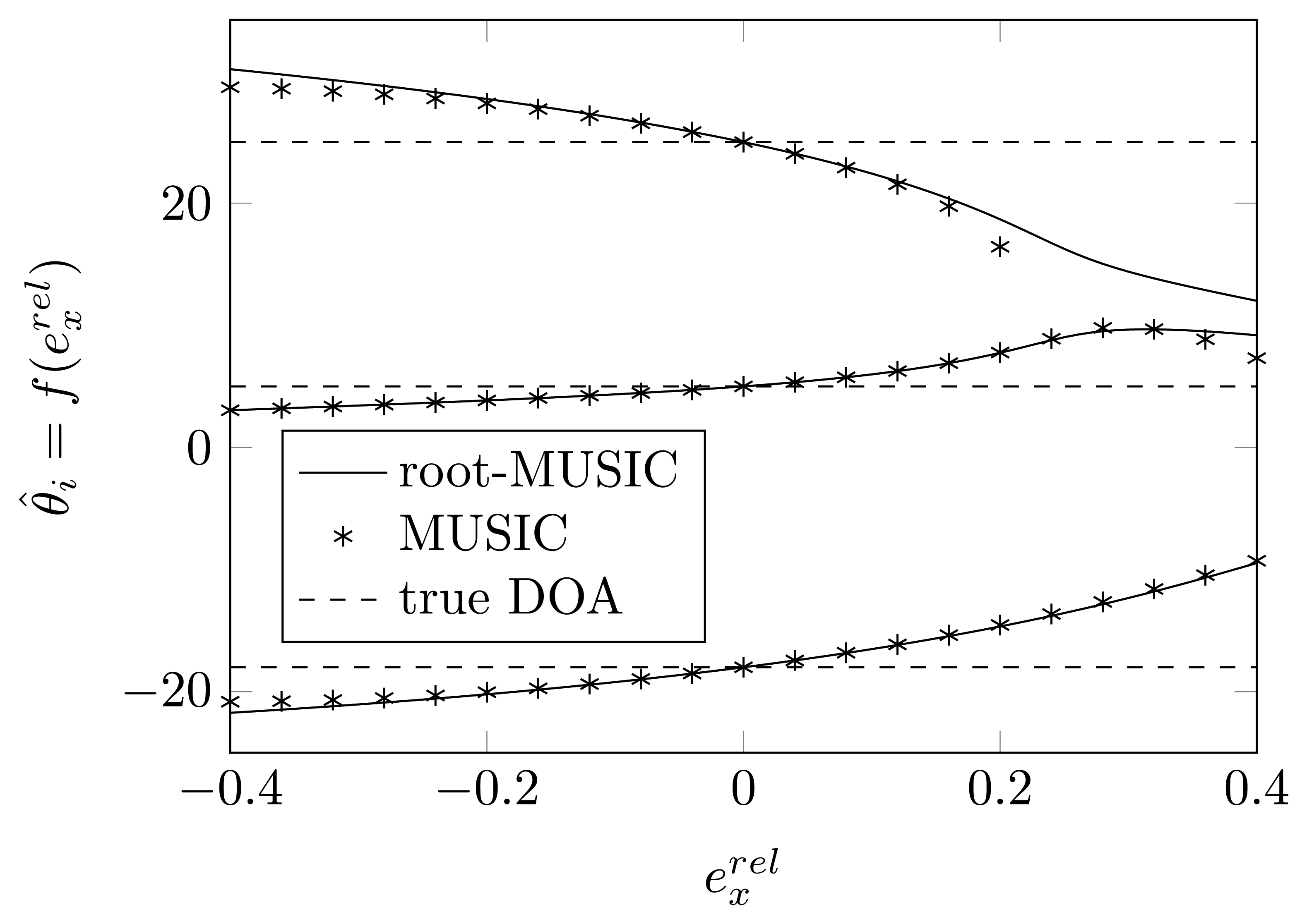
Consider the case of K = 3 sources and N = 4 sensor elements. The true DOAs are assumed to be [−18°, 5°, 25°]. We apply the synthetic signal generation procedure of Section 2.1 to generate a random source signal and use this signal vector throughout the simulations. We furthermore assume that no noise has been added to the impinging signal. We assume that one of the sensor elements has moved along the x-axis. For , being the relative displacement (with respect to the distance d between two sensor elements) of the sensor element, corresponds to coordinates [ , 0].
In Figures 2 and 3, we plot the estimated DOAs, as a function of for a relative displacement of each of the sensor elements for the root-MUSIC algorithm and the MUSIC algorithm. As a reference, the figures also show the true DOAs as dashed lines. We observe that even without any noise, the MUSIC algorithm is sensitive to a shift of one of the sensor elements and that if that shift is too large, in some cases, we do not find peaks in the MUSIC spectrum, such as in Figure 3 for . On the same figure, we observe that the root-MUSIC algorithm [24] estimates all DOAs, even in these cases where the conventional MUSIC algorithm does not find enough peaks. Furthermore, we observe that the DOAs estimated by the root-MUSIC algorithm and those estimated by the MUSIC algorithm are almost the same. The figures for a displacement of the first and fourth array element and those for a displacement of the second and third array element will almost be symmetric.
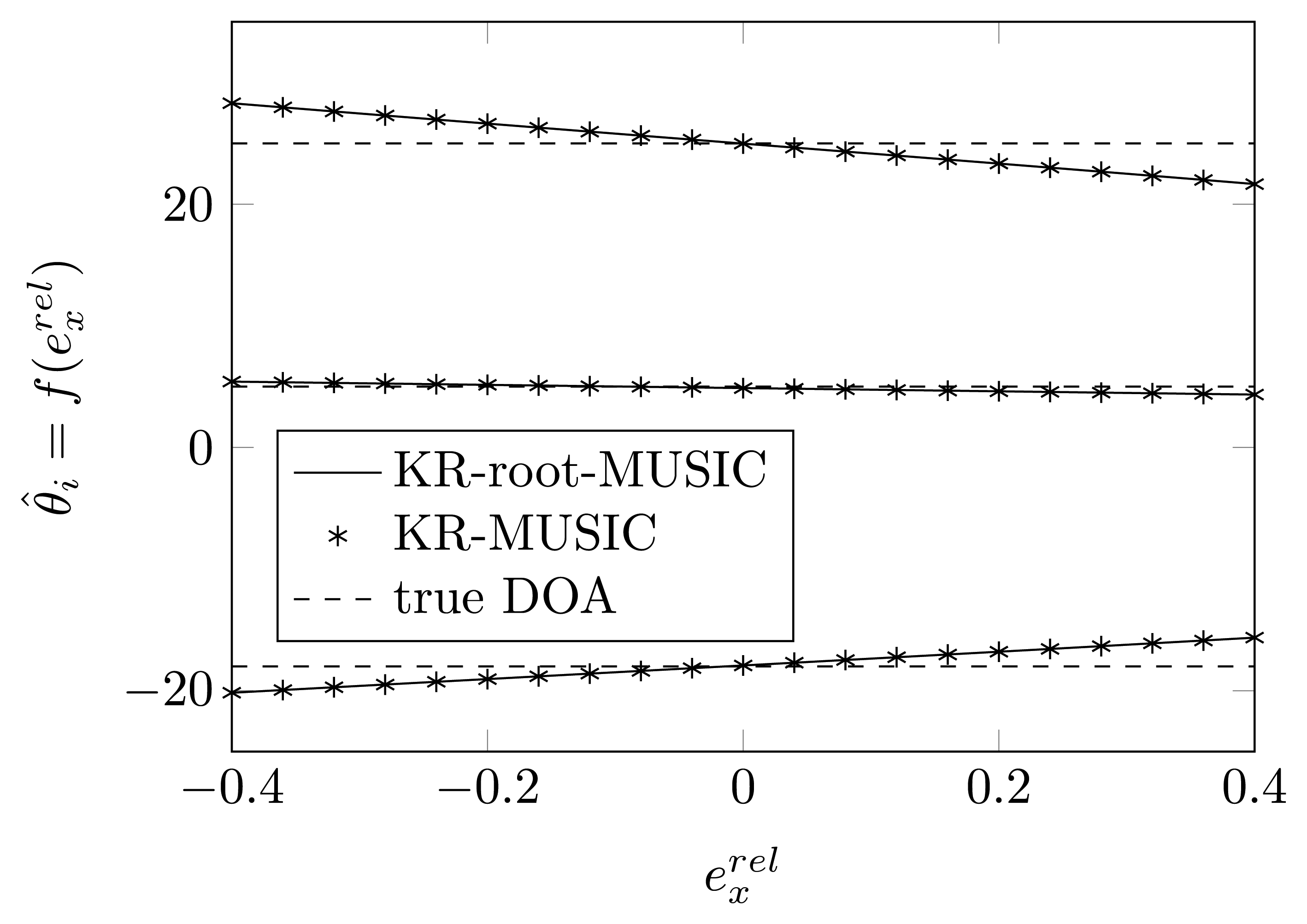
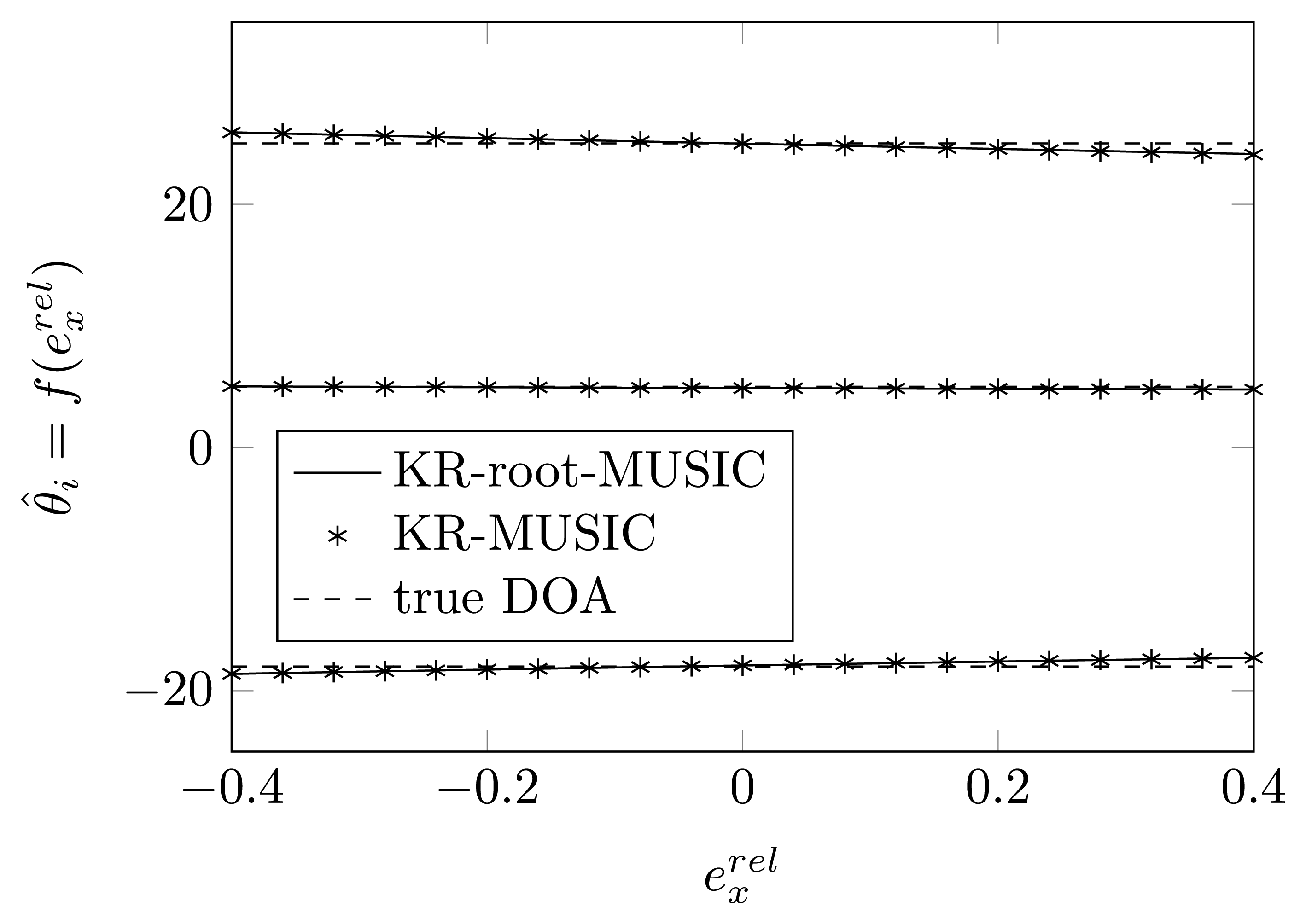
In Figures 4 and 5, we have plotted the estimated DOAs, as a function of , for a random relative displacement of the first and second sensor element for the KR-MUSIC and KR-root-MUSIC algorithm. In contrast to MUSIC, the KR-MUSIC algorithm is more robust to shifts in one of the sensor elements. The Khatri-Rao transformation expands the dimension of the vector on which we perform the SVD and the extracted noise subspace matrix. This increases the probability of finding K peaks. We also observe that in the KR-MUSIC case, the estimated curves are almost linear as a function of the shifts. Furthermore, we observe that DOAs estimated by using the KR-MUSIC algorithm are almost the same as those estimated by the KR-root-MUSIC algorithm.
5.2. One-Dimensional GPoC Expansion
In this section, we start from the same assumptions as in Section 5.1, concerning the impinging signal and the sensor array.
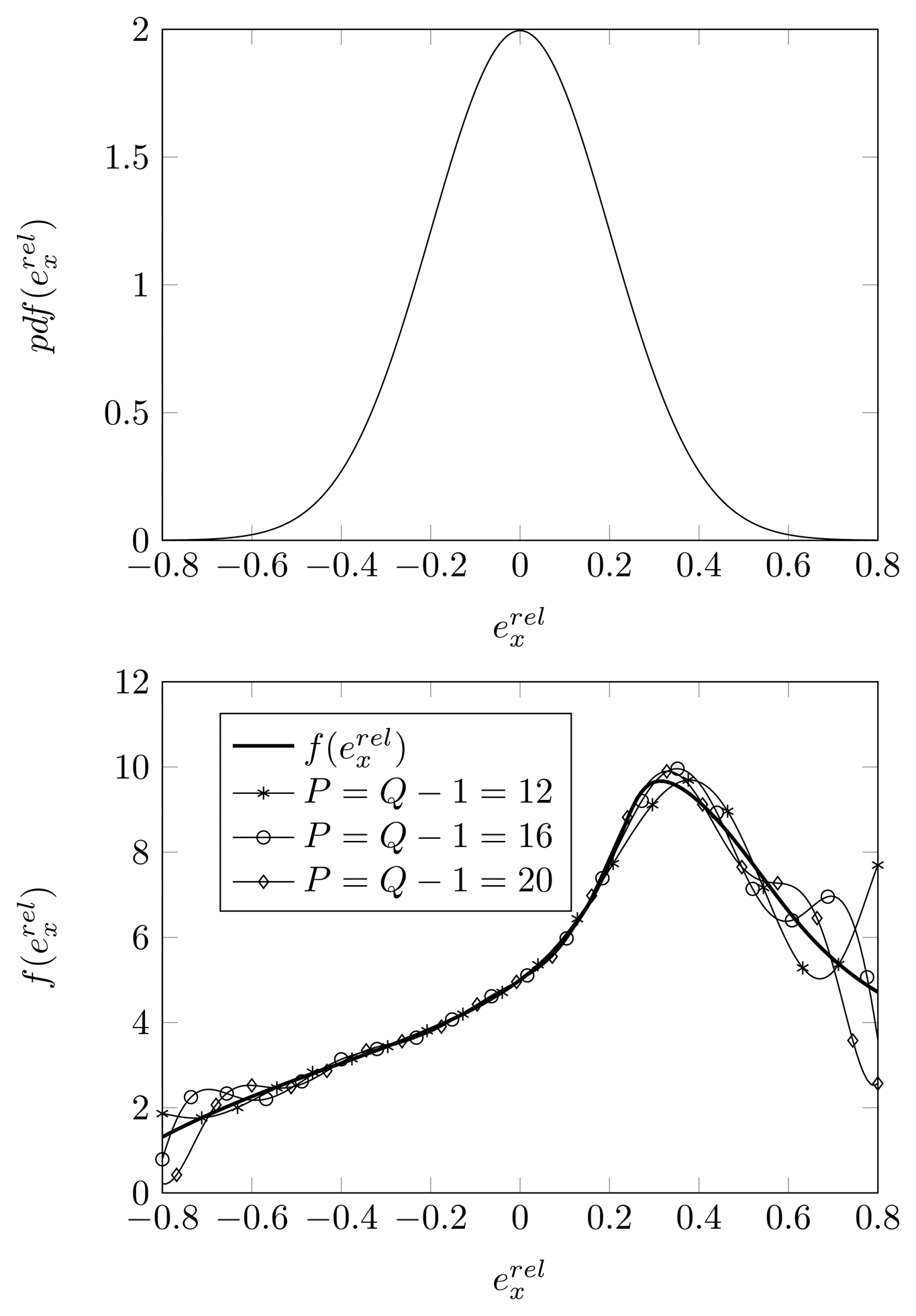
Let be the estimation of the second DOA (true DOAs = [−18°, 5°, 25°]) as a function of the relative displacement of the second sensor element along the x-axis . As plotted in the top figure of Figure 6, the relative displacement is assumed to be Gaussian distributed with dispersion σpl = 0.08. As outlined in Section 4, we therefore apply Hermite polynomials in the GPoC expansion of . We use the SCM method (with Q quadrature points and a polynomial expansion of order P = Q − 1) to determine the expansion coefficients for the GPoC expansion. In the bottom figure of Figure 6, we have plotted the function and the GPoC expansion of . We remark that, for between −0.16 and 0.16, all plotted curves coincide within 1%. We also observe that, if we make use of a higher expansion order for the polynomials, the GPoC expansions better approximate the curve representing . For a polynomial expansion of order 16, the GPoC curve coincides with the curve within 8% in the observed interval.
In Figure 7, we apply the SCM method with P = Q − 1 for Gaussian distributed with dispersion σpl = 0.2. We observe that, in the 95% confidence interval [−0.4,0.4] for , the GPoC based on the Hermite polynomials of order 12 or higher provides an accurate approximation for . However, beyond the 95% confidence interval, the Hermite polynomials rapidly oscillate, and they do not yield a good approximation for the curve.
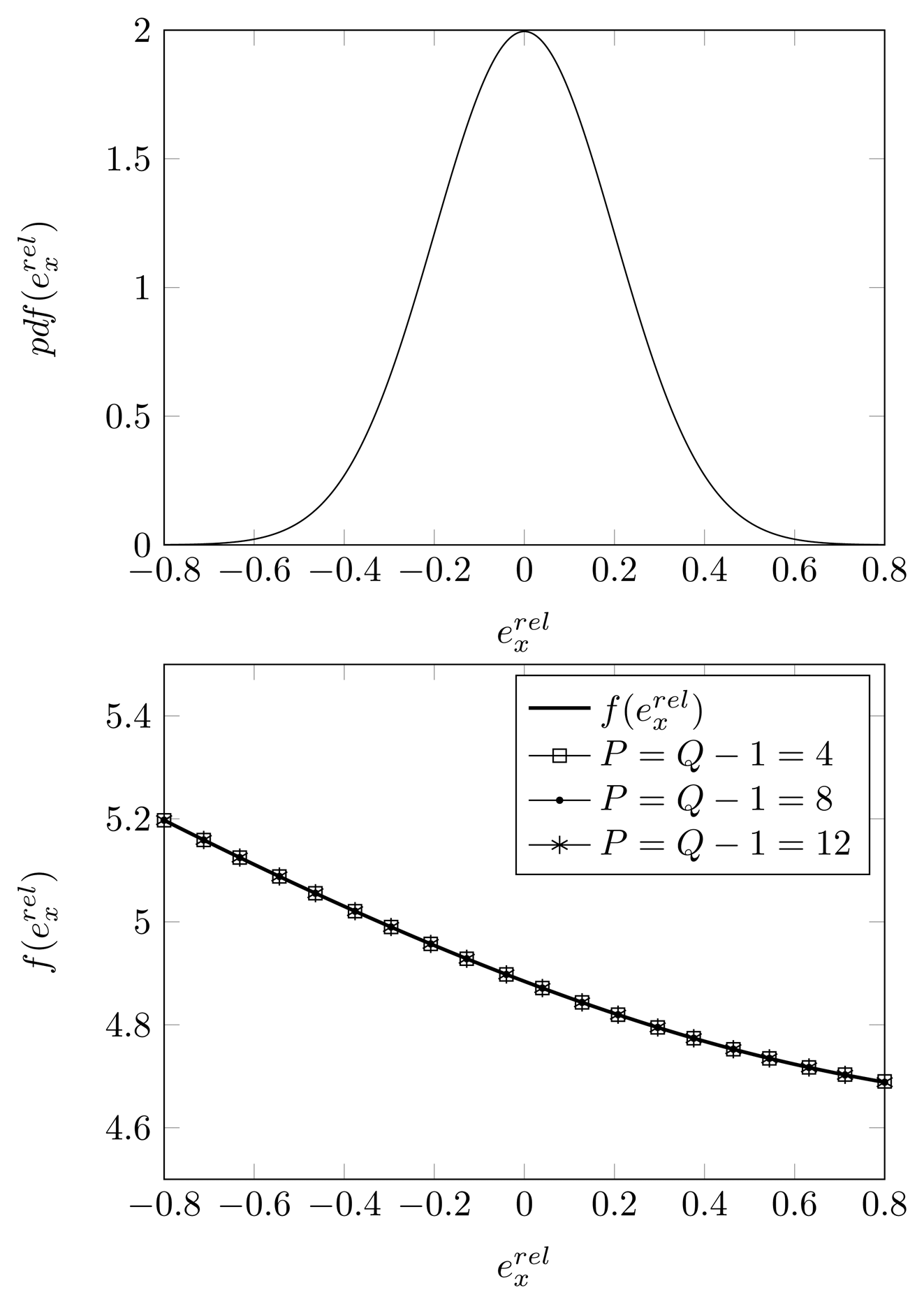
In Figure 8, we have made the same assumptions as in Figure 7, but we have estimated the DOA using the KR-root-MUSIC algorithm. The curves coincide, even when restricting the GPoC to only P = 4.
5.3. One Shifted Element: Statistical Distribution of DOA Estimates
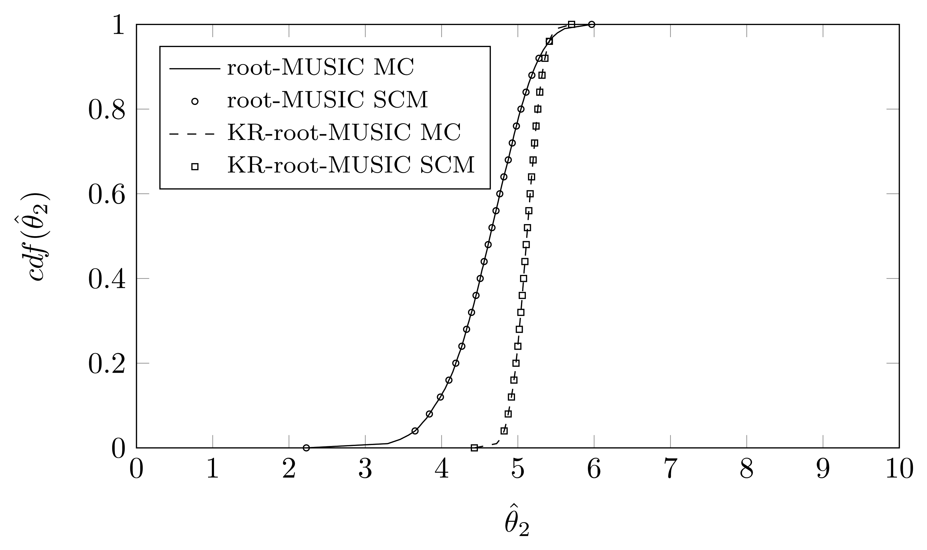
In this section, we again apply the synthetic signal generation procedure of Section 2.1 to generate a source signal. We construct an arbitrary complex Gaussian distributed noise vector v(t) = υR(t) + υI(t). υR(t) and υI(t) are both Gaussian distributed with zero mean and dispersion σ = 0.3 providing an SNR = 7.78 dB. Throughout the simulations, we use this source signal vector and noise vector. We also assume that the first sensor element is displaced along the x-axis and that the relative displacement is Gaussian distributed with zero mean and dispersion σpl = 0.12. To obtain the cdfs, we use two different methods: Monte-Carlo (MC) simulation and SCM. We carry out an MC simulation (where we vary ) with 10,000 realizations. The CPU-time to carry out this simulation equals about 126 s for the root-MUSIC algorithm and 157 s for the KR-root-MUSIC algorithm. The simulations were performed on a Dell Latitude E6520PC with an Intel(R) Core(TM)i5-2520M 2.5 GHz processor and 4 GB RAM. The MATLAB version used is 8.0.0.783 (R2012b).
We also apply the SCM theory for different values of the quadrature points Q and a polynomial expansion of Y of order P = Q − 1. We perform a two-sample Kolmogorov–Smirnov test (KS test) [34], to compare the samples obtained by the MC method with those obtained by the SCM method. The two-sample KS test verifies the null hypothesis that the two samples come from the same distribution. The test statistic is denned as:
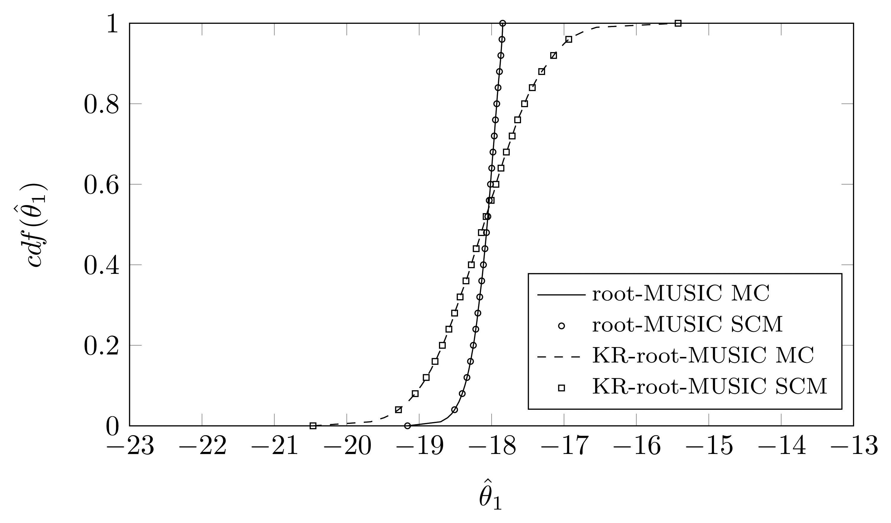
For the KR-root-MUSIC algorithm, both empirical distributions are the same for P = Q − 1 = 4. In Figures 9, 10 and 11, we have plotted the cdfs both obtained by the SCM method (with Q = 9 quadrature points and a polynomial expansion of order P = 8) and the MC method. We observe that, even for a small number of quadrature points, we see almost no difference between the curves obtained by the SCM theory and the curves obtained by MC simulation, as indicated by the true sample KS test. Moreover, for the first and third estimated DOA, the root-MUSIC algorithm estimates the DOA very accurately. For the estimation of the second DOA, however, the KR-root-MUSIC algorithm performs better.
5.4. Two-Dimensional Displacement of One Sensor Element
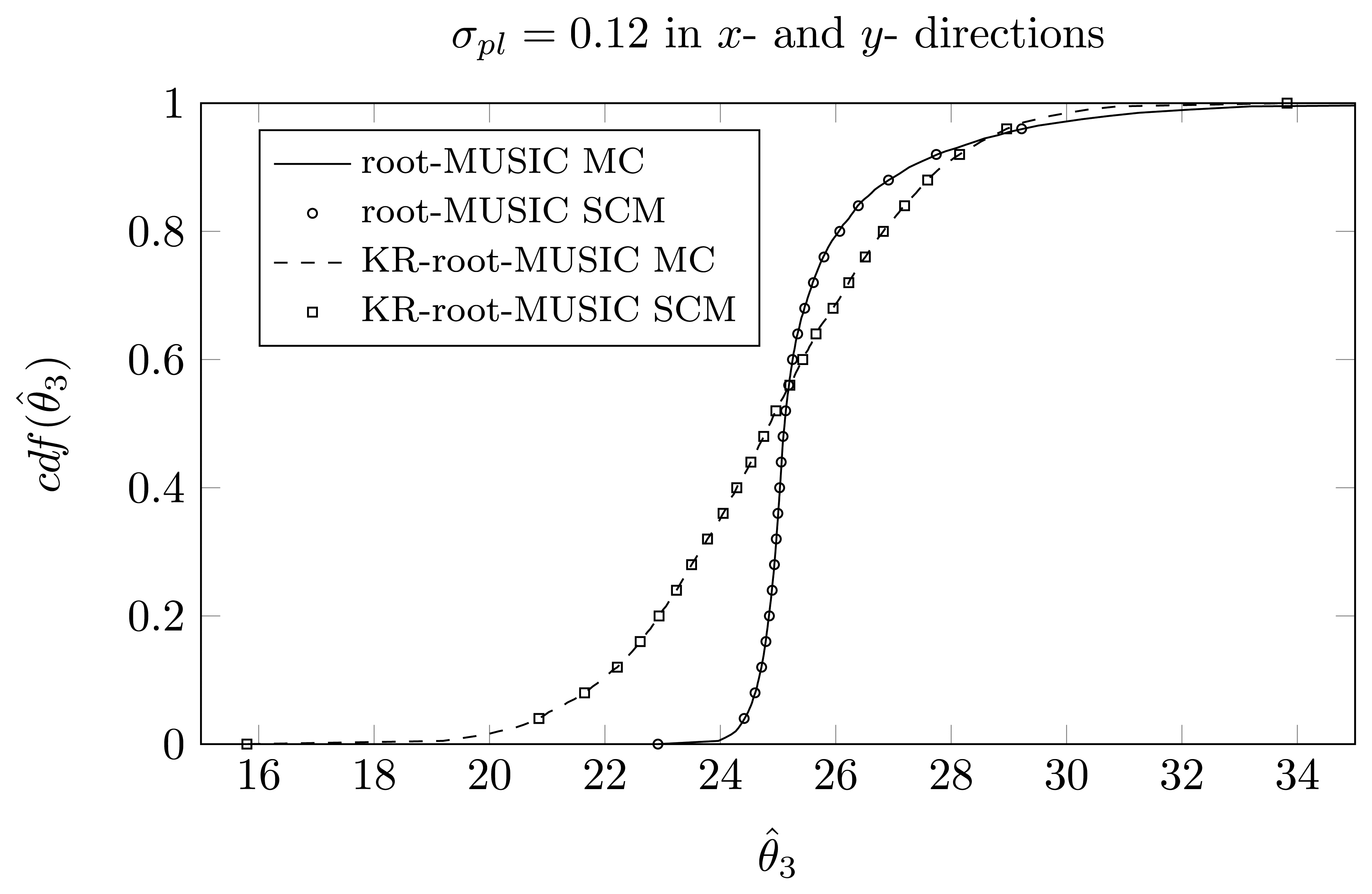
In this section, we assume that the first sensor element is displaced by (Figure 1). The relative displacements in both the x-direction and y-direction are independently Gaussian distributed, with zero mean and dispersion σpl. This means that the relative length of the displacement vector is Rayleigh distributed with mean and variance and that the argument of the displacement vector is uniformly distributed in [−π, π].
For the same impinging signal as in Section 5.3, we have plotted the cdfs of the different estimated DOAs, for σpl = 0.12. We have carried out an MC simulation with 10,000 realizations. The simulation time is about 128 s for the root-MUSIC algorithm and 157 s for the KR-root-MUSIC algorithm. We also apply the two-dimensional GPoC expansion (11) with degree P in both variables to obtain the cdfs for the DOAs. We calculate the weight coefficients using Q1 = Q2 = P − 1 quadrature points in the x- and y-directions using Equation (13). Tables 3 and 4 show the KS test to compare the samples obtained by the SCM method and the MC method. Furthermore, we compare this with the two-dimensional SCM theory that relies on the cubature formulas with Q = 44, Q = 99 and Q = 172, respectively, and with polynomial expansions of order P = 7, P = 10 and P = 15, respectively. The measured value of the KS test, which compares the samples of the MC method with those obtained with the cubature formulas, is also presented in Tables 3 and 4. Furthermore, the simulation times are shown in the last column of the tables. We observe that now, for the root-MUSIC algorithm, we need 14 quadrature points in each direction to satisfy the null hypothesis of the KS test (α = 0.05). Using cubature formulas, only for the estimates of the third DOA, 172 quadrature points are insufficient to satisfy the null hypothesis. For the KR-root-MUSIC algorithm, four quadrature points in each direction are sufficient. If we use cubature formulas, Q = 44 quadrature points are sufficient to satisfy the null hypothesis. We also observe that, using the SCM theory, the simulation time is reduced by a factor of about 20, and using the cubature formulas, we can reduce the simulation time by a factor of 56.
In Figures 12, 13 and 14, we have plotted the empirical cdf for the MC simulation and for the SCM method P = Q − 1 = 13. We observe that both curves almost coincide.
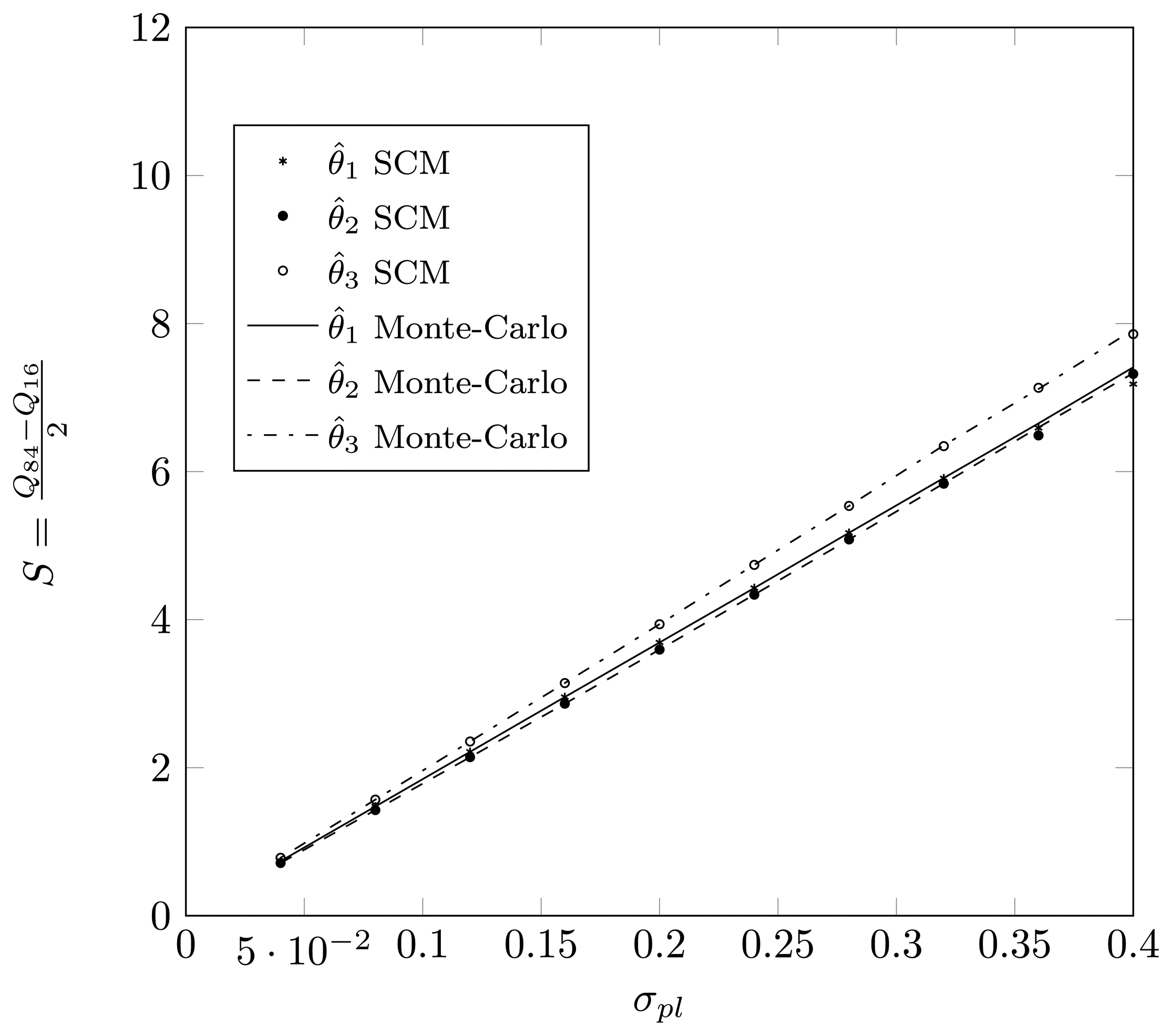
Define Qp as the p-th percentile of the estimated DOA, meaning that p% of the estimates for the true DOA are below Qp. Define , such that 68% of the estimates lie in an interval of length 2S around the true DOA. For a Gaussian distribution, the value S will correspond to the dispersion. In Figures 15 and 16, we have plotted the value S as a function of σpl for a two-dimensional displacement of the first sensor element. Again, we observe that the SCM method provides a good approximation for the estimates, both for the root-MUSIC algorithm as for the KR-root-MUSIC algorithm. Observe that for values σpl less than 0.4, the root-MUSIC yields better estimates for the first and third DOA than the KR-root-MUSIC algorithm. However, the KR-root-MUSIC estimates the second DOA better. We furthermore observe that, for the KR-root-MUSIC algorithm, the S-values are straight lines as a function Of σpl.
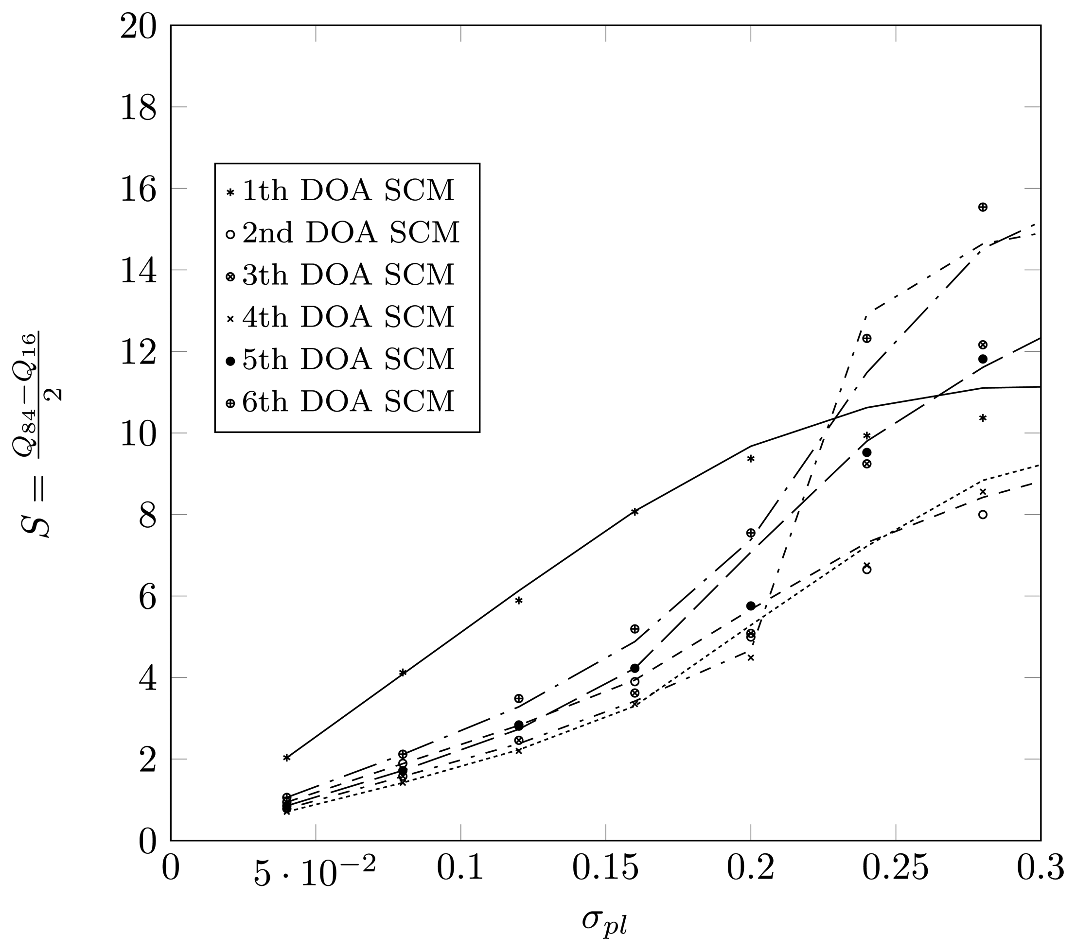
In Figure 17, we consider the (N,K) = (4,6) case with a displacement of the first sensor element and with the KR-root-MUSIC algorithm. The true DOAs to be estimated are [−65°, −40°, −20°, 10°, 25°, 42°]. Observe that, with the same array configuration as in Figure 16, we estimate twice as many DOAs. Looking at the , we observe that the KR-root-MUSIC algorithm finds the first estimate for θ̂1 = −65° with a large error, even for small values of σpl. The estimation error for the remainder of the DOAs starts to increase dramatically for values of σpl larger than 0.2.
6. Conclusions
In this paper, we have investigated the effect of a displacement of one of the sensor elements. We have applied the SCM formalism to efficiently predict the cdfs of the estimated DOAs, in the case that the relative displacement is Gaussian distributed. Comparison of the SCM method to the Monte-Carlo method demonstrates that SCM is an accurate method to predict the cdfs of the DOAs. For the one-dimensional case, the SCM method decreases the simulation time by a factor of more than 100. For the two-dimensional case and using cubature formulas, we can reduce the simulation time by a factor of 56. In the future, we will extend the applied method to array configurations in which more sensor elements are displaced. Moreover, the SCM will be applied to other DOA estimation algorithms and for other array configurations. The flexibility and non-intrusive character of the proposed method only requires that DOA-estimates need to be computed in the quadrature points, by use of the appropriate algorithm.
Acknowledgments
This research was partially funded by the Inter-University Attraction Poles Program initiated by the Belgian Science Policy Office.
Author Contributions
All authors contributed extensively to the study presented in this manuscript. Veronique Inghelbrecht designed the main idea, carried out the simulation, interpreted the results and wrote the paper. Jo Verhaevert, Hendrik Rogier and Tanja Van Hecke supervised the main idea and edited the manuscript. They provided many valuable suggestions to this study: Jo Verhaevert and Hendrik Rogier especially in the domain of sensors; Tanja Van Hecke especially in the domain of statistical analysis.
Conflicts of Interest
The authors declare no conflict of interest.
References
- Ma, W.K.; Hsieh, T.H.; Chi, C.Y. DOA estimation of quasi-stationary signals with less sensors than sources and unknown spatial noise covariance: A Khatri-Rao subspace approach. IEEE Trans. Signal Process. 2010, 58, 2168–2180. [Google Scholar]
- Brown, G.; McClellan, J. Performance bound analysis of a hybrid array. IEEE Trans. Signal Process. 1996, 44, 74–82. [Google Scholar]
- Tam, P.; Wong, K. Cramer-Rao bounds for direction finding by an acoustic vector sensor under nonideal gain-phase responses, noncollocation, or nonorthogonal orientation. IEEE Sens. J. 2009, 9, 969–982. [Google Scholar]
- Tam, P.; Wong, K. An hybrid Cramer-Rao bound in closed form for direction-of-arrival estimation by an “acoustic vector sensor” with gain-phase uncertainties. IEEE Trans. Signal Process. 2014, 62, 2504–2015. [Google Scholar]
- Friedlander, B.; Weiss, A. Effects of model errors on waveform estimation using the MUSIC algorithm. IEEE Trans. Signal Process. 1994, 42, 147–155. [Google Scholar]
- Lo, J.; Marple, S. Observability conditions for multiple signal direction finding and array sensor localization. IEEE Trans. Signal Process. 1992, 40, 2641–2650. [Google Scholar]
- Ratnarajah, T.; Manikas, A. An H∞ approach to mitigate the effects of array uncertainties on the MUSIC algorithm. IEEE Signal Process Lett. 1998, 5, 185–188. [Google Scholar]
- Viberg, M.; Swindlehurst, A. Analysis of the combined effects of finite sampes and model errors on array processing performance. IEEE Trans. Signal Process. 1994, 42, 3073–3083. [Google Scholar]
- Weiss, A.; Friedlander, B. IEEE Trans. Signal Process. 1996, 44, 1024–1027.
- Rogier, H.; Boeykens, F. An efficient technique based on polynomial chaos to model the uncertainty in resonance frequency of textile antennas due to bending. IEEE Trans. Antennas Propag. 2014, AP-62, 1253–1260. [Google Scholar]
- Friedlander, B. A sensitivity analysis of the MUSIC algorithm. IEEE Trans. Acoust. Speech Signal Process. 1990, 38, 1740–1751. [Google Scholar]
- Weiss, A.; Friedlander, B. Effects of modeling errors on the resolution threshold of the Music algorithm. IEEE Trans. Signal Process. 1994, 42, 1519–1526. [Google Scholar]
- Chevalier, P.; Ferreol, A. On the virtual array concept for the fourth-order direction finding problem. IEEE Trans. Signal Process. 1999, 47, 2592–2595. [Google Scholar]
- Pal, P.; Vaidyanathan, P. Nested arrays: A novel approach to array processing with enhanced degrees of freedom. IEEE Trans. Signal Process. 2010, 58, 4167–4181. [Google Scholar]
- Sidiropoulos, N.; Bro, R. Parallel factor analysis in sensor array processing. IEEE Trans. Signal Process. 2000, 48, 2377–2388. [Google Scholar]
- Feng, D.; Bao, M.; Ye, Z.; Guan, L.; Li, X. A novel wideband DOA estimator based on Khatri-Rao subspace approach. Signal Process. 2011, 91, 2415–2419. [Google Scholar]
- Valaee, S.; Kabal, P. Wideband array processing using a two-sided correlation transformation. IEEE Trans. Signal Process. 1995, 43, 160–172. [Google Scholar]
- He, Z.Q.; Shi, Z.P.; Huang, L.; So, H. Underdetermined DOA estimation for wideband signals using robust sparse covariance fitting. IEEE Signal Process. Lett. 2013, 22, 435–439. [Google Scholar]
- He, Z.Q.; Shi, Z.P.; Huang, L. Covariance sparsity-aware DOA estimation for nonuniform noise. Digit. Signal Process. 2014, 28, 75–81. [Google Scholar]
- Cao, M.Y.; Huang, L.; Qian, C.; Xue, J.J.; So, H. Underdetermined DOA estimation of quasi-stationary signal via Khatri-Rao structure for uniform circular array. Signal Process. 2015, 106, 41–48. [Google Scholar]
- Guo, X.; Li, B.; Chu, L.; Wang, D. Near-Field source localization in complex indoor environment uniform circular array. Proceedings of IEEE China Summit & International Conference on Signal and Information Processing, Xi'an, China, 9–13 July 2014; pp. 412–415.
- Palanisamy, P.; Kishore, C. 2-D DOA estimation of quasi-stationary signals based on Khatri-Rao subspace approach. Proceedings of IEEE-International Conference on Recent Trends in Information Technology, Chennai, India, 3–5 June 2011; pp. 798–803.
- Chan, F.; So, H.; Huang, L.; Huang, L.T. Underdetermined direction-of-departure and direction-of-arrival estimation in bistatic multiple-input multiple-output radar. Signal Process. 2014, 104, 284–290. [Google Scholar]
- Barabell, A. Improving the resolution performance of eigenstructured-based direction-finding algorithms. Proceedings of IEEE International Conference on ICASSP '83 Acoustics, Speech, and Signal Processing, Boston, MA, USA, 14–16 April 1983; pp. 336–339.
- Xiu, D. Fast numerical methods for stochastic computations: A review. Commun. Comput. Phys. 2009, 5, 242–272. [Google Scholar]
- Cameron, R.; Martin, W. Transformations of Wiener integrals under translations. Ann. Math. 1944, 45, 386–396. [Google Scholar]
- De Staelen, R.; Crevecoeur, G. A sensor sensitivity and correlation analysis through polynomial chaos in the EEG problem. IMA J. Appl. Math. 2014, 79, 163–174. [Google Scholar]
- Eldred, M.S.; Webster, C.G. Evaluation of non-intrusive approaches for Wiener-Askey generalized polynomial chaos. Proceedings of 49th AIAA/ASME/ASCE/AHS/ASC Structures, Structural Dynamics, and Materials Conference, Schaumburg, IL, USA, 7–10 April 2008.
- Caflisch, R. Monte Carlo and quasi-Monte Carlo methods. Acta Numer. 1998, 7, 1–49. [Google Scholar]
- Bagci, H.; Yucel, A.; Hesthaven, J.; Michielssen, E. A fast Stroud-based collocation method for statistically characterizing EMI/EMC phenomena on complex platforms. IEEE Trans. Electromagn. Compat. 2009, 51, 301–311. [Google Scholar]
- Cools, R. An encyclopaedia of cubature formulas. J. Complex. 2003, 19, 445–453. [Google Scholar]
- Stroud, A. Approximate Calculation of Multiple Integrals; Prentice-Hall: Upper Saddle River, NJ,USA, 1971. [Google Scholar]
- Cools, R.; Pluym, L.; Laurie, D. Cubpack++: A C++ package for automatic two-dimensional cubature. ACM Trans. Math. Softw. (TOMS) 1997, 23, 1–15. [Google Scholar]
- Marsaglia, G.; Tsang, W.; Wang, J. Evaluating Kolmogorov's distribution. J. Stat. Softw. 2003, 8, 1–4. [Google Scholar]


| root-MUSIC, σpl = 0.12 | |||||
|---|---|---|---|---|---|
| Dn,n′ for | |||||
| P | Q | θ1 | θ2 | θ3 | time |
| 4 | 5 | 0.0088 | 0.0004 | 0.0190 | 0.16 s |
| 8 | 9 | 0.0002 | 0.0002 | 0.0006 | 0.17 s |
| 12 | 13 | 0.0002 | 0.0001 | 0.0005 | 0.25 s |
| 16 | 17 | 0.0001 | 0.0001 | 0.0002 | 0.39 s |
| KR-root-MUSIC, σpl = 0.12 | |||||
|---|---|---|---|---|---|
| Dn,n′ for | |||||
| P | Q | θ1 | θ2 | θ3 | time |
| 4 | 5 | 0.0002 | 0.0001 | 0.0003 | 0.09 s |
| 8 | 9 | 0.0001 | 0.0001 | 0.0001 | 0.33 s |
| 12 | 13 | 0.0001 | 0.0001 | 0.0001 | 0.36 s |
| 16 | 17 | 0.0001 | 0.0001 | 0.0001 | 0.55 s |
| root-MUSIC, σpl = 0.12 | |||||
|---|---|---|---|---|---|
| Dn,n′ for | |||||
| P1 = P2 | Q1 = Q2 | θ1 | θ2 | θ3 | time |
| 7 | 8 | 0.0251 | 0.0039 | 0.0731 | 4.14 s |
| 10 | 11 | 0.0102 | 0.0025 | 0.0255 | 5.63 s |
| 13 | 14 | 0.0038 | 0.0033 | 0.0112 | 6.40 s |
| P | Q | θ1 | θ2 | θ3 | time |
| 7 | 44 | 0.0134 | 0.0052 | 0.0486 | 0.76 s |
| 10 | 99 | 0.0061 | 0.0021 | 0.0309 | 1.54 s |
| 15 | 172 | 0.0044 | 0.0021 | 0.0219 | 2.22 s |
| KR-root -MUSIC, σpl = 0. 12 | |||||
|---|---|---|---|---|---|
| Dn,n′ for | |||||
| P1 = P2 | Q1 = Q2 | θ1 | θ2 | θ3 | time |
| 7 | 8 | 0.0002 | 0.0002 | 0.0002 | 4.74 s |
| 10 | 11 | 0.0001 | 0.0002 | 0.0001 | 6.01s |
| 13 | 14 | 0.0001 | 0.0001 | 0.0001 | 7.33 s |
| P | Q | θ1 | θ2 | θ3 | time |
| 7 | 44 | 0.0002 | 0.0002 | 0.0002 | 0.83 s |
| 10 | 99 | 0.0003 | 0.0003 | 0.0004 | 1.62 s |
© 2014 by the authors; licensee MDPI, Basel, Switzerland. This article is an open access article distributed under the terms and conditions of the Creative Commons Attribution license ( http://creativecommons.org/licenses/by/3.0/).
Share and Cite
Inghelbrecht, V.; Verhaevert, J.; Van Hecke, T.; Rogier, H. The Influence of Random Element Displacement on DOA Estimates Obtained with (Khatri–Rao-)Root-MUSIC. Sensors 2014, 14, 21258-21280. https://doi.org/10.3390/s141121258
Inghelbrecht V, Verhaevert J, Van Hecke T, Rogier H. The Influence of Random Element Displacement on DOA Estimates Obtained with (Khatri–Rao-)Root-MUSIC. Sensors. 2014; 14(11):21258-21280. https://doi.org/10.3390/s141121258
Chicago/Turabian StyleInghelbrecht, Veronique, Jo Verhaevert, Tanja Van Hecke, and Hendrik Rogier. 2014. "The Influence of Random Element Displacement on DOA Estimates Obtained with (Khatri–Rao-)Root-MUSIC" Sensors 14, no. 11: 21258-21280. https://doi.org/10.3390/s141121258
APA StyleInghelbrecht, V., Verhaevert, J., Van Hecke, T., & Rogier, H. (2014). The Influence of Random Element Displacement on DOA Estimates Obtained with (Khatri–Rao-)Root-MUSIC. Sensors, 14(11), 21258-21280. https://doi.org/10.3390/s141121258