Self-Learning Variable Structure Control for a Class of Sensor-Actuator Systems

Abstract
: Variable structure strategy is widely used for the control of sensor-actuator systems modeled by Euler-Lagrange equations. However, accurate knowledge on the model structure and model parameters are often required for the control design. In this paper, we consider model-free variable structure control of a class of sensor-actuator systems, where only the online input and output of the system are available while the mathematic model of the system is unknown. The problem is formulated from an optimal control perspective and the implicit form of the control law are analytically obtained by using the principle of optimality. The control law and the optimal cost function are explicitly solved iteratively. Simulations demonstrate the effectiveness and the efficiency of the proposed method.1. Introduction
With the development of mechatronics, automatic systems consisting of sensors for perception and actuators for action are more and more widely used in applications [1–4]. Besides the proper choices of sensors and actuators and an elaborate fabrication of mechanical structures, the control law design also plays a crucial role in the implementation of automatic systems especially for those with complicated dynamics. For most mechanical sensor-actuator systems, it is possible to model them in Euler-lagrange equations [4,5]. In this paper, we are concerned with the sensor-actuator systems modeled by Euler-lagrange equations.
Due to the importance of Euler-lagrange equations in modeling many real sensor-actuator systems, much attention has been paid to the control of such kind systems. According to the type of constraints, the Euler-lagrange system can be categorized into Euler-lagrange system without nonholonomic constraints (e.g., fully-actuated manipulator [6,7], omni-directional mobile robot [8]), and the system subject to nonholonomic constraint [9] (e.g., the cart-pole system [10], the under-actuated multiple body system [11]). For Euler-lagrange system without nonholonomic constraints, the dimension of inputs are often equal to the dimension of output and the system are often able to be transformed into a double integrator system by employing feedback linearization [12]. Other methods, such as control Lyapunov function method [13], passivity based method [14], optimal control method [15], etc., are also successfully applied to the control of Euler-lagrange system without nonholonomic constraints. In contrast, as the dimension of inputs is lower than that of outputs, it is often impossible to directly transform the Euler-lagrange system subject to nonholonomic constraints to a linear system and thus feedback linearization fails to stabilize the system. To tackle the difficulty, variable structure control based method [16], backstepping based control [17], optimal control based method [18], discontinuous control method [19], etc., are widely investigated and some useful design procedures are proposed. However, due to the inherent nonlinearity and nonholonomic constraints, most existing methods [16–19] are strongly model dependent and the performance are very sensitive to model errors. Inspired by the success of human operators for the control of Euler-lagrange systems, various intelligent control strategies, such as fuzzy logic [20], neural networks [21], evolutionary algorithms [22], to name a few of them, are proposed to solve the control problem of of Euler-lagrange systems subject to nonholonomic constraints. As demonstrated by extensive simulations, these type of strategies are indeed effective to the control of Euler-lagrange systems subject to nonholonomic constraints. However, rigorous proof on the stability are difficult for this type of methods and there may exist some initializations of the state, from which the system cannot be stabilized.
In this paper, we propose a self-learning control method applicable to Euler-lagrange systems. In contrast to existing work on intelligent control of Euler-lagrange systems, the stability of the close loop system with the proposed method is proven in theory. On the other hand, different from model based design strategies, such as backstepping based design [17], variable structure based design [16], etc., the proposed method does not require information of the model parameters and therefore is a model independent method. We formulate the problem from an optimal control perspective. In this framework, the goal is to find the input sequence to minimize the cost function defined on infinite horizon under the constraint of the system dynamics. The solution can be found by solving a Bellman equation according to the principle of optimality [23]. Then an adaptive dynamic programming strategy [24–26] is utilized to numerically solve the input sequence in real time.
The remainder of this paper is organized as follows: in Section 2, preliminaries on Euler-lagrange systems and variable structure control are given briefly. In Section 3, the problem is formulated as a constrained optimization problem and the critic model and the action model are employed to approximate the optimal mappings. The control law is then derived in Section 4. In Section 5, simulations are given to show the effectiveness of the proposed method. The paper is concluded in Section 6.
2. Preliminaries on Variable Structure Control of the Sensor-Actuator System
In this paper, we are concerned with the following sensor-actuator system in the Euler-Lagrange form,
As an effective design strategy, variable structure control finds applications in many different type of control systems including the Euler-Lagrange system. The method stabilizes the dynamics of a nonlinear system by steering the state to a elaborately designed sliding surface, on which the state inherently evolves towards the zero state. Particularly for the system (2), we define s = s(x1,x2) as follows:
About the Euler-Lagrange Equation (1) for modeling sensor-actuator systems, we have the following remark:
Remark 1 In this paper, we are concerned with the class of sensor-actuator systems modeled by the Euler-Lagrange Equation (1). Actually, the dynamics of mechanical systems can be described by the Euler-Lagrange equation according to the rigid body mechanics [4,5], which is essentially equivalent to Newton's laws of motion. Therefore, mechanical sensor-actuator system can be modeled by Equation (1). In this regard, the Euler-Lagrange equation employed in the paper models a general class of sensor-actuator systems.
3. Problem Formulation
Without losing generality, we stabilize the system (1) by steering it to the sliding surface s = 0 with s defined in Equation (3). Different from existing model based design procedures, we design a self-learning controller, which does not require accurate knowledge about D(q), C(q,q̇) and ϕ(q) in Equation (1). In this section, we formulate such a control problem from the optimal control perspective.
In this paper, we set the origin as the desired operating point, i.e., we consider the problem of controlling the state of the system (1) to the origin. For the case with other desired operating points, the problem can be equivalently transformed to the one with the origin as the operating point by shifting the coordinates. At each sampling period, the norm of s = c0x1 + x2, which measures the distance from the desired sliding surface s = 0, can be used to evaluate the one step performance. Therefore, we define the following utility function associated with the one-step cost at the ith sampling period,
Remark 2 There are infinitely many decision variables, which are u(0), u(1), …, u(∞), in the optimization problem in Equation (7). Therefore, this is an infinite dimensional problem. It cannot be solved directly using numerical methods. Conventionally, such kind of problem is often solved by using a finite dimensional approximation [27]. In addition, note that the dynamic model of the system appears in the optimization problem in Equation (7) and it will also show up in the finite dimensional relaxation of the problem, which means the resulting solution requires model information and thus is also model-dependent. In contrast, in this paper we investigate the model-independent variable structure control of sensor-actuator systems on the infinite time horizon.
4. Model-Free Control of the Euler-Lagrange System
In this section, we present the strategy to solve the constrained optimization problem efficiently without knowing the model information of the chaotic system. We first investigate the optimality condition of Equation (7) and present an iterative procedure to approach the analytical solution. Then, we analyze the convergence of the iterative procedure and the stability with the derived control strategy.
4.1. Optimality Condition
Denoting J* the optimal value to the optimization problem in Equation (7), i.e.,
According to the principle of optimality [23], the solution of Equation (7) satisfy the following Bellman equation:
Define the Bellman operator relative to function h(z) as follows
Then, the optimality condition in Equation (10) can be simplified into the following with the Bellman operator,
Note that the function Uk is implicitly included in the Bellman operator. The Equation (12) constitutes the optimality condition for problem in Equation (7). It is difficult to solve the explicit form of J* analytically from Equation (9). However, it is possible to get the solution by iterations. We use the following iterations to solve J*,
The control action keeps constant in the duration between the kth and the k + 1th step, i.e., u*(t) = for kτ ≤ t < (k + 1)τ. can be obtained from Equation (9) based on Equation (13),
4.2. Approximating the Action Mapping and the Critic Mapping
In the previous sections, the iteration (13) is derived to calculate J* and the optimization (14) is obtained to calculate the control law. The iteration to approach J* and the optimization to derive u* have to be run in every time step in order to obtain the most up-to-date values. Inspired by the learning strategies widely studied in artificial intelligence [26,28], a learning based strategy is used in this section to facilitate the processing. After a enough long time, the system is able to memorize the mapping of J* and the mapping of u*. After this learning period, there will be no need to repeat any iterations or optimal searching, which will make the strategy more practical.
Note that the optimal cost J* is a function of the initial state. Counting the cost from the current time step, J* can also be regarded as a function of both the current state and the optimal action at current time step according to Equation (10). Therefore, ĵ(n), the approximation of J*, can also be regarded as a function relative to the current state and the current optimal input. As to the optimal control action u*, it is a function of the current state. Our goal in this section is to obtain the mapping from the current state and the current input to ĵ (n) and the mapping from the current state to the optimal control action u* using parameterized models, denoted as the critic model and the action model, respectively. Therefore, we can write the critic model and the action model as Jn( xn, Wc) and (xn, Wa) respectively, where Wc is the parameters of the critic model and Wa is the parameters of the action model.
In order to train the critic model with the desired input-output correspondence, we define the following error at time step n + 1 to evaluate the learning performance,
Note that Bĵ(n) is the desired value of ĵ(n + 1) according to Equation (13). Using the back-propagation rule, we get the following rule for updating the weight Wc of the critic model,
As to the action model, the optimal control u* in Equation (14) is the one that minimizes the cost function. Note that the possible minimum cost is zero, which corresponds to the scenario with the state staying inside the desired bounded area. In this regard, we define the action error as follows,
Then, similar to the update rule of Wc for the critic model, we get the following update rule of Wa for the action model,
Equations (16) and (18) update the critic model and the action model progressively. After Wc and Wa have learnt the model information by learning for a long enough time, their values can be fixed at the one obtained at the final step and no further learning is required any longer, which is in contrast to Equation (14) requiring to solve an optimization problem even after a long enough time.
5. Simulation Experiment
In this section, we consider the simulation implementation of the proposed control strategy. The dynamics given in Equation (1) model a wide class of sensor-actuator systems. Particularly, to demonstrate the effectiveness of the proposed self-learning variable structure method, we apply it to the stabilizations of a typical benchmark system: the cart-pole system.
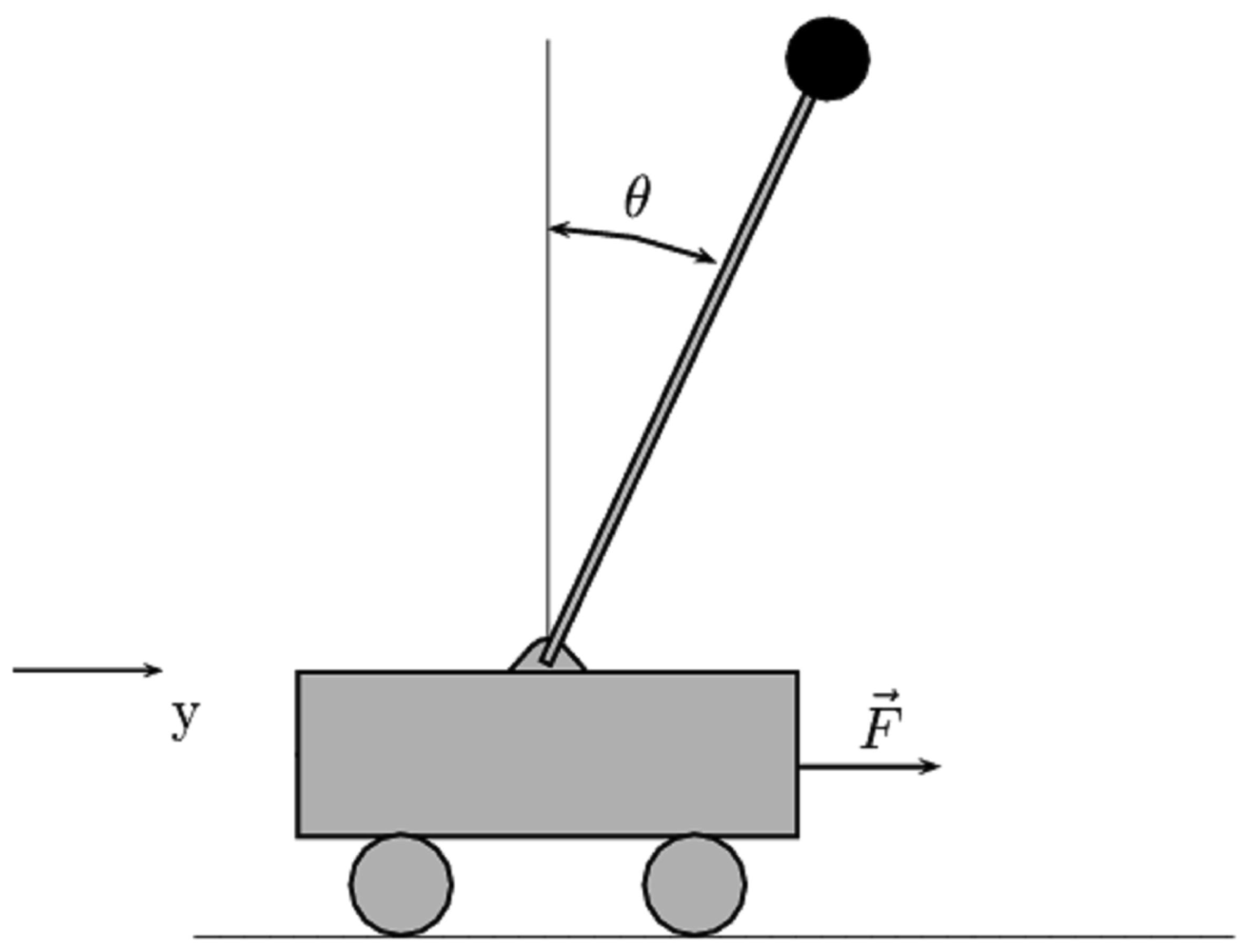
The cart-pole system, as sketched in Figure 1, is a widely used testbed for the effectiveness of control strategies. The system is composed of a pendulum and a cart. The pendulum has its mass above its pivot point, which is mounted on a cart moving horizontally. In this part, we apply the proposed control method to the cart-pole system to test the effectiveness of our method.
5.1. The Model
The cart-pole model used in this work is the same as that in [29], which can be described as follows.
g: 9.8 m/s2, acceleration due to gravity;
mc: 1.0 kg, mass of cart;
m: 0.1 kg, mass of pole;
l: 0.5 meter, half-pole length;
μc: 0.0005, coefficient of friction of cart on track;
μp: 0.000002, coefficient of friction of pole on cart;
F: ±10 Newtons, force applied to cart center of mass.
This system has four state variables: y is the position of the cart on track, θ is the angle of the pole with respect to the vertical position, and ẏ and θ̇ are the cart velocity and angular velocity, respectively.
Define , , , , A5 = mc + m, A6(θ,θ̇) = mlθ̇ sinθ, A7(θ) = –ml cosθ. With these notations, Equation (19) can be re-written as:
By choosing
5.2. Experiment Setup and Results
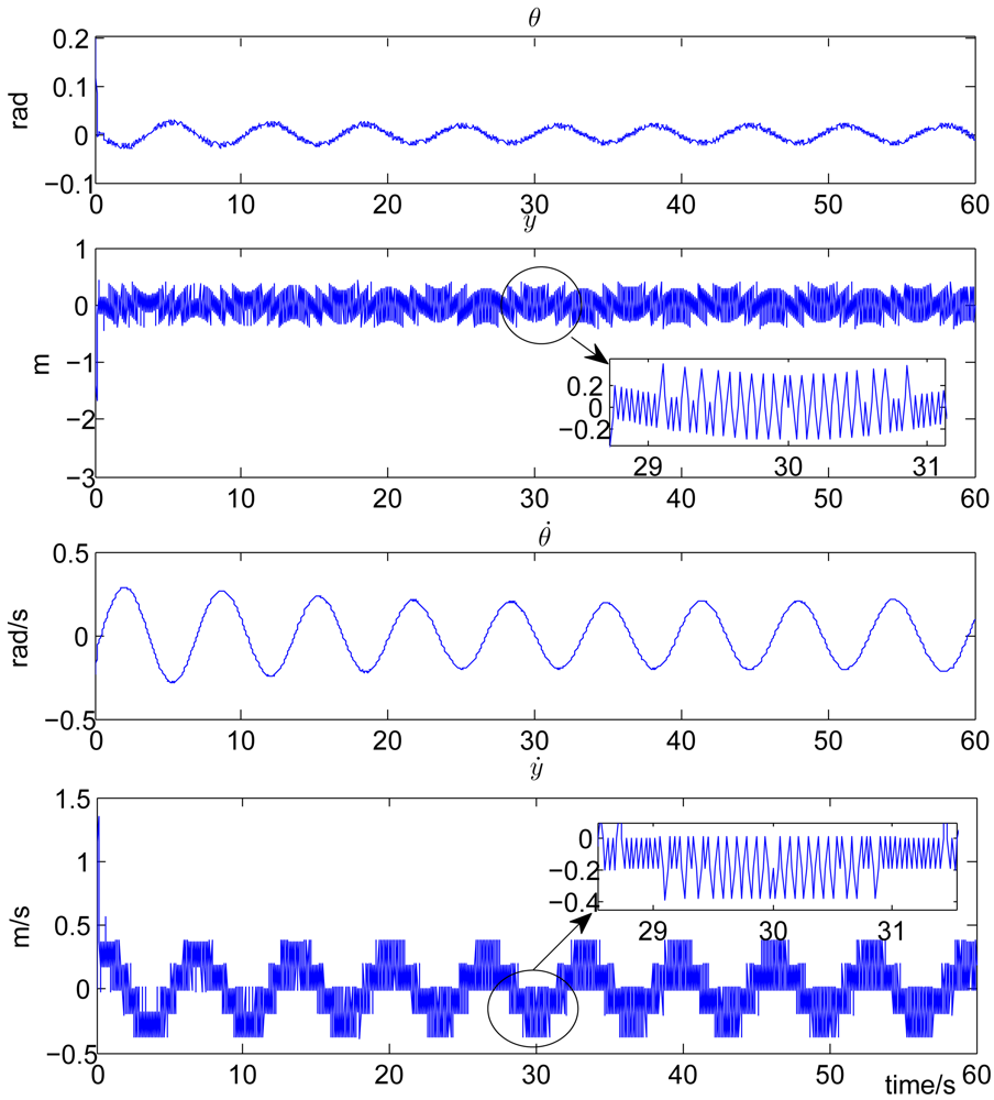
In the simulation experiment, we set the discount factor γ = 0.95, the sliding surface parameter k = 10, δ1 = 2, δ2 = 24. The feasible control action set Ω in Equation (7) is defined as Ω = {u = [u1,u2]T,u1 ∈ ℝ,u2 ∈ ℝ,u1 = u2 = ±10 Newtons}. This definition corresponds to the widely used bang-bang control in industry. To make the output of the action model within the feasible set, the output of the action network is clamped to 10 if it is greater than or equal to zero and clamped to – 10 if less than zero. The sampling period τ is set to 0.02 seconds. Both the critic model and the action model are linearly parameterized. The step size of the critic model, which is lc(n) and that of the action model, which is la(n) are both set to 0.03. Both the update of the critic model weight Wc in Equation (16) and the update of the action model weight Wa in Equation (18) last for 30 seconds. For the uncontrolled cart-pole system with F = 0 in Equation (19), the pendulum will fall down. The control objective is to stabilize the pendulum to the inverted direction (θ = 0). Time history of the state variables are plotted in Figure 2 for the system with the proposed self-learning variable structure control strategy. From this figure, it can be observed that θ is stabilized in a small vicinity around zero (with a small error of ±0.1 rads), which corresponds to the inverted direction.
6. Conclusions and Future Work
In this paper, the self-learning variable structure control is considered to solve a class of sensor-actuator systems. The control problem is formulated from the optimal control perspective and solved via iterative methods. In contrast to existing models, this method does not need pre-knowledge on the accurate mathematic model. The critic model and the the action model are introduced to make the method more practical. Simulations show that the control law obtained by the proposed method indeed achieves the control objective. Future work on this topic includes the theoretical proof of the convergence and exploration on the performance limit of the proposed strategy. Also, the control of other mechanical systems modeled by Euler-Lagrange system, such as manipulators etc., will be explored in our future work.
Acknowledgments
Shuai Li would like to share with the readers the poem by Rabindranath Tagore “The traveler has to knock at every alien door to come to his own and one has to wander through all the outer worlds to reach the innermost shrine at the end”. The authors would like to acknowledge the support by the National Natural Science Foundation of China under Grant No. 61172165 and Guangdong Science Foundation of China under Grant No. S2011010006116 and No. 10151802904000013.
References and Notes
- Isermann, R. Modeling and design methodology for mechatronic systems. IEEE/ASME Trans. Mechatr. 1996, 1, 16–28. [Google Scholar]
- van de Panne, M.; Fiume, E. Sensor-actuator networks. Proceedings of the 20th Annual Conference on Computer Graphics and Interactive Techniques (SIGGRAPH '93), Anaheim, CA, USA, 1–6 August 1993; pp. 335–342.
- Liu, B.; Chen, S.; Li, S.; Liang, Y. Intelligent control of a sensor-actuator system via kernelized least-squares policy iteration. Sensors 2012, 12, 2632–2653. [Google Scholar]
- de Silva, C. Sensors and Actuators: Control System Instrumentation; Taylor & Francis, CRC Press: Boca Raton, FL, USA, 2007. [Google Scholar]
- Beer, F.P. Vector Mechanics for Engineers: Statics and Dynamics; McGraw-Hill: New York, NY, USA, 2003. [Google Scholar]
- Lewis, F.L.; Dawson, D.M.; Abdallah, C.T. Manipulator Control Theory and Practice; Marcel Dekker: New York, NY, USA, 2004; Volume 15. [Google Scholar]
- Li, S.; Chen, S.; Liu, B.; Li, Y.; Liang, Y. Decentralized kinematic control of a class of collaborative redundant manipulators via recurrent neural networks. Neurocomputing 2012, 8, 108–121. [Google Scholar]
- Li, S.; Meng, M.Q.H.; Chen, W. SP-NN: A novel neural network approach for path planning. Proceedings of IEEE International Conference on Robotics and Biomimetics, Sanya, Hainan, China, 15–18 December 2007; pp. 1355–1360.
- Bloch, A.M. Nonholonomic Mechanics and Control; Springer-Verlag: New York, NY, USA, 2003. [Google Scholar]
- Yu, H.; Liu, Y.; Yang, T. Tracking control of a pendulum-driven cart-pole underactuated system. Proceedings of IEEE International Conference on Systems, Man and Cybernetics, Montreal, QC, Canada, 7–10 October 2007; pp. 2425–2430.
- Seifried, R. Two approaches for feedforward control and optimal design of underactuated multibody systems. Multibody Syst. Dynam. 2012, 27, 75–93. [Google Scholar]
- Isidori, A. Nonlinear Control Systems II; Springer-Verlag: New York, NY, USA, 1999. [Google Scholar]
- Primbs, J.A.; Nevistic, V.; Doyle, J.C. Nonlinear optimal control: A control lyapunov function and receding horizon perspective. Asian J. Control 2009, 1, 14–24. [Google Scholar]
- Ortega, R.; Loria, A.; Nicklasson, P.J.; Sira-Ramirez, H. Passivity-Based Control of Euler-Lagrange Systems; Springer-Verlag: New York, NY, USA, 1998. [Google Scholar]
- Azhmyakov, V. Optimal control of mechanical systems. Diff. Equat. Nonlin. Mech. 2007, 12, 3–16. [Google Scholar]
- Huo, W. Predictive variable structure control of nonholonomic chained systems. Int. J. Comput. Math. 2008, 85, 949–960. [Google Scholar]
- Dumitrascu, B.; Filipescu, A.; Minzu, V.; Filipescu, A. Backstepping control of wheeled mobile robots. Proceedings of 15th International Conference on System Theory, Control, and Computing (ICSTCC 2011), Sinaia, Romania, 14–16 October 2011; pp. 1–6.
- Hussein, I.I.; Bloch, A.M. Optimal control of underactuated nonholonomic mechanical systems. IEEE Trans. Autom. Control. 2005, 53. [Google Scholar] [CrossRef]
- Pazderski, D.; Kozowski, K.; Krysiak, B. Nonsmooth stabilizer for three link nonholonomic manipulator using polar-like coordinate representation. In Robot Motion and Control; Kozlowski, K., Ed.; Springer: Berlin/Heidelberg, Germany, 2009. [Google Scholar]
- Cuesta, F.; Ollero, A.; Arrue, B.C.; Braunstingl, R. Intelligent control of nonholonomic mobile robots with fuzzy perception. Fuzzy Sets Syst. 2003, 134, 47–64. [Google Scholar]
- Wai, R.J.; Liu, C.M. Design of dynamic petri recurrent fuzzy neural network and its application to path-tracking control of nonholonomic mobile robot. IEEE Trans. Indust. Electr. 2009, 56, 2667–2683. [Google Scholar]
- Kinjo, H.; Uezato, E.; Duong, S.C.; Yamamoto, T. Neurocontroller with a genetic algorithm for nonholonomic systems: Flying robot and four-wheel vehicle examples. Artif. Life Robot. 2009, 13, 464–469. [Google Scholar]
- Bertsekas, D.P. Dynamic Programming and Optimal Control, 3rd ed.; Athena Scientific: Nashua, NH, USA, 2005. [Google Scholar]
- Murray, J.J.; Cox, C.J.; Lendaris, G.G.; Saeks, R. Adaptive dynamic programming. IEEE Trans. Syst. Man Cyber. 2002, 32, 140–153. [Google Scholar]
- Lewis, F.L.; Vrabie, D. Reinforcement learning and adaptive dynamic programming for feedback control. IEEE Circuits Syst. Mag. 2009, 9, 32–50. [Google Scholar]
- Si, J.; Barto, A.; Powell, W.; Wunsch, D. Handbook of Learning and Approximate Dynamic Programming; John Wiley and Sons: Hoboken, NJ, USA, 2004. [Google Scholar]
- Mayne, D.Q.; Michalska, H. Receding horizon control of nonlinear systems. IEEE Trans. Autom. Control 1990, 35, 814–824. [Google Scholar]
- Bishop, C.M. Pattern Recognition and Machine Learning; Springer: New York, NY, USA, 2006. [Google Scholar]
- Si, J.; Wang, Y.T. Online learning control by association and reinforcement. IEEE Trans. Neural Netw. 2001, 12, 264–276. [Google Scholar]
© 2012 by the authors; licensee MDPI, Basel, Switzerland. This article is an open access article distributed under the terms and conditions of the Creative Commons Attribution license (http://creativecommons.org/licenses/by/3.0/.)
Share and Cite
Chen, S.; Li, S.; Liu, B.; Lou, Y.; Liang, Y. Self-Learning Variable Structure Control for a Class of Sensor-Actuator Systems. Sensors 2012, 12, 6117-6128. https://doi.org/10.3390/s120506117
Chen S, Li S, Liu B, Lou Y, Liang Y. Self-Learning Variable Structure Control for a Class of Sensor-Actuator Systems. Sensors. 2012; 12(5):6117-6128. https://doi.org/10.3390/s120506117
Chicago/Turabian StyleChen, Sanfeng, Shuai Li, Bo Liu, Yuesheng Lou, and Yongsheng Liang. 2012. "Self-Learning Variable Structure Control for a Class of Sensor-Actuator Systems" Sensors 12, no. 5: 6117-6128. https://doi.org/10.3390/s120506117
APA StyleChen, S., Li, S., Liu, B., Lou, Y., & Liang, Y. (2012). Self-Learning Variable Structure Control for a Class of Sensor-Actuator Systems. Sensors, 12(5), 6117-6128. https://doi.org/10.3390/s120506117