Article

Plant Succession in Glacier Forelands Controlled by Site Age Alone?—A Case Study at Schwarzenbergferner, Stubai Alps, Tyrol, Austria


German Alpine Club, Baden-Wuerttemberg Branch, Nature Conservation Unit, Fritz-Walter-Weg 19, 70372 Stuttgart, Germany
Diversity 2026, 18(9), 544; https://doi.org/10.3390/d18090544
Submission received: 22 July 2026 / Revised: 31 August 2026 / Accepted: 31 August 2026 / Published: 5 September 2026

Abstract

Glacier forelands are well-suited for investigating vegetation development and plant colonization dynamics in previously uninhabited areas. The areas exposed by retreating glaciers represent sites without seed banks; thus, plant colonization almost always represents a true primary succession. Vegetation dynamics relies on diaspores brought in from the surrounding. A common approach for studying long-term vegetation developments is the employment of so-called chronosequences, deriving temporal sequences from spatially different sites of various site ages. In glacier forelands, datable traces of former glacier extents are generally used for site age estimation. In 2009 and 2010, vegetation sampling for ten points in time since deglaciation was carried out in the foreland of Schwarzenbergferner, Ötz valley, Austria. The study area extends between the recent glacier terminus and the terminal moraine left by the Little Ice Age glacier during the maximum extent (around 1850). The vegetation survey is supplemented by a one-year long measurement of soil temperature (1 September 2010–31 August 2011), which allows not only for an assessment of the seasonal course of the topsoil thermal conditions across the chronosequence, but also for the determination of the snow cover duration and the length of the vegetation period. This article summarizes the vegetation development and microclimatic conditions along the chronosequence and discusses the results, considering the interplay between the time since deglaciation and elevation being a microclimatological proxy.

1. Introduction

Succession, one of the most fundamental concepts in plant community ecology [1,2], describes the development of a plant community over time. Classical ecosystems studied include sand dunes [3], old fields [4,5], volcanic ash [6], and glacial till [7,8]. A distinction is made between primary and secondary succession [9], the former occurring on newly created ground without any diaspores, the latter on disturbed ground, where pre-existing plant communities, or, at least, seedbanks to initiate succession, exist. A common approach for investigating plant succession is the employment of so-called chronosequences. It is a “space-for-time substitution” in the sense of Pickett [10], deriving a temporal sequence by spatially different sites of various site ages. Despite some shortcomings [11], chronosequences are commonly employed to investigate vegetation developments, that exceed the lifespan of an investigator. According to Walker et al. [12], succession can be successfully and sufficiently accurately explored, if plant communities are following convergent successional trajectories and chronosequences are interpreted carefully.
Key locations for the study of primary succession are in front of a retreating glacier [13]. The renowned ecologist Heinz Ellenberg [14] (p. 440) aptly states: “Nowhere can succession be studied more profitably than in the valley below the front of a large glacier”. Since the end of Little Ice Age (LIA) around 1850, the glaciers of the Alps are retreating, accelerated in recent decades. During the last one and a half to two centuries, alpine glaciers lost more than 50% of their LIA area [15,16,17,18,19], continuously enlarging the “glacier forelands”, a term introduced by Kinzl [20] for the ground between the recent glacier termini and the terminal moraines left by the LIA glaciers. Studies on vegetation development in the glacial forelands of the Alps have a long tradition. The earliest accounts date back to the 19th and early 20th century (e.g., refs. [21,22,23,24,25,26,27,28,29,30,31]). Glacier foreland studies remain highly relevant today in light of the accelerated climate warming and changes in the ice balance [16,18,19].
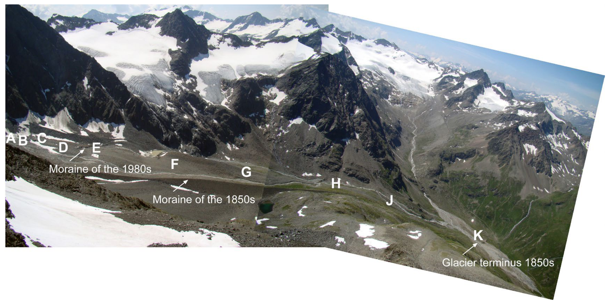
In glacier forelands of the European Alps, chronosequence studies are widespread (e.g., refs. [32,33,34,35,36,37,38,39,40,41]). The reconstruction of the site age (i.e., time since deglaciation) relies on datable traces of the former glacier extent (moraines) as well as other length change records, e.g., by historical maps, aerial photographs, or satellite imagery (e.g., refs. [38,40]). The assumption is that the increasing distance to the recent glacier terminus represents an earlier date of deglaciation in the past, and, thus, locations in different successional stages are encountered. This method is well-suitable for revealing differences in the species numbers, ground cover values, and vegetation structure, as well as species composition and diversity across study sites. However, as different areas with potentially different biotic and abiotic site factors (e.g., slope, elevation, aspect, substrate, disturbance history, seed sources in the surrounding, etc.) are investigated, it is not only the time since deglaciation that may be a relevant factor for vegetation development. In glaciated high mountain environments, the time since deglaciation often is accompanied by a change in elevation, which, in turn, goes hand in hand with a change in microclimatic conditions (changes in air and soil temperatures, duration of snow cover, and length of the growing season), factors relevant for the vegetation development observed as well. This paper presents the results of a chronosequence study in the foreland of Schwarzenbergferner (SBF—“ferner” is a Tyrolian toponym for glacier) in the Eastern European Alps (Figure 1).
The main objectives of the paper are as follows:
  • How is the plant composition, vegetation structure and phytodiversity along the chronosequence covering roughly one and half century?
  • As there is a pronounced vertical distance between the highest (=youngest) and lowest (=oldest) sites, what is the elevational gradient of the bioclimatic factors?
  • Can vegetation development in the glacier foreland of SBF accurately be explained by the time since deglaciation, as it is done in many glacier forelands?

2. Materials and Methods

2.1. Study Area

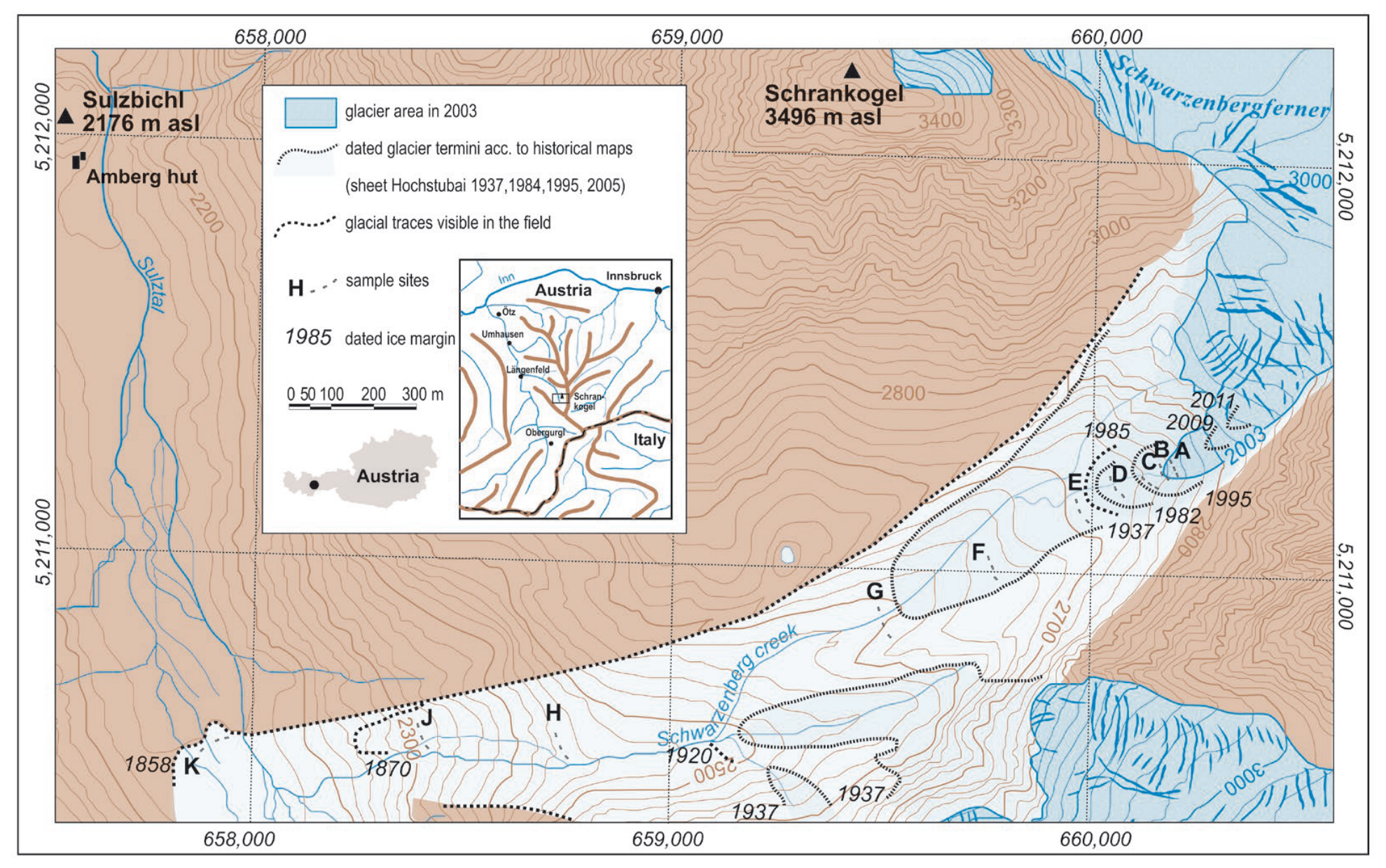
SBF descends from the southeast side of Schrankogel (3497 m asl, UTM 32T E: 659,431, N: 5,212,216) towards the Sulz valley, a tributary on the East of the Ötz valley in the Stubai Alps of Tyrol (Austria). The terminus at the time of vegetation sampling have been on the southwest-facing slope at approximately 2830 m asl (see Figure 2).
From here, the glacier foreland, deglaciated since LIA around 1858, extends for more than two kilometers and over 600 vertical meters to a distinctive terminal moraine, which marks the LIA maximum extent of the SBF, presumably united with the glacier tongue of Sulztalferner at that time. Geologically, Schrankogel belongs to the East Alpine crystalline complex (“Ötztal-Stubai Complex”) [42]. It is considered part of the Upper East Alpine nappe system, the highest tectonic unit of the Eastern Alps. Crystalline paragneisses and mica schists predominate.
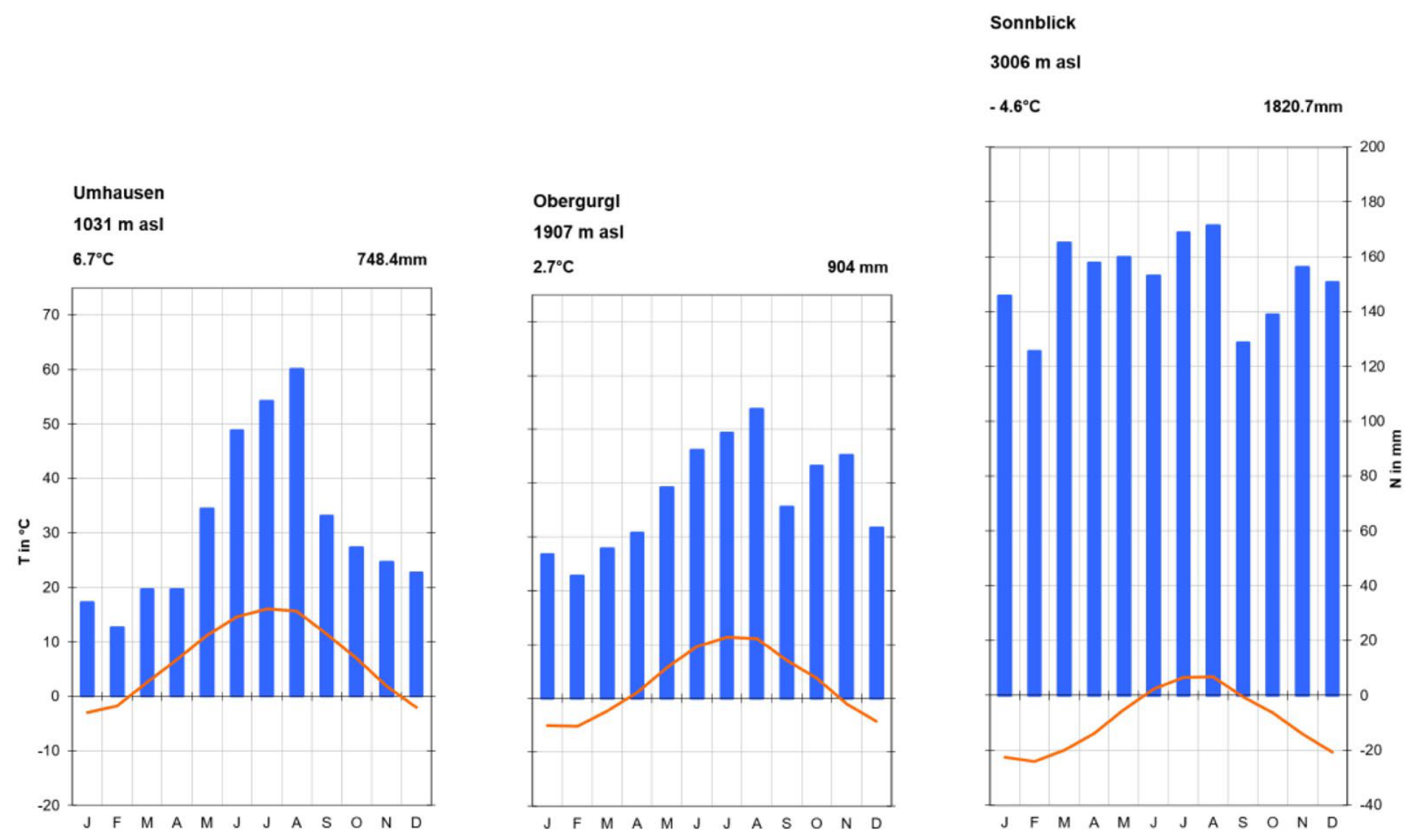
From a macroclimatic perspective, the Alps are transitional from the temperate Central European climate in the North to a Mediterranean type climate in the South. As a prominent topographic barrier, the Alps cause orographic precipitation on the outer slopes, both in the North and in the South. The more continental central Alps experience significantly lower precipitation and higher solar radiation at all elevations. The Inn Valley and the lower sections of its tributaries are typical inner-Alpine dry valleys, showcased by the climate diagram of Umhausen (1031 m asl) in the lower Ötz valley (Figure 3, ref. [43]). The station Obergurgl (1907 m asl) in the upper Ötz valley is characteristic of the climatic conditions at middle elevations, virtually at the lower end of the SBF chronosequence (Figure 3, ref. [43]). The station Sonnblick (3106 m asl) in the Hohe Tauern, located approximately 140 km east of the Ötz valley, represents the climatic conditions near the upper end of the chronosequence, i.e., in the recently deglaciated glacier foreland. The average annual precipitation at Hoher Sonnblick is 1800 mm. The average annual temperature on the Sonnblick is −4.6 °C, with positive mean temperatures occurring only for a few weeks in summer (Figure 3, ref. [43]). A large proportion of the precipitation at higher elevations falls as snow, resulting in thick and long-lasting snowpacks. Since the end of the LIA, a warming trend has been observed in the Eastern Alps. At 2 °C, the Alpine region is experiencing twice the warming of the global average due to albedo-driven feedback mechanisms [44,45,46,47]. Particularly in the summer months, a decline in snowfall at high elevations in the Alps has been observed over the last few decades.
The vertical climate gradient (temperature, precipitation snow cover, etc.) create a pronounced vertical differentiation of vegetation, soils, and morphodynamics. Concerning vegetation, the study area is mostly within the alpine (dwarf shrubs and meadows) and subnival zone (scree slopes with cushion plants and pioneer species with low ground cover). The lowest sample sites close to the LIA terminal moraine are already located in the potential subalpine coniferous forest zone. The current lack of trees at this elevation is likely due to past anthropogenic influences, as is the case elsewhere in the Alps. Permafrost is also widespread, as evidenced by numerous rock glaciers in the upper Sulz Valley (see also [42] for the upper Ötz valley).

2.2. Data Sampling and Analyses

Sampling design in general follows Fickert [48]. Vegetation sampling was performed along a chronosequence, extending from the recent glacier terminus down to the LIA terminal moraines (Table 1). The chronosequence measures 2.1 km in length with a vertical distance of roughly 600 m between highest and lowest sample sites. In total, 10 different locations (sites A to J) were sampled, deglaciated at different points in time (A: 4 yrs.; B: 5 yrs.; C: 15 yrs.; D: 20 yrs.; E: 40 yrs.; F: 60 yrs.; G: 80 yrs.; H: 110 yrs.; J: 130 yrs.; and K: 155 yrs) (I as site nomination is missing to avoid confusion with Roman numbers I, II, and III). The date of deglaciation was assumed by a combined use of dateable geomorphological structures visible in the field (sites E, H, J, and K), historical maps showing the location of past glacier termini (sites C, D, F, and G), and the annual glacier reports (sites A and B) provided by the Austrian Alpine Club (OeAV) [49].
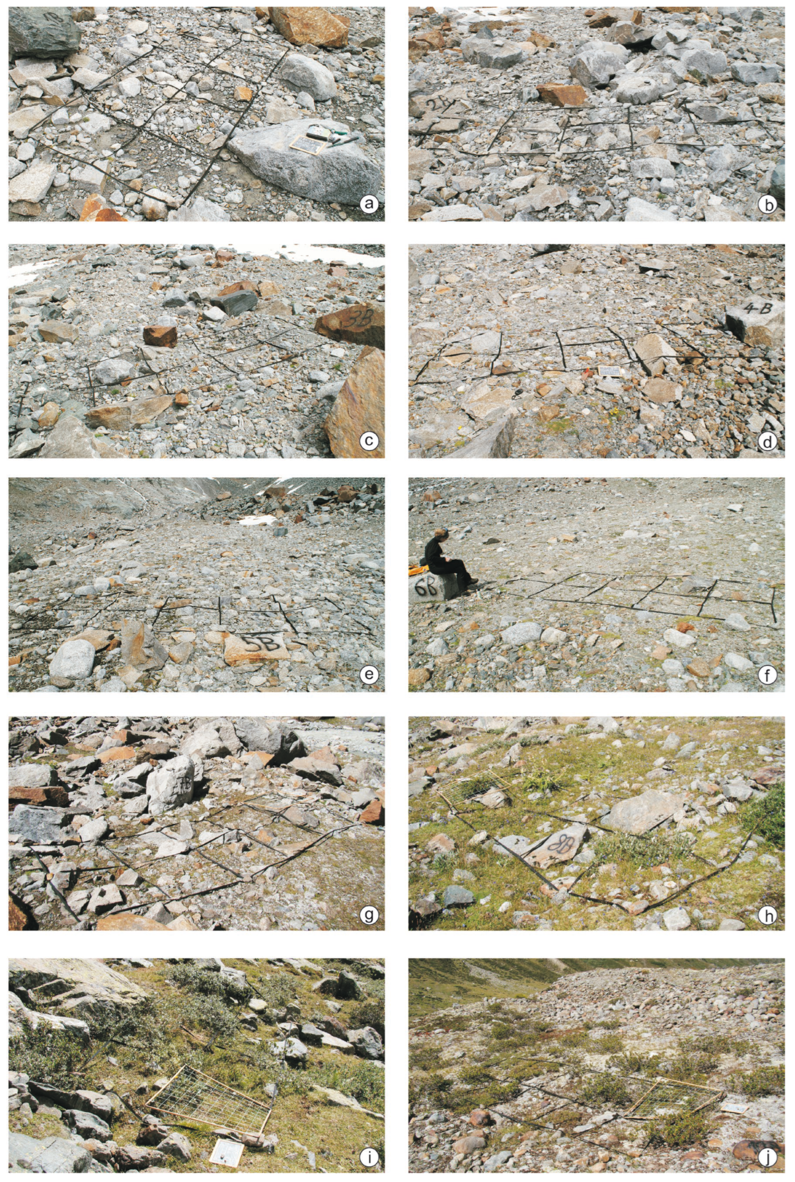
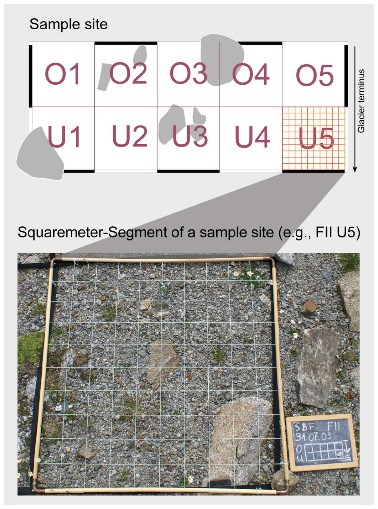
At each location A to K (see Figure 1 and Figure 2), vegetation sampling was conducted on three sample sites (I, II, and III) of 10 m2 (2 m × 5 m; Figure 4). Based on the assumption that more important changes occur during the early stages of succession compared to later ones, the time intervals between the earlier surveys are shorter. Site selection was not randomly but deliberately to avoid disturbed sites (as far as visually assessable), and to get hold of sites representing “mean” conditions—i.e., alluvial areas, wet hollows with above-average snow cover duration, or dry, wind exposed knolls were disregarded. Sites were considered typical for the respective site age. Sampling occurred square-meter-wise by visual estimation of the ground cover of each vascular plant species (taxonomy according to [50]) as well as terricolous lichen species and moss (sampled as undifferentiated species group) with the smallest unit being 0.01% ground cover (i.e., 1 cm × 1 cm on a 1 m2 subplot). The amount of coarse debris (coverage of rocks > 6 cm) was visually determined in percentage of ground cover. Raw data are subsequently converted to mean ground cover values as well as total number of species, first, per sample site (i.e., 10 m2), and, finally, for sample location (i.e., I, II, and III = 30 m2). Plots A to F were sampled in August 2009, plots G to K in August 2010. All species were assigned the corresponding life-form type (according to [51]).
To detect relationships between the species inventory and underlying site conditions, multivariate ordination methods are a common and well-suited tool. They are aimed to visualize gradients in vegetation datasets and (if available) the responsible ecological factors [52,53,54,55,56,57,58]. For this study, vegetation data were analyzed by a Correspondence Analysis (CA), i.e., an indirect, unimodal ordination procedure. That this is the appropriate response model was determined by a DCA before. As the maximum gradient calculated here exceeded the recommended threshold length of 4 standard deviations, the data exhibit a unimodal relationship between species scores and environmental variables [59].
Graphically, ordinations are depicted as two-dimensional scatter plots, with the sample sites represented as symbols. The position of each symbol in the ordination space indicates its similarity to each other. Symbols that are close together in the ordination space are similar in their species composition (if analysis is based on species inventory, as done here). Environmental variables are shown as arrows. Their length indicates the variable’s significance for the separation of the sample sites within the ordination space. The arrows point from the origin (=the mean value of a variable) to sample sites with above-average values of that variable; sample sites with below-average values are located in the opposite direction. Ordination analysis was performed by the program Canoco 4.5 [59].
The vegetation studies are complemented by one-year measurements (1 September 2010–31 August 2011) at each location of hourly soil temperatures at a depth of 10 cm, which is the main root horizon of most plants [60]. Soil temperatures have been proven to be easily measurable and biologically significant climate elements [61,62,63]. Körner [62,63] has repeatedly highlighted the decoupling of alpine plants from free atmosphere temperatures. He emphasizes that, for low-growing plants in alpine habitats with a high proportion of underground biomass, soil temperatures are probably even more important for plant physiology than air temperatures.
According to Körner [63], a soil depth of 10 cm represents a good compromise between placements that are too shallow (resulting in strong short-term fluctuations) and those that are too deep (resulting in a long response time). Soil temperature loggers of the GeoPrecision model M-Log 5 W were used, which can be read out via an infrared interface. The loggers were placed at the central out of the three sample plots at each sample location, i.e., A II to K II—see Figure 2. Since the individual sample plots hardly differ in terms of their topographical site conditions (slope, aspect, shading, microtopography, etc.), the values are considered representative for the respective elevation. With the exception of Logger B, which failed shortly before the end of the measurement period (11 July 2011), all measurement series are complete. The missing values from Logger B were supplemented using linear regression with the neighboring Logger A (R2 = 0.9814). Next to the soil temperature values, the duration of the snow cover (=isothermal conditions between day and night), temperature sums (sum of degree-hours above 5 °C), and the vegetation period (=number of days with a mean >5 °C), as well as the number of ice days (days with 24 h below 0 °C), freeze–thaw days (alternating temperatures below and above 0 °C within a day), and frost-free days (days with 24 h above 0 °C), can also be derived from the logger data. In general, caution is advised when evaluating one-year measurement series, as they may be characterized by exceptional weather conditions and, thus, deviate considerably from the average climatic conditions to which the plants at their locations are adapted. Nevertheless, even such short-term measurement series are valuable for ecological interpretation, particularly when used for the comparison of individual sites, rather than for describing average site conditions [63].

3. Results

3.1. Vegetation

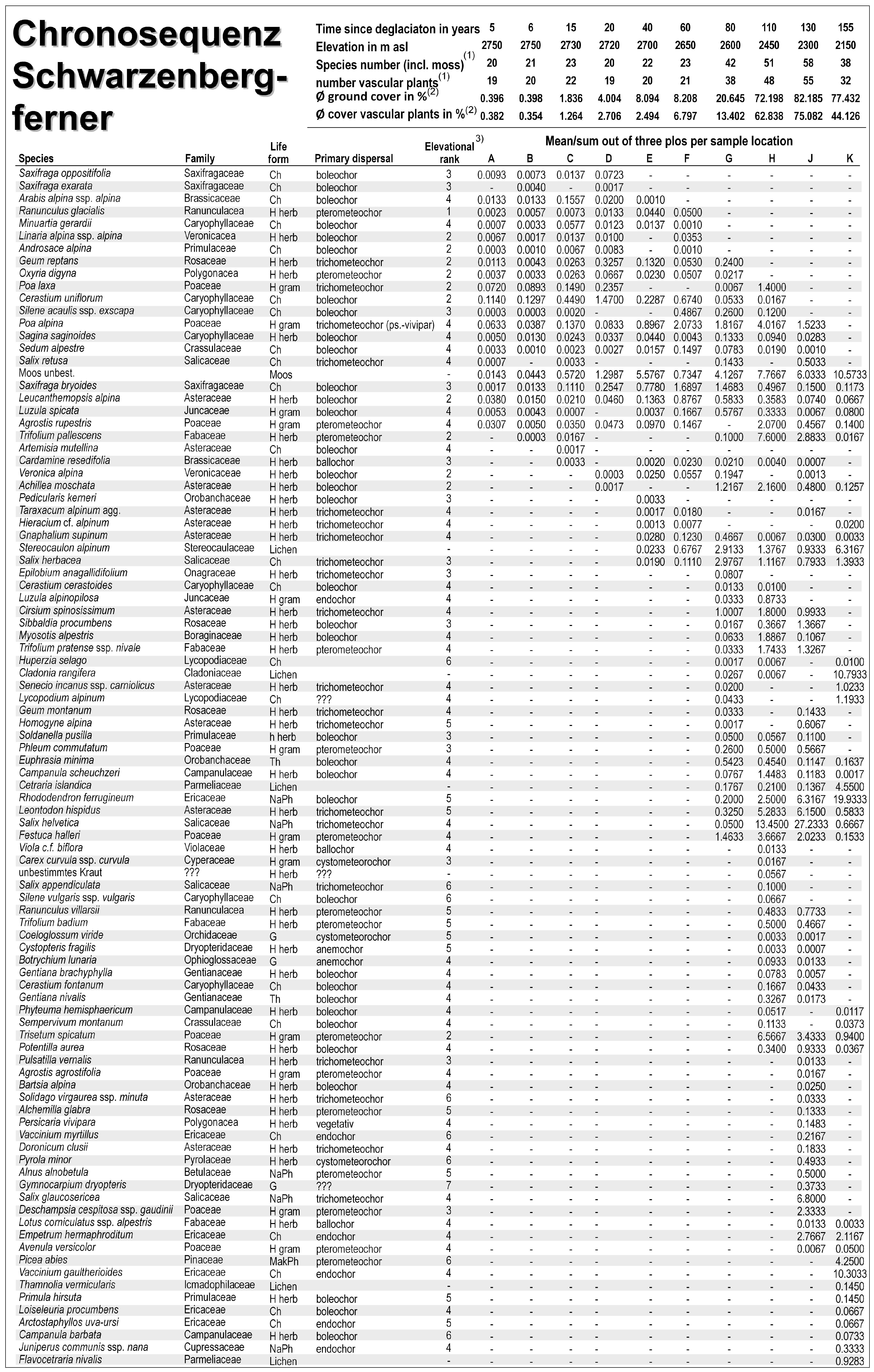
Within the 30 phytosociological samples in the glacier foreland of SBF, a total of 90 vascular plant species, 5 terricolous lichens, and moss as species group (Figure 5) were encountered. Table 2 gives key figures for the ten sample locations of the SBF chronosequence.
The A samples (Figure 6 and Figure 7), located at an elevation of 2750 m asl, are characterized by 37% coarse debris content. According to the annual glacier report of 2004 provided by the OeAV [49], it can be assumed that these areas became deglaciated in this year, i.e., five years prior to vegetation sampling. In addition to mosses, 19 different species of vascular plants have, meanwhile, been established—however, with a very low ground cover (~0.4% on average). Early colonizers include Arabis alpina, Cerastium uniflorum, Oxyria digyna, Sagina saginoides, and Saxifraga oppositifolia, as well as the grasses Poa alpina and P. laxa—common pioneer species, that also dominate early colonization in other glacier forelands of the siliceous Central Alps [35,37,39,41].
The B plots (Figure 6 and Figure 7) are located approximately 15 m away from the A plots at roughly the same elevation. The average proportion of coarse debris is higher (Table 2). On the plots, deglaciated approximately 6 years prior to sampling, 20 different vascular plant species and moss were recorded; the species composition, in general, resembles that of the A plots (see Figure 5), as does the ground cover with an average of 0.38%.
The C plots (Figure 6 and Figure 7), located approximately 75 to 80 m in front of the B plots at an elevation of 2730 m asl, were deglaciated 15 years earlier as indicated by data from the OeAV glacier measurement reports [49], and field markers from the Austrian Glacier Monitoring program close to the sample plots. The proportion of coarse debris is about 20%. A total of 22 different vascular plant species were recorded, largely identical to those in plots A and B. New species include the rare Artemisia mutellina and Cardamine resedifolia, which is also present in the later stages (Figure 5). The average ground cover is still very low with 1.3%.
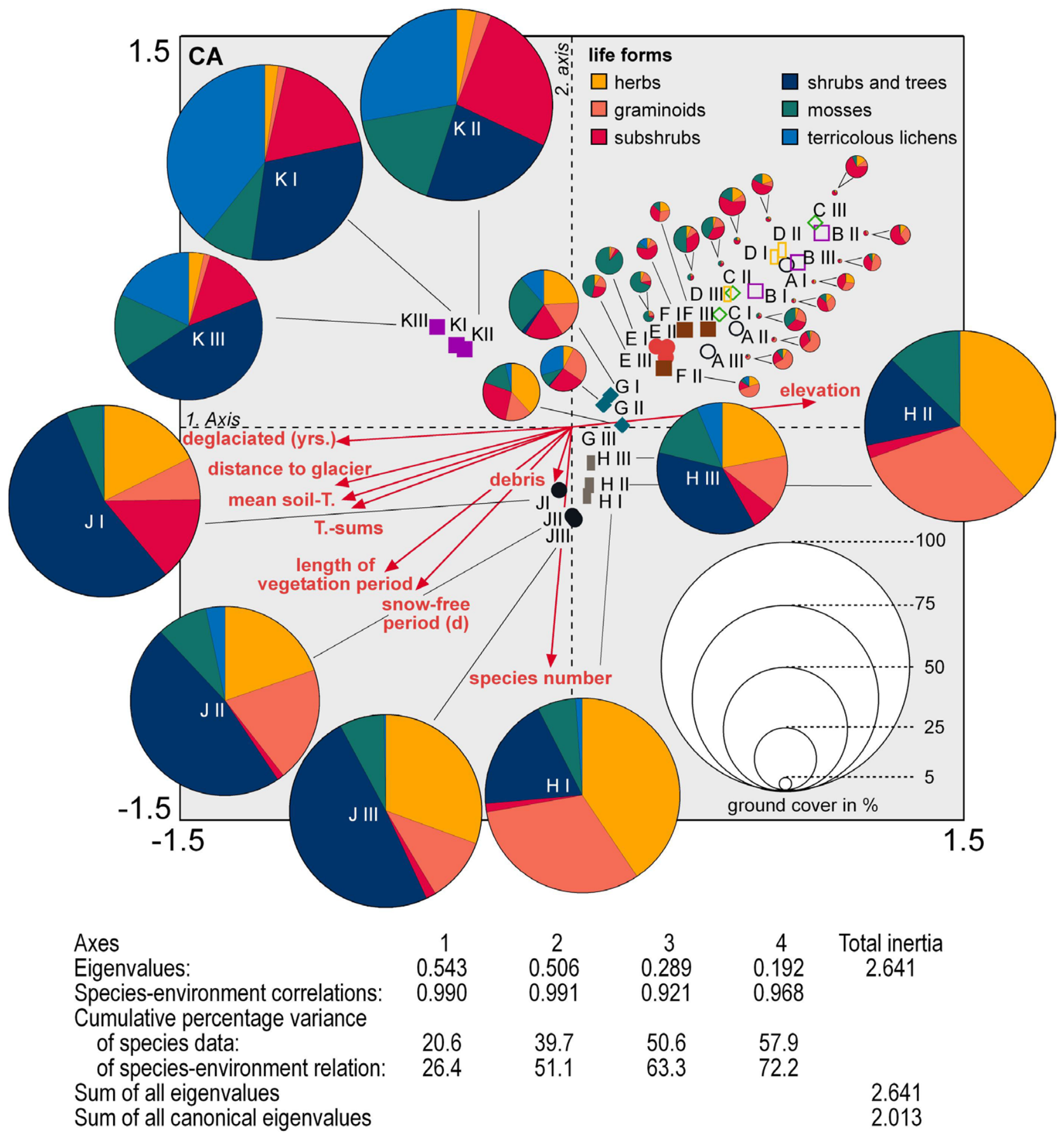
The D plots (Figure 6 and Figure 7) are located at an elevation of 2720 m asl behind a prominent rampart left by the glacial advance during the cool, wet 1970s and 1980s. Based on the OeAV glacier measurement report [49], the area likely was deglaciated a few years after the most recent phase of glacial growth, suggesting an age of approximately 20 years at the time of the survey. The number of vascular plant species is 19 and the species composition is similar to sites A to C; the average amount of coarse debris is slightly above 20%. Several of the early pioneer species are present, with Achillea moschata and Veronica alpina appearing for the first time on the D sites. With increasing distance from the recent glacier terminus and, thus, a longer period of time since deglaciation and for plant colonization, the vascular plant cover slightly increases, reaching an average of 2.7% here. With a virtually unchanged species composition (see Figure 5), all areas that are deglaciated for approximately two decades (i.e., plots A to D) can be assigned to a “pioneer stage” in plant succession. Besides the pioneers mentioned above, Leucanthemopsis alpina, Ranunculus glacialis, Saxifraga bryoides, and Geum reptans, as well as the grass Agrostis rupestre, are other common species. In the ordination plot shown in Figure 7, all sites representing the pioneer stages appear in a unique and widespread cluster, underscoring the irregular and highly random species composition during early colonization. A striking feature of this early stage is the high proportion of woody subshrubs (chamaephytes; see Figure 7).
The E plots (Figure 6 and Figure 7) are located on a flat area in front of the 1980s moraine at an elevation of 2700 m asl. The plots were deglaciated for about 40 years at the time of sampling. The average cover of coarse debris is roughly 16%. A total of 20 vascular plant species were recorded here, making up for the average ground cover of 2.5%, while the cover values can be as high as 10%+ with an above-average moss content (see plot E I). In general, the moss cover is highest on the E plots, decreasing both towards younger and older sites (Figure 7). The cryptogam cover probably declines in the later successional stages due to the increased competition for light in the progressively denser vegetation cover. The terricolous lichen Streocaulon alpinum is also represented in the E plots for the first time.
The F-plots (Figure 6 and Figure 7) are located approximately 250 m further away on another flat area at an elevation of 2650 m asl. These plots were assumed to be deglaciated for approximately 60 years. Poor in coarse rocks (7.2%), the F-plots harbor a total of 21 vascular plants species. The total ground cover of vascular plants slightly increases to an average of 6.8%. Plots E and F (40 to 60 years ice-free) represent an early successional stage in which most of the aforementioned pioneer species are still present, associated with later successional species. This early successional stage exhibits a mixture of dwarf shrubs, grasses, and herbs in varying proportions. Characteristic features include the first appearance of the ground-dwelling lichen Stereocaulon alpinum, herbs such as Gnaphalium supinum, Hieracium cf. alpinum, and the dwarf willow Salix herbacea. The replacement of the pioneer species Saxifraga oppositifolia and S. exarata indicates signs of competition. Regarding the total number of species per plot (20 and 21 vascular plants), this early successional stage does not differ much from the pioneer stage (plots A to D), but the cover values are somewhat higher (Figure 7).
Plots G (Figure 6 and Figure 7) are located approximately 300 m away from plots F at an elevation of 2600 m asl. They were deglaciated roughly for 80 years. Almost half of the sample sites are covered by coarse debris. With a total of 38 species of vascular plants and 2 new terricolous lichens (Cladonia rangifera and Cetraria islandica), this stage is significantly more species-rich than the younger sites. While some initial colonizers disappear, including Ranunculus glacialis, Minuartia gerardii, Linaria alpina, and Androsace alpina, several new species appear, absent in the pioneer and early successional stage (see Figure 5). Among these, Cirsium spinosissimum, Euphrasia minima, and Festuca halleri are particularly noteworthy in terms of frequency and/or cover. The total ground cover now reaches 20 to 25%, with the average cover of vascular plants at 13.4%. Terricolous lichens and mosses locally cover larger areas, but, in general, the proportions of the life-forms are rather balanced (Figure 7). This later successional stage can be classified as an initial grassland rich in herbs and grasses, although it has not yet developed into its typical form [39].
The H plots (Figure 6 and Figure 7) are located approximately 700 m away from the G plots at an elevation of 2450 m asl, and were estimated to be about 110 years old. The coverage of coarse debris is approximately 35%. With 48 different vascular plants, as well as mosses and two terricolous lichens, the plots are species-rich, and the total ground cover increases sharply to values exceeding 60%. Important species here include the herbs Campanula scheuchzeri, Leontodon hispidus, and various clover species (Trifolium pallescens, T. pratense ssp. nivale, and T. badium), which may play an important role in the nitrogen enrichment of the poorly developed soils [64]. Among the grasses, Poa alpina, Festuca halleri, and, especially, Trisetum spicatum stand out with a higher ground cover. Shrubs, particularly Salix helvetica and Rhododendron ferrugineum, become more important than in earlier stages, making these areas representative for a shrub-rich phase of the later successional stages.
The J plots (Figure 6 and Figure 7) are located at an elevation of approximately 2300 m on a steep slope and are assumed to be deglaciated for about 130 years. The ground cover of coarse debris is roughly 30%. With 55 different vascular plants, these are the most species-rich plots along the chronosequence. The total ground cover of vascular plants reaches 75%; about half is represented by phanerophytes (Figure 7). In addition to the shrub species mentioned above, Salix glaucosericea and Empetrum hermaphroditum are also present. These are well-developed shrub communities, characteristic of the late successional stages.
The K plots (Figure 6 and Figure 7) are located at an elevation of 2150 m just behind the LIA terminal moraine. For these plots, a site age of approximately 150 years can be assumed. The plots are flat with an average cover of coarse debris of 25%. With 32 different vascular plant species, the species richness is considerably lower than that of the J plots, and, also, the ground cover of vascular plants decreases in favor of the terricolous lichens. They are well-represented here with five different species and high cover (Ø 22.7%). Mosses reach mean ground cover values of 10.5% (Figure 7). Grasses and herbs are almost entirely absent, and hardly any of the early colonizers is left (see Figure 5). Instead, several subalpine elements are present, including the first small Picea abies individuals and Arctostaphyllos uva-ursi. Due to their unique species composition, in Figure 7, the K plots are clearly distinct from the other samples. The decreasing species numbers and ground cover values are likely due to specific microclimatic site conditions, as the valley location favors both the formation of cold air settling and a longer persistence of the snowpack due to the steep terrain and low angle of the winter sun.

3.2. Microclimate

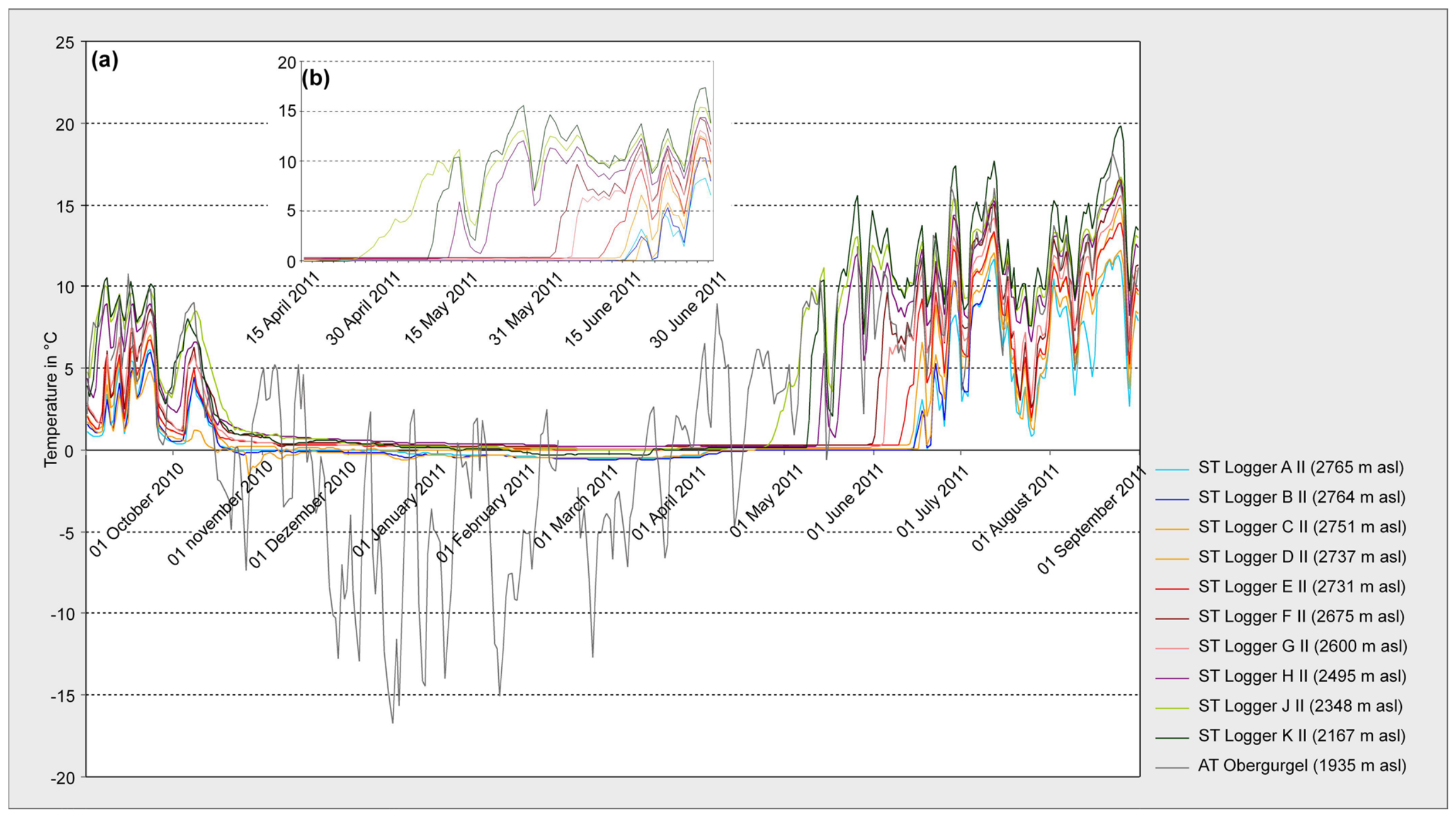
To assess the microclimatic differences between sample sites concerning factors such as soil temperature, snow cover duration (indicated by isothermal conditions between day and night), length of vegetation period (daily mean > 5°C), and temperature sums, as well as the number of ice days (ID), freeze–thaw days (FTD), and frost-free days (FFD), the soil temperature measurements are used. Figure 8 shows the annual course of the ten temperature loggers installed in the foreland of the SBF (from [60]).
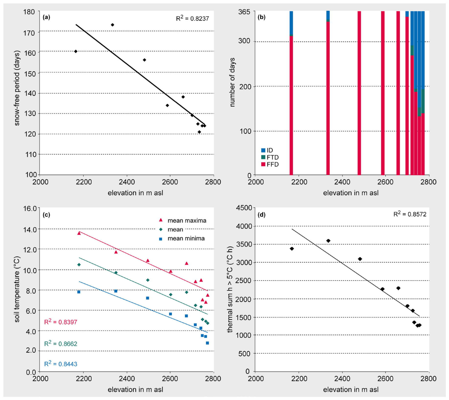
There is a pronounced vertical microclimatic gradient, finding its expression in the soil temperatures, snow cover duration, temperature sums, as well as the freeze–thaw conditions (Figure 9). The onset of winter snow is synchronous, while the date of snowmelt in spring and early summer is gradual at the individual sites (Figure 8). Between the earliest and latest day of snow cover removal (logger J II and logger C II, respectively), indicated by the restart of diurnal temperature fluctuations, is a period of time of almost eight weeks (53 days). As expected, snow melt at lower elevations is earlier than at higher elevations; however, due to topographical conditions, the lowest logger is not the earliest to become snow-free and the highest is not the latest. Particularly at logger location K II, the low-angled winter sun and the formation of cold air settling appears to favor a longer persistence of the snowpack. The proximity to the glacier terminus of the highest sites, and the possibility of dead ice in the subsurface and cool katabatic glacier winds create “supercooled” conditions close to the glacier (i.e., A, B, and C, Figure 9c). Moisture-saturated soils after snowmelt may intensify this effect, as energy is required for evaporation, energy which is therefore unavailable for warming the soil.
Finally, an upward temperature gradient is also evident for temperature sums (Figure 9d). Especially in climatically extreme alpine locations, warmth is crucial for plant life processes. According to Körner [63], 5 °C represents a critical thermal threshold for plant activity. Therefore, the heat sums, i.e., the degree-hours above this threshold, are an important indicator of the period of favorable conditions for plant growth in alpine regions—the higher the heat sums, the better. Here, too, the areas in the immediate glacier foreland and location K in the valley are cooler than expected by elevation and negatively diverge from the trend. The values range from over 1000 °h in the immediate glacier foreland to over 3000 °h in the lower elevations of the SBF glacier foreland.

4. Discussion

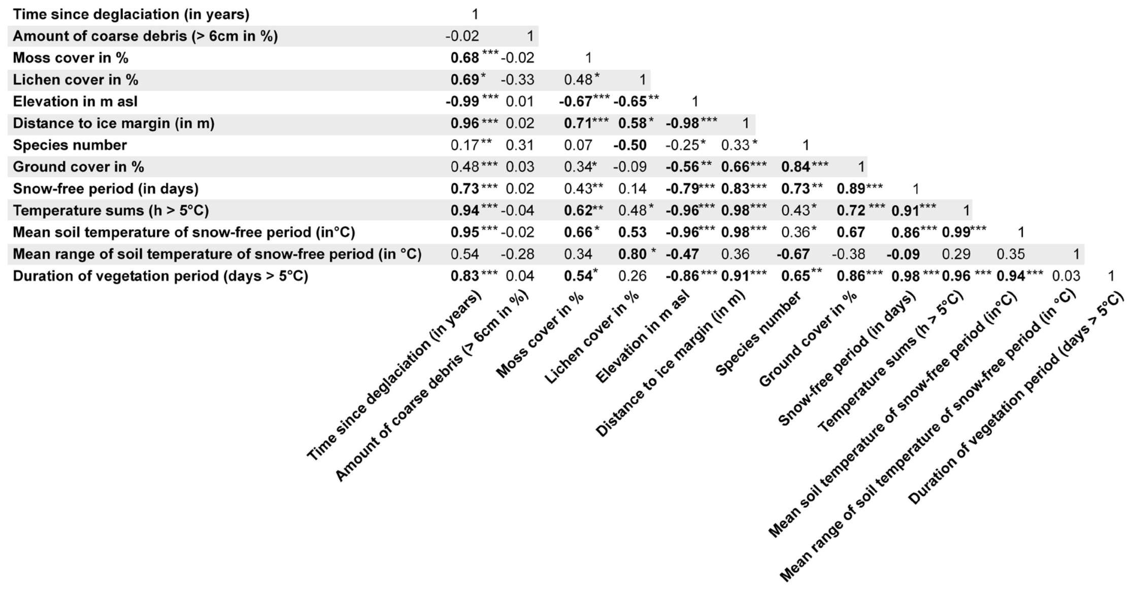
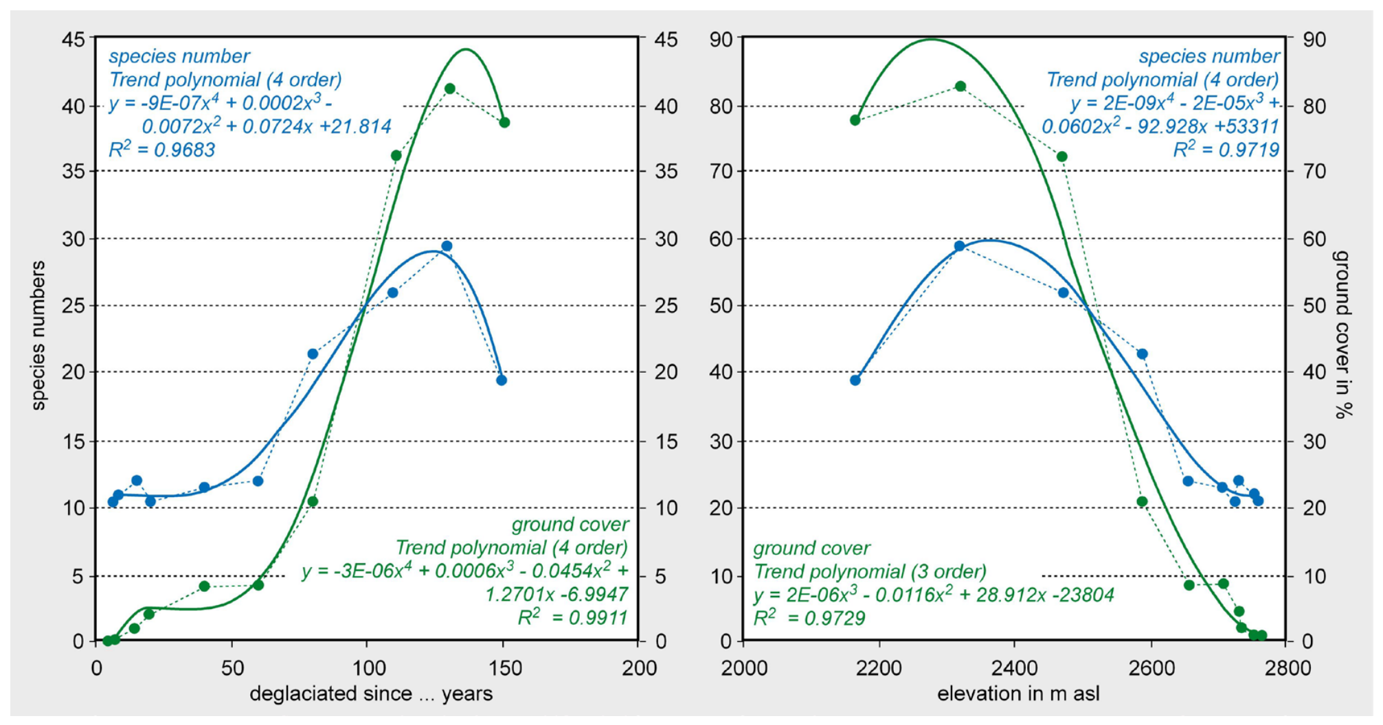
Along the SBF chronosequence, different successional stages can be identified, each expressed by a specific set of plant species and vegetation structure, as well as certain statistical parameters, such as species numbers or ground cover values. The environmental variables in the CA-ordination (Figure 7) show that the factor “time since deglaciation” is highly correlated to the first ordination axis and has a high explanatory power for the separation of the vegetation samples within the ordination space. However, next to varying dates of becoming deglaciated, the chronosequence is characterized by a pronounced vertical distance of 600 m as well, which is—as shown above—associated with an elevational gradient in bioclimatic parameters. The comparable lengths of the arrows representing site age and bioclimatic variables in Figure 7 indicate that the latter are equally important for the arrangement of the sample sites within the ordination space. The almost opposite orientation to the variable “elevation” implies a high correlation between the site age and the complex variable elevation and its associated bioclimatic variables (see Figure 10). This is hardly surprising, since, in a topographically highly structured region like the Alps, glacier forelands are commonly associated with an elevational gradient. The primary succession in glacier forelands is generally characterized by an increase in species richness and ground cover with site age. At SBF, as well, a strong non-linear relationship of increasing species numbers and ground cover values with site age exists (see Figure 11).
However, if species richness and coverage are related to the complex variable “elevation” used as bioclimatic proxy, the explanatory power is virtually identical (see Figure 11). Therefore, the site age is a good predictor for the successional development of vegetation in glacier forelands, if one individual chronosequence is considered. If two or more chronosequences are compared (e.g., refs. [37,39]), other factors (e.g., at SBF, bioclimatic ones summarized under “elevation”) come into play. This illustrates the site-specific differences in the vegetation development of glacier forelands that cannot be explained by the time since deglaciation alone [8,13,37,39,65]. From case-to-case factors such as grain size, moisture, snow cover duration, inclination, solar radiation (shade vs. sun), thermal conditions, geology (siliceous vs. calcareous) geomorphological processes, and frequencies and/or magnitudes of disturbances, as well as biotic drivers and interactions such as competition, facilitation, and allelopathy, affect and modify the successional trajectory, which might be responsible for patterns observed [13,33,39,41,66,67]. In addition, the position with regard to the treeline has been proven to be crucial for successional patterns [37,39]. Proglacial areas of large glaciers extending close to or even below the treeline ecotone are colonized more rapidly and with a higher diversity—due to a richer seed pool and generally more favorable growing conditions [27,36]—than those of smaller glaciers terminating in the species-poor upper alpine or subnival zones [14].
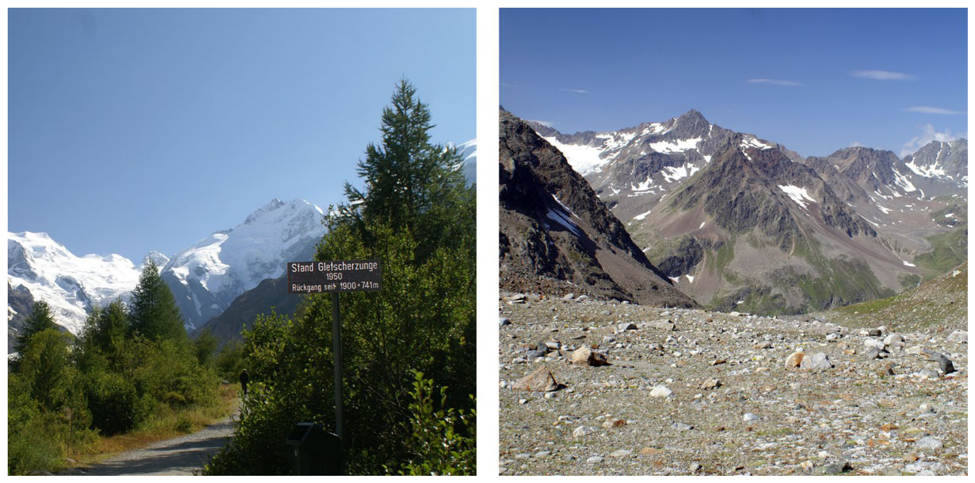
Figure 12 visualizes those site-specific differences in vegetation development by contrasting photographs of two different glacier foreland sites of roughly the same age: Morteratsch Glacier in the Engadin (Switzerland), Latitude: 46°24′20.39″ Longitude: N 9°55′32.39″ E, located just below 2000 m asl in the treeline ecotone, and SBF at 2650 m asl. While the 60-year-old site at Morteratsch harbors tall larches (Larix decidua) and alders (Alnus viridis), the higher site on SBF of the same age has not yet moved beyond a sparsely vegetated, early successional stage.
Next to the variables “time since deglaciation” and “elevation”, other factors might locally be significant for vegetation development in glacier forelands:
  • Grazing, which promotes the zoochorous dispersal of species and can lead to the selection of certain species (e.g., ref. [37]);
  • High-mountain-specific morphodynamics with its numerous disturbances, which can repeatedly throwback succession to earlier stages (e.g., refs. [67,68]);
  • Grain size composition and resulting differences in the water balance of sites (e.g., ref. [36]);
  • Differences in exposure, causing different species compositions at different sites (e.g., shady vs. sunny slopes), even though the areas are of the same age (e.g., ref. [33]);
  • Characteristics of and distance to potential seed sources, from which primary succession originates (e.g., ref. [69]).
Individual chronosequences are appropriate to identify trajectories of primary succession of plants in glacier foreland (i.e., changes in species richness, ground cover, plant functional traits, and community structure) as a function of site age and local environmental conditions. However, shifts in the species composition and general patterns in species assemblages other than the existence of various successional stages with time since deglaciation are hard to deduce, as many different factors next to site age control succession in glacier forelands.

5. Conclusions

Chronosequences allow us to study vegetation succession over periods of time much longer than a researcher’s life span. They are appropriate when there is evidence that differently aged sites are following the same trajectory [12]. In addition, they are more reliably used for developments truly related to site age (e.g., species richness, plant cover, and vegetation structure) than for those related to something else (e.g., species composition). Chronosequences can provide insights into general successional patterns as well as differences in the species composition and vegetation structure at sites with varying site ages. However, a critical evaluation of the temporal vegetation development must take into account whether factors other than site age become equally or even more important. Old field succession, in this respect, provides a rather clear picture of the temporal development on abandoned fields. Characterized by rather uniform site conditions, early successional stages on both dry and mesic fields developed at first from open annual to perennial herbal vegetation. Dry fields persist for decades in a perennial grass stage with scattered shrubs and trees, while the mesic sites develop into woodlands after two to three decades. Those general chronosequence results could be replicated by semi-permanent plots, proving that site age is indeed the responsible factor for succession on old fields [5,12].
However, glacier forelands are far more complex than abandoned fields. Vegetation dynamics and plant succession here is influenced by substrate conditions (both physical and chemical), geomorphological disturbance, hydrology, microclimate, microtopography and snow cover, seed sources, and dispersal pathways of available species, in addition to terrain age [8,33,35,39,68,70]. Therefore, in glacier forelands, chronosequences have both their values and their limitations. They allow us to identify the successional trajectory of an individual proglacial area, but, for the deduction of broad successional patterns, judiciousness should be applied, especially if environmental heterogeneity is great.
The majority of glacier foreland successions studies find that terrain age is the principal factor explaining the present-day species composition. During recent years, however, local environmental variables are increasingly being taken into account, to explain the species composition and modified local successional trajectories (e.g., ref. [71]).
As the terrain age increases and the microclimate generally becomes more favorable, it is often difficult to say whether a plant community is driven by time since deglaciation or by local environmental conditions. Microclimatic gradients and glacier retreat point in the same direction, despite being independent variables unrelated to each other. To disentangle the collinearity of the responsible factors for plant succession in glacier forelands and to confirm the considerations made here are among the challenges of future glacier foreland studies.

Funding

This research received no external funding.

Data Availability Statement

The data used are available upon request to the author.

Acknowledgments

Field work in 2009 was assisted by Friederike Grüninger, for which gratitude is expressed. Katharina Sextl and Thomas Loher supported the study with their theses on microclimate and glacial history in the glacier foreland of SBF, respectively. The author is grateful to two anonymous reviewers for the valuable recommendations, which greatly improved the outcome.

Conflicts of Interest

The author declares no conflicts of interest.

References

  1. Walker, L.R.; Wardle, D.A. Plant succession as an integrator of contrasting ecological time scales. Trends Ecol. Evol. 2014, 29, 504–510. [Google Scholar] [CrossRef] [Scilit]
  2. Fickert, T.; Richter, M. Vegetation Changes in Space and Time—A Special Issue on Plant Succession and Vegetation Dynamics. Diversity 2025, 17, 482. [Google Scholar] [CrossRef] [Scilit]
  3. Clements, F.E. Plant Succession: An Analysis of the Development of Vegetation; Publication No. 242; Carnegie Institution of Washington: Washington, DC, USA, 1916. [Google Scholar]
  4. Egler, F.E. Vegetation science concepts I. Initial floristics composition, a factor in old-field vegetation development. Vegetatio 1954, 4, 412–417. [Google Scholar] [CrossRef] [Scilit]
  5. Řehounková, K.; Tichý, L.; Prach, K. Succession in abandoned fields: Chronosequence data verified by monitoring of semi-permanent plots. J. Veg. Sci. 2024, 35, e13303. [Google Scholar] [CrossRef] [Scilit]
  6. del Moral, R. Plant succession on pumice at Mount St. Helens, Washington. Am. Midl. Nat. 1999, 141, 101–114. [Google Scholar] [CrossRef] [Scilit]
  7. Crocker, R.L.; Major, J. Soil development in relation to vegetation and surface age at Glacier Bay, Alaska. J. Ecol. 1955, 43, 427–448. [Google Scholar] [CrossRef] [Scilit]
  8. Matthews, J.A. The Ecology of Recently Deglaciated Terrain; Cambridge Studies in Ecology: Cambridge, UK, 1992; 386p. [Google Scholar]
  9. Connell, J.H.; Slatyer, R.O. Mechanisms of Succession in Natural Communities and Their Role in Community Stability and Organization. Am. Nat. 1977, 111, 1119–1144. [Google Scholar] [CrossRef] [Scilit]
  10. Pickett, S.T.A. Space-for-time substitution as an alternative to long-term studies. In Long-Term Studies in Ecology: Approaches and Alternatives; Likens, G.E., Ed.; Springer: New York, NY, USA, 1989; pp. 110–135. [Google Scholar]
  11. Johnson, E.A.; Miyanishi, K. Testing the assumptions of chronosequences in succession. Ecol. Lett. 2008, 11, 419–431. [Google Scholar] [CrossRef] [Scilit]
  12. Walker, L.R.; Wardle, D.A.; Bardgett, R.D.; Clarkson, B.D. The use of chronosequences in studies of ecological succession and soil development. J. Ecol. 2010, 98, 725–736. [Google Scholar] [CrossRef] [Scilit]
  13. Erschbamer, B.; Caccianiga, M.S. Glacier forelands: Lessons of plant population and community development. Prog. Bot. 2017, 78, 259–284. [Google Scholar] [CrossRef] [Scilit]
  14. Ellenberg, H. Vegetation Ecology of Central Europe; Cambridge University Press: Cambridge, UK, 1988; 731p. [Google Scholar]
  15. Paul, F.; Kääb, A.; Maisch, M.; Kellenberger, T.; Haeberli, W. Rapid disintegration of Alpine glaciers observed with satellite data. Geophys. Res. Lett. 2004, 31. [Google Scholar] [CrossRef] [Scilit]
  16. Zemp, M.; Roer, I.; Kääb, A.; Hoelzle, M.; Paul, F.; Haeberli, W. Global Glacier Changes: Facts and Figures; WGMS: Zurich, Switzerland; UNEP: Geneva, Switzerland, 2008; 88p, Available online: https://www.unep.org/resources/report/global-glacier-changes-facts-and-figures (accessed on 20 July 2026).
  17. Zemp, M.; Frey, H.; Gärtner-Roer, I.; Nussbaumer, S.U.; Hoelzle, M.; Paul, F.; Haeberli, W.; Denzinger, F.; Ahlstrøm, A.P.; Anderson, B.; et al. Historically unprecedented global glacier decline in the early 21st century. J. Glaciol. 2015, 61, 745–761. [Google Scholar] [CrossRef] [Scilit]
  18. Hock, R.; Rasul, G.; Adler, C.; Cáceres, B.; Gruber, S.; Hirabayashi, Y.; Jackson, M.; Kääb, A.; Kang, S.; Kutuzov, S.; et al. High Mountain Areas. In IPCC Special Report on the Ocean and Cryosphere in a Changing Climate; Pörtner, H.-O., Roberts, D.C., Masson-Delmotte, V., Zhai, P., Tignor, M., Poloczanska, E., Mintenbeck, K., Alegría, A., Nicolai, M., Okem, A., et al., Eds.; Cambridge University Press: Cambridge, UK, 2019; pp. 131–202. [Google Scholar] [CrossRef] [Scilit]
  19. Dussaillant, I.; Hugonnet, R.; Huss, M.; Berthier, E.; Bannwart, J.; Paul, F.; Zemp, M. Annual mass change of the world’s glaciers from 1976 to 2024 by temporal downscaling of satellite data with in situ observations. Earth Syst. Sci. Data 2025, 17, 1977–2006. [Google Scholar] [CrossRef] [Scilit]
  20. Kinzl, H. Formenkundliche Beobachtungen im Vorfeld der Alpengletscher; 26/29 (Klebelsberg-Festschrift); Sonderdruck aus Veröffentlichung des Museum Ferdinandeum: Innsbruck, Austria, 1949; pp. 61–82. [Google Scholar]
  21. Stotter, M.; Heufler, L. Geognostische-botanische Bemerkungen auf einer Reise durch Ötztal und Schnals. Neue Z. Ferdinandeums 1840, 6, 95–137. [Google Scholar]
  22. Kerner von Marilaun, A. Das Pflanzenleben der Donauländer; Verlag der Wagner’schen Universitäts-Buchhandlung: Innsbruck, Austria, 1863. [Google Scholar]
  23. Trentinaglia-Telvenburg, J. Das Gebiet der Rosanna und Trisanna; Carl Gerold’s Sohn: Wien, Austria, 1875. [Google Scholar]
  24. Coaz, J. Erste Ansiedlung Phanerogamer Pflanzen auf von Gletschern Verlassenem Boden; Mitteilungen der Naturforschenden Gesellschaft Bern: Bern, Switzerland, 1887; pp. 3–12. [Google Scholar]
  25. Greim, G. Studien aus dem Paznaun II, Der Jamtalferner bis 1897. Gerlands Beitr. Geophys. 1906, 8, 79–112. [Google Scholar]
  26. Rübel, E. Pflanzengeographische Monographie des Berninagebietes; Engelmann: Leipzig, Germany, 1912. [Google Scholar]
  27. Von Klebelsberg, R. Das Vordringen der Hochgebirgsvegetation in den Tiroler Alpen—Eine alpin-pflanzengeographische Studie. Osterr. Bot. Z. 1913, 63, 177–186, 241–254. [Google Scholar]
  28. Friedel, H. Die Pflanzenbesiedlung im Vorfeld des Hintereisferners. Z. Für Gletscherkunde 1938, 26, 215–239. [Google Scholar]
  29. Gams, H. Die Pflanzendecke der Vendter Täler. Festschrift zum 40jährigen Bestehen des DAV, Zweig Mark Brandenburg; Bruckmann Verlag: München, Germany, 1939; pp. 56–63. [Google Scholar]
  30. Lüdi, W. Besiedlung und Vegetationsentwicklung auf den jungen Seitenmoränen des Grossen Aletschgletschers, mit einem Vergleich der Besiedlung im Vorfeld des Rhonegletschers und des Oberen Grindelwaldgletschers. In Bericht über das Geobotanische Forschungsinstitut Rübel in Zürich für das Jahr; Stiftung Geobotanisches Forschungsinstitut Rübel: Zürich, Switzerland, 1944; Volume 1945, pp. 35–112. [Google Scholar]
  31. Lüdi, W. Beobachtungen über die Besiedlung von Gletschervorfeldern in den Schweizeralpen. Flora 1958, 146, 387–407. [Google Scholar] [CrossRef] [Scilit]
  32. Caccianiga, M.; Andreis, C. Pioneer herbaceous vegetation on glacier forelands in the Italian Alps. Phytocoenologia 2004, 34, 55–89. [Google Scholar] [CrossRef] [Scilit]
  33. Raffl, C.; Mallaun, M.; Mayer, R.; Erschbamer, B. Vegetation succession pattern and diversity changes in a Glacier Valley, Central Alps, Austria. Arct. Antarct. Alp. Res. 2006, 38, 421–428. [Google Scholar] [CrossRef] [Scilit]
  34. Cannone, N.; Diolaiuti, G.; Guglielmin, M.; Smiraglia, C. Accelerating climate change impacts on alpine glacier forefield ecosystems in the European Alps. Ecol. Appl. 2008, 18, 637–648. [Google Scholar] [CrossRef] [Scilit]
  35. Erschbamer, B.; Niederfriniger Schlag, R.; Winkler, E. Colonization processes on a central alpine glacier foreland. J. Veg. Sci. 2008, 19, 855–862. [Google Scholar] [CrossRef] [Scilit]
  36. Burga, C.A.; Krüsi, B.; Egli, M.; Wernli, M.; Elsener, S.; Ziefle, M.; Fischer, T.; Mavrisa, M. Plant succession and soil development on the foreland of the Morteratsch glacier (Pontresina, Switzerland): Straight forward or chaotic? Flora 2010, 205, 561–576. [Google Scholar] [CrossRef] [Scilit]
  37. Schumann, K.; Gewolf, S.; Tackenberg, O. Factors affecting primary succession of glacier foreland vegetation in the European Alps. Alp. Bot. 2016, 126, 105–117. [Google Scholar] [CrossRef] [Scilit]
  38. Fischer, A.; Fickert, T.; Schwaizer, G.; Patzelt, G.; Groß, G. Vegetation dynamics in Alpine glacier forelands tackled from space. Nat. Sci. Rep. 2019, 9, 13918. [Google Scholar] [CrossRef] [Scilit]
  39. Fickert, T. Common Patterns and Diverging Trajectories in Primary Succession of Plants in Eastern Alpine Glacier Forelands. Diversity 2020, 12, 191. [Google Scholar] [CrossRef] [Scilit]
  40. Knoflach, B.; Ramskogler, K.; Talluto, L.; Hofmeister, F.; Haas, F.; Heckmann, T.; Pfeiffer, M.; Piermattei, L.; Ressl, C.; Wimmer, M.H.; et al. Modelling of Vegetation Dynamics from Satellite Time Series to Determine Proglacial Primary Succession in the Course of Global Warming—A Case Study in the Upper Martell Valley (Eastern Italian Alps). Remote Sens. 2021, 13, 4450. [Google Scholar] [CrossRef] [Scilit]
  41. Ramskogler, K.; Knoflach, B.; Elsner, B.; Erschbamer, B.; Haas, F.; Heckmann, T.; Hofmeister, F.; Piermattei, L.; Ressl, C.; Trautmann, S.; et al. Primary succession and its driving variables—A sphere-spanning approach applied in proglacial areas in the upper Martell Valley (Eastern Italian Alps). Biogeosciences 2023, 20, 2010–2030. [Google Scholar] [CrossRef] [Scilit]
  42. Krainer, K. Geologie und Geomorphologie von Obergurgl und Umgebung. In Glaziale und Periglaziale Lebensräume im Raum Obergurgl; Alpine Forschungsstelle Obergurgl Band 1; Koch, E.-M., Erschbamer, B., Eds.; Innsbruck University Press: Innsbruck, Austria, 2010; pp. 31–52. [Google Scholar]
  43. Kaufmann, D. Klimadaten Nordtirol—Aufbereitete Klimamittel von GeoSphere-Stationen (Gemeinde-Datensätze); Zenodo: Geneva, Switzerland, 2026; Available online: https://zenodo.org/ (accessed on 19 July 2026). [CrossRef]
  44. Auer, I.; Böhm, R.; Jurkovic, A.; Lipa, W.; Orlik, A.; Potzmann, R.; Schöner, W.; Ungersböck, M.; Matulla, C.; Briffa, K.; et al. HISTALP—Historical instrumental climatological surface time series of the Greater Alpine Region. Int. J. Climatol. 2007, 27, 17–46. [Google Scholar] [CrossRef] [Scilit]
  45. Gobiet, A.; Kotlarski, S.; Beniston, M.; Heinrich, G.; Rajczak, J. 21st century climate change in the European Alps—A review. Sci. Total Environ. 2014, 49, 1138–1151. [Google Scholar] [CrossRef] [Scilit]
  46. Kotlarski, S.; Gobiet, A.; Morin, S.; Olefs, M.; Rajczak, J.; Samacoïts, R. 21st Century alpine climate change. Clim. Dyn. 2023, 60, 65–86. [Google Scholar] [CrossRef] [Scilit]
  47. Fuchs, S.; Schöner, W.; Steiger, R. The Austrian Alps as multi-dimensional focal area. In Second Austrian Assessment Report on Climate Change (AAR2) of the Austrian Panel on Climate Change (APCC); Huppmann, D., Keiler, M., Riahi, K., Rieder, H., Eds.; Austrian Academy of Sciences Press: Vienna, Austria, 2025; Available online: https://aar2.ccca.ac.at/chapters/7 (accessed on 14 July 2026). [CrossRef] [Scilit]
  48. Fickert, T. Glacier forelands—Unique field laboratories for the study of primary succession of plants. In Glaciers Evolution in a Changing World; Godone, D., Ed.; InTech Open: London, UK, 2017; pp. 125–146. [Google Scholar]
  49. OeAV: Archiv der Gletscherberichte. Available online: https://www.alpenverein.at/portal/museum-archiv/gletschermessdienst/archiv-gletscherberichte/archiv-gletscherberichte.php (accessed on 20 July 2026).
  50. Fischer, M.A.; Adler, W.; Oswald, K. Exkursionsflora für Österreich, Liechtenstein und Südtirol; Land Oberösterreich, Biologiezentrum der OÖ Landesmuseen: Linz, Austria, 2005; 1392p. [Google Scholar]
  51. Landolt, E.; Bäumler, B.; Erhardt, A.; Hegg, O.; Klötzli, F.A.; Lämmler, W.; Nobis, M.; Rudmann-Maurer, K.; Schweingruber, F.H.; Theurillat, J.-P.; et al. Flora Indicativa: Ökologische Zeigerwerte und Biologische Kennzeichen zur Flora der Schweiz und der Alpen; Haupt Verlag AG: Bern, Switzerland, 2010; p. 376. [Google Scholar]
  52. Whittaker, R.H. Gradient analysis of vegetation. Biol. Rev. 1967, 42, 207–264. [Google Scholar] [CrossRef] [Scilit]
  53. Orloci, L. Multivariate Analysis in Vegetation Research, 2nd ed.; Junk: The Hague, Netherlands, 1978; 462p. [Google Scholar]
  54. Gauch, H.G. Multivariate Analysis and Community Structure; Cambridge University Press: Cambridge, UK, 1982; p. 314. [Google Scholar]
  55. ter Braak, C.J.F.; Prentice, I.C. A theory of gradient analysis. Adv. Ecol. Res. 1988, 18, 271–313. [Google Scholar] [CrossRef] [Scilit]
  56. Legendre, P.; Legendre, L. Numerical Ecology, 2nd ed.; Elsevier: Amsterdam, The Netherlands, 1998; 853p. [Google Scholar]
  57. Wildi, O. Data Analysis in Vegetation Ecology; John Wiley & Sons, Ltd.: Hoboken, NJ, USA, 2010; 211p. [Google Scholar]
  58. Wildi, O. Evaluating the Predictive Power of Ordination Methods in Ecological Context. Mathematics 2018, 6, 295. [Google Scholar] [CrossRef] [Scilit]
  59. ter Braak, C.J.F.; Šmilauer, P. CANOCO Reference Manual and CanoDraw for Windows User’s Guide; Biometris: Wageningen, The Netherlands; Ceské Budejovice, Czech Republic, 2002; 499p. [Google Scholar]
  60. Sextl, K. Der Vertikale Wandel der Bodentemperaturen und der Schneedeckendauer im Oberen Sulztal (Stubaier Alpen, Tirol). Unveröff; Abschlussarbeit am Lehrstuhl für Physische Geographie; Universität Passau: Passau, Germany, 2012; 125p. [Google Scholar]
  61. Gehrig-Fasl, J.; Guisan, A.; Zimmermann, N.E. Evaluating thermal treeline indicators based on air and soil temperature using an air-to-soil temperature transfer model. Ecol. Model. 2008, 213, 345–355. [Google Scholar] [CrossRef] [Scilit]
  62. Körner, C. Alpine Plant Life; Springer: Berlin/Heidelberg, Germany; New York, NY, USA, 2003; 344p. [Google Scholar] [CrossRef] [Scilit]
  63. Körner, C. Alpine Treelines; Springer: Basel, Switzerland, 2012; 220p. [Google Scholar]
  64. Soudzilovskaia, N.A.; Aksenova, A.A.; Makarov, M.I.; Onipchenko, V.G.; Logvinenko, O.A.; ter Braak, C.J.F.; Cornelissen, J.H.C. Legumes affect alpine tundra community composition via multiple biotic interactions. Ecosphere 2012, 3, 33. [Google Scholar] [CrossRef] [Scilit]
  65. Matthews, J.; Whittaker, R. Vegetation Succession on the Storbreen Glacier Foreland, Jotunheimen, Norway. A Review. Arct. Antarct. Alp. Res. 1987, 19, 385–395. [Google Scholar] [CrossRef] [Scilit]
  66. Vetaas, O.R. Relationships between Floristic Gradients in a Primary Succession. J. Veg. Sci. 1997, 8, 665–676. [Google Scholar] [CrossRef] [Scilit]
  67. Eichel, J.; Draebing, D.; Winkler, S.; Meyer, N. Similar vegetation-geomorphic disturbance feedbacks shape unstable glacier forelands across mountain regions. Ecosphere 2023, 14, e4404. [Google Scholar] [CrossRef] [Scilit]
  68. Eichel, J. Vegetation Succession and Biogeomorphic Interactions in Glacier Forelands. In Geomorphology of Proglacial Systems. Geography of the Physical Environment; Heckmann, T., Morche, D., Eds.; Springer: Cham, Switzerland, 2019. [Google Scholar] [CrossRef] [Scilit]
  69. Erschbamer, B.; Kneringer, E.; Niederfriniger Schlag, R. Seed rain, seed bank, seedling recruitment, and survival of seedlings on a glacier foreland in the Central Alps. Flora 2001, 196, 304–312. [Google Scholar] [CrossRef] [Scilit]
  70. Fickert, T.; Grüninger, F. High-speed colonization of bare ground—Permanent plot studies on primary succession of plants in recently deglaciated glacier forelands. Land Degrad. Dev. 2018, 29, 2668–2680. [Google Scholar] [CrossRef] [Scilit]
  71. Rydgren, K.; Halvorsen, R.; Töpper, J.; Njøs, J. Glacier foreland succession and the fading effect of terrain age. J. Veg. Sci. 2014, 25, 1367–1380. [Google Scholar] [CrossRef] [Scilit]
Figure 1. “Aerial” view from Schrankogel (3497 m asl) into the glacier foreland of SBF, with the approximate location of the sample sites A to K and geomorphic surface features shown (Photograph: Thomas Fickert, August 2015).
Diversity 18 00544 g001
Figure 2. The glacier foreland of Schwarzenbergferner, Tyrol (Austria), showing ice-margin positions and glaciated area (bluish colors) since LIA and the locations of the sample plots for the vegetation studies.
Diversity 18 00544 g002
Figure 3. Climate diagrams from Umhausen (lower Ötz valley), representing the inner-Alpine dry valleys, Obergurgl (upper Ötz valley) representing the climatic conditions in the tree-line ecotone, and Sonnblick (Hohe Tauern) serving as reference for the climatic conditions at the current glacier terminus of the SBF (data mean for 1991–2020, from [43]). Orange lines represent temperatures, blue bars monthly precipitation.
Diversity 18 00544 g003
Figure 4. Vegetation sampling at Schwarzenbergferner, Tyrol, (Austria) occurred on 10 m2 plots (2 m × 5 m) with three sample sites per location A to K.
Diversity 18 00544 g004
Figure 5. Sorted species list of the chronosequence in the foreland of the SBF. Elevational ranks: 1 = subnival; 2 = alpine-subnival; 3 = alpine; 4 = subalpine-alpine; 5 = subalpine; 6 = montane-subalpine; 7 = montane. (1) sum out of three plots; (2) mean out of three plots; (3) acc. to [50].
Diversity 18 00544 g005
Figure 6. Exemplary photographs of the chronosequence at SBF glacier depicting the successional vegetation development; the middle of the three sample plots per sample location A to K are shown. Time since deglaciation: (a) AII, July 2009: 4 years; (b) BII, July 2009: 5 years; (c) CII, July 2009: 15 years; (d) DII, July 2009: 20 years; (e) EII, July 2009: 40 years; (f) FII, July 2009: 60 years; (g) GII, August 2010: 80 years; (h) HII, August 2010: 110 years; (i) JII, August 2010: 130 years; and (j) KII, August 2010: 155 years.
Diversity 18 00544 g006
Figure 7. Schwarzenbergferner, Tyrol (Ausria): CA-ordination of the vegetation plots (n = 30) along the SBF chronosequence. Environmental variables are shown as arrows. Their length indicates the variable’s significance for the separation of the sample sites within the ordination space. The pie charts show the life-form composition and total cover of the study plots; the pie charts for plots A through E are enlarged due to their low total cover for better reading.
Diversity 18 00544 g007
Figure 8. Annual courses of soil temperatures (1 September 2010 to 31 August 2011) at the ten logger sites in the glacier foreland of Schwarzenbergferner, Tyrol (Austria), and of air temperature at the station Obergurgl (Ötz valley, Tyrol, Austria) in (a); panel (b) shows a zoom for the period of the spring snow melt for all ten sites, covering a 53-day interval (modified from [60]).
Diversity 18 00544 g008
Figure 9. Schwarzenbergferner, Tyrol, Austria: Vertical gradients of selected (bio)climatic parameters at ten sites in the glacier foreland of SBF (Stubai Alps): (a) duration of the snow-free period in days; (b) number of ice days, freeze–thaw days, and frost-free days; (c) soil temperatures (mean, minimum, and maximum) during the snow-free period; and (d) temperature sums in °h > 5 °C (=sum of all degree values > 5 °C). Except for (b), all microclimatic gradients are highly significant (p < 0.01).
Diversity 18 00544 g009
Figure 10. Correlations of environmental variables recorded in front of SBF; highly correlated values exceeding +/− 0.5 are highlighted in bold, significances are shown by asterisks: * p < 0.05, ** p < 0.01, and *** p < 0.001.
Diversity 18 00544 g010
Figure 11. Trends in species richness and total vegetation cover in the glacier foreland of SBF, mean per sample location A to K for ground cover, and sum for species numbers in relation to time since deglaciation (left) and elevation (right). The explanatory power (R2) is high and virtually identical for both variables.
Diversity 18 00544 g011
Figure 12. Comparison of the glacier foreland of the Morteratsch Glacier in the Engadine (Switzerland, September 2014) located just under 2000 m asl in the treeline ecotone ((left); the signpost of the glacier path reads “glacier terminus in 1950, glacier retreat since 1900 741 m”) and the glacier foreland of SBF (right) in the Stubai Alps (Tyrol, September 2011) at 2650 m asl.
Diversity 18 00544 g012
Table 1. Key figures and environmental variables of the SBF chronosequence.
Key Figures and Environmental VariablesSpalte1
Latitude/longitude of glacier terminus at time of sampling47°02′ N; 11°00′ E
Latitude/longitude of LIA terminal moraine47°01′ N; 11°04′ E
ExposureW
Approx. temperature within glacier foreland0–3.6 °C
Approx. precipitation within glacier foreland~1000–1700 mm
GeologyMetamorphic rocks (gneiss, mica-schist)
Elevation of highest samples2780 m asl
Elevation of lowest sample2165 m asl
Horizontal extent chronosequence2100 m
Vertical extent chronosequence615 m
Number of sample locations per chronosequence10
Table 2. Schwarzenbergferner, Tyrol (Austria): key figures of the ten sample locations (each with three plots) of the SBF chronosequence; vp = vascular plants, l = lichens, m = moss (undifferentiated as group).
Sample SiteElevation
in m asl
Deglaciated Since…YearsSpecies Numbers
(vp & l & m)
Total Groundcover in %Amount of Coarse
Debris in %
A27505200.437
B27506210.447
C273015231.820
D272020204.022
E270040228.016
F265060238.27
G260080422148
H2450110517235
J2300130588232
K2150155387726
Disclaimer/Publisher’s Note: The statements, opinions and data contained in all publications are solely those of the individual author(s) and contributor(s) and not of MDPI and/or the editor(s). MDPI and/or the editor(s) disclaim responsibility for any injury to people or property resulting from any ideas, methods, instructions or products referred to in the content.