Article

Space Use in Cinereous Vultures (Aegypius monachus): The Role of Artificial Feeding

by
Dimitrios Vasilakis
1,*,
Konstantina Zografou
2,
Vasilios Liordos
3 and
Vasiliki Kati
2
1
Hellenic Republic, Didimotycho Forest Service, Adrianoupoleos 1, 68300 Didimotycho, Greece
2
Department of Biological Applications & Technology, University of Ioannina, 45110 Ioannina, Greece
3
Department of Natural Environment & Climate Resilience, Democritus University of Thrace, P.O. Box 172, 66100 Drama, Greece
*
Author to whom correspondence should be addressed.
Diversity 2026, 18(8), 466; https://doi.org/10.3390/d18080466
Submission received: 29 May 2026 / Revised: 18 July 2026 / Accepted: 27 July 2026 / Published: 1 August 2026
(This article belongs to the Special Issue Conservation and Ecology of Raptors—3rd Edition)

Abstract

The factors affecting vultures’ space use can be complex, but food availability is often considered the primary determinant. However, when vultures’ food resources become highly predictable, their role in movement ecology has been little studied. Conservation planning for endangered vulture species requires a comprehensive understanding of space use. In this study, we quantified several metrics that may affect the space use of Cinereous Vultures (Aegypius monachus), a central-place forager isolated in the southeastern Balkans, which had access to substantial artificially provided food (33 tons per year) during the study period (2004–2009). Metrics examined for putative influence on ranging behavior included season, age, sex, breeding status, and artificially provided food quantity. Home range and core area sizes were larger during the breeding season and smaller during the non-breeding season. Although age, sex, and breeding status did not affect space use, we found strong evidence that artificially provided food predictability can shape the movement ecology of Cinereous Vultures. Annual home range size, core area, and seasonal overlap of the spatial parameters did not vary greatly over the years, suggesting repeatability in the species’ ranging behavior. Highly predictable artificially provided food can modify the movement ecology of necrophagous species. Yet, providing safe food is essential to preserve this endangered vulture. We suggest that feeding programs be gradually diversified to simulate natural carrion availability by using multiple small feeding sites and supplementing them unpredictably with small amounts of food.

1. Introduction

Space use may vary with an individual’s characteristics (age, sex, breeding status) or with extrinsic environmental variation (e.g., season, food availability, weather) [1,2,3]. These differences may be especially important for long-lived, late-maturing species, such as vultures, which may exhibit age-dependent changes in foraging behavior [1,3,4,5]. A comprehensive understanding of these differences may inform targeted conservation and management actions that can safeguard vulnerable or endangered populations [5,6,7,8].
In addition to intrinsic individual characteristics and extrinsic “natural” environmental variation, human-induced variation in food resources can also shape wild animals’ movement ecology [5,9,10]. Food resources for necrophagous vultures are spatially and temporally unpredictable, so they must range widely [11,12]. For over half a century, a widely used management tool for endangered vultures has involved the deliberate, regular provision of uncontaminated food in suitable locations [13]. Such “vulture restaurants” have been widely used to mitigate fatalities caused by illegal human activities, to increase public awareness, and as an eco-tourism tool [13]. They can also reduce the risks of poisoning [14,15,16] and ingestion of contaminated food [15]. Other beneficial goals have included enhancing survival or reproductive output, thereby also contributing to the colonization or recolonization of new or abandoned breeding sites [14,17,18], or to support reintroduction programs.
Besides the many benefits, vulture restaurants can have adverse consequences, including heightened predation risk and increased potential for disease transmission [16,19]. Similarly, unintended impacts on ecological, demographic, and behavioral parameters may occur when the applied protocols do not integrate all the appropriate variables [16,20,21,22]. Moreover, recent evidence indicates that feeding stations might also affect the process of natural selection and even render individuals or populations maladapted to their natural environment [19]. The provision of large amounts of food at specific sites certainly increases the spatial and temporal availability, and thus predictability, of food. Because feeding stations are predictable food sources, vultures routinely inspect them before undertaking longer foraging trips. Food availability is also rapidly detected through social information, as vultures respond to the flight behavior of conspecifics already exploiting a carcass. This gain probably affects vultures’ natural ability to forage on unpredictable resources, but the nature of this impact on birds’ foraging behavior is little understood [5,16]. While a number of studies have investigated the consequences of surplus, site-concentrated food on the population dynamics of scavengers, relatively little is known about the effects of such practices on space use.
In this study, we evaluated variation in spatial parameters (home range and core areas) and the effect of artificial food provision on these parameters in a population of the Cinereous Vulture (Aegypius monachus), hereafter referred to as vultures, in Greece. The study area contains the sole natural Balkan breeding population of the species, and a supplementary feeding site has been provided there since 1987 [23,24]. This study provides data on the spatial patterns of 19 Cinereous Vultures of various ages. Specifically we sought to: (1) evaluate the ability of different spatial parameter estimators to provide reliable estimates for further analysis; (2) describe the size of individual and population home ranges, core areas and spatial patterns for the species; (3) evaluate the effect of sex, breeding status, season, and age class on home range size, core area size and other spatial parameters; (4) evaluate the effect of the quantity of artificially provided food at two specific and long-term operated feeding sites on vulture spatial behavior (home range and core area size and other spatial parameters) and discuss its implications for the management and conservation of this threatened species.

2. Materials and Methods

2.1. Study Area and Species

The study area was located in the Eastern Rhodopes mountains in the Balkans (Figure 1), spanning parts of Greece and Bulgaria (15,000 km2). The climate is Continental-Mediterranean, and the area features gentle topography up to 1200 m. It comprises hills covered with broad-leaved and pine woods, alternating with pastures and agricultural mosaics, and is characterized by a highly heterogeneous landscape [25,26].
The study area is sparsely populated, encompasses 22 Natura 2000 sites (15 in Greece and 7 in Bulgaria), and is home to 32 of the 38 European diurnal raptor species [27]. The unique and highly diverse assemblage of taxa (passerines, amphibians, reptiles, butterflies, grasshoppers, vascular plants) in the study area makes it a biodiversity hotspot [26,28]. The area is characterized by open agro-silvo-pastoral landscapes that have been shaped over the centuries by traditional, extensive silvicultural and pastoral practices [26,29]. It supports the target species, which nests in Dadia-Lefkimi-Soufli National Park (DLS NP) in Greece. The species averaged 24 breeding pairs during the study period (2004–2009) and maintained a relatively stable population, with an average size of 103 individuals (2004–2009: 12.7% fledglings, 11.6% juveniles, 20.3% immatures, and 55.5% adults) [23,30,31]. The Cinereous Vulture is a long-lived, obligate scavenger that is tree-nesting, non-territorial, wide-ranging, and semi-colonial, and it behaves as a central-place forager when breeding [32]. It is endangered in Greece and globally near threatened, with a declining population outside Europe [33,34]. On the Balkan Peninsula, specifically within our study area, the population is strictly resident and sedentary, with no migration beyond its year-round home range. The breeding season is extensive, spanning February through August, followed by a well-defined non-breeding season from September to January. The species exhibits complex, socially driven behaviors that vary temporally. Paired territoriality dominates the breeding phase, whereas the non-breeding season is marked by a highly social organization in which individuals frequently forage in small groups (4–6) and roost communally in forest stands or on rocks. In the absence of human intervention, the species’ normal diet in this region consists primarily of medium-to-large carcasses of wild and domestic ungulates, with a significant reliance on tortoises (Testudo spp.) in spring and summer. Conversely, the artificially provided food at the managed feeding stations during the study period consisted solely of whole carcasses or slaughtered remains of domestic livestock, primarily pigs, cattle, sheep, and goats.

2.2. Data Collection and Treatment

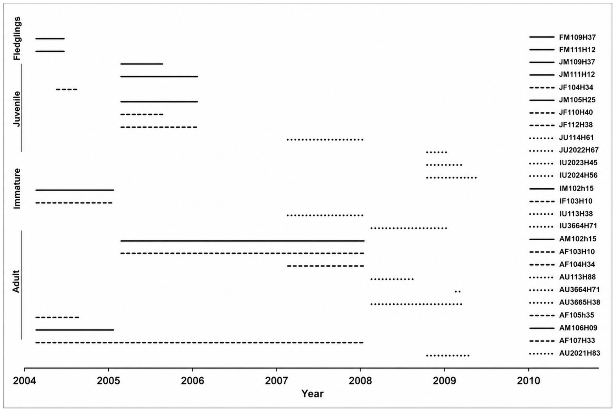
Vultures were trapped during the non-breeding season (September–January) using a walk-in cage with a sliding door. Captured vultures were aged as fledglings (1st Calendar Year; CY), juveniles (2nd CY), immatures (3rd–4th CY), or adults (≥5th CY) [35] (see Appendix A, Table A1, Figure 2). Birds were ringed, marked with patagial wing tags, and fitted with transmitters attached as backpacks via a Teflon harness [25]. Backpacks (transmitters plus harnesses) were removed as soon as tags stopped transmitting. Backpacks weighed less than 3% of each vulture’s body mass (mean mass 7944 g, SD = 657, n = 19) (Table A1), as recommended by [36]. No lesions or other physical problems were observed in birds whose tags were later removed due to non-transmission. We observed no behavioral, survival, or reproductive consequences of tagging vultures. The tagging process was conducted with specific permission from the Ministry of Environment, Energy, and Climate Change (Greece) and the Hellenic Ringing Center (Approval Code: 99110/4096 and the Approval Date: 15 October 2008).
Tagged vultures provided two datasets. The first dataset (2004–2007) comprised 12 radio-tagged individuals (radio-transmitters weighing 75 g, Model-TW3, Biotrack-Ltd., Dorset, UK), yielding 6777 locations over 316 monitoring bird-months. The second dataset consisted of 7 Global Positioning System (GPS)-tagged individuals (three GPS-Plus weighing 155 g, Vectronic Aerospace GmbH, Berlin, Germany and four Telus-Mini weighing 200 g, Televilt/TVP-Positioning, Lindesberg, Sweden), yielding 14,822 locations over 74 monitoring bird-months. More details on the datasets can be found in [25,31,37]. Both datasets were used for delineating home ranges and core areas.
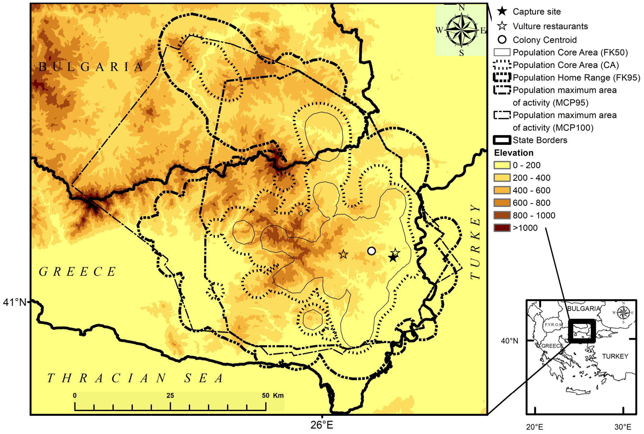
We acquired data on seasonal and annual counts of dead livestock (Table A2, WWF Dadia Project; Skartsi Th., pers. comm.), provided weekly at specific feeding sites near the breeding colony centroid (Figure 1). Carcasses were generally supplied weekly and typically consumed within the same day or the following day. Consequently, the feeding stations provided predictable but temporally pulsed food resources. The two supplementary feeding stations, one operating since 1987 and the other since 2005, were located between the breeding colony and the main foraging areas. The nests and the main communal roosting sites were located within approximately 5–7 km of the colony centroid, allowing the vultures to reach either feeding station in only a few minutes of flight.

2.3. Home Range and Core Area Estimation

We first estimated the home range for the breeding season (BS, February to August) and the non-breeding season (NBS) (Table A3). We included in the analysis only individuals with more than 50 locations per season [38]. We randomly selected only one location per tracking day from the set of locations within a buffer around nests to avoid clustering of locations around nesting sites and, consequently, underestimating the home range [38]. The buffer was defined based on a mean linear triangulation location error of 1 km [37] for the first dataset and a mean linear location error ≤ ± 9.1 m (SE = 0.15) for the second dataset, using only three-dimensional locations [39]. We included all locations (Table A3) up to the point of home range stabilization for each individual and season, determined by plotting home range size (100% Minimum Convex Polygon; MCP) against the number of locations [36]. We used the Fixed Kernel home range analysis [40,41] using a 2 × 2 km grid cell and a smoothing factor determined by least squares cross-validation to determine the home range as the 95% use-contour (FK 95), with internal range configuration in 5% steps [42]. The grid cell size was selected to reflect the spatial accuracy of the radio-tracking data (first dataset) [25]. Consequently, the second dataset was analyzed and downscaled to the same grid cell size to ensure consistency between the two datasets. The resulting Utilization Distribution (UD) offers a probabilistic representation of space use. Consequently, the estimated home range size and the density surface generated by the Fixed Kernel analysis reflect the intensity of space use, with areas of higher vulture relocation density corresponding to locations visited more frequently. We computed the 100% MCP, the 95% MCP, and the 50% fixed kernel (FK50) to enable comparison with similar studies.
The 100% MCP (MCP100) represents the maximum area of activity used, including outlier locations, whereas the 95% MCP (MCP95) indicates the maximum area used, excluding outlier locations. The FK95 and FK50 indicate the area of the home range within which the individual spends 95% and 50% of its time, respectively [36,38,42]. The home range analysis was conducted using ArcView (Version 3.2; ESRI Inc., 1994, Redlands, CA, USA) with the “Animal Movement” extension (Alaska Science Center, Anchorage, AK, USA).
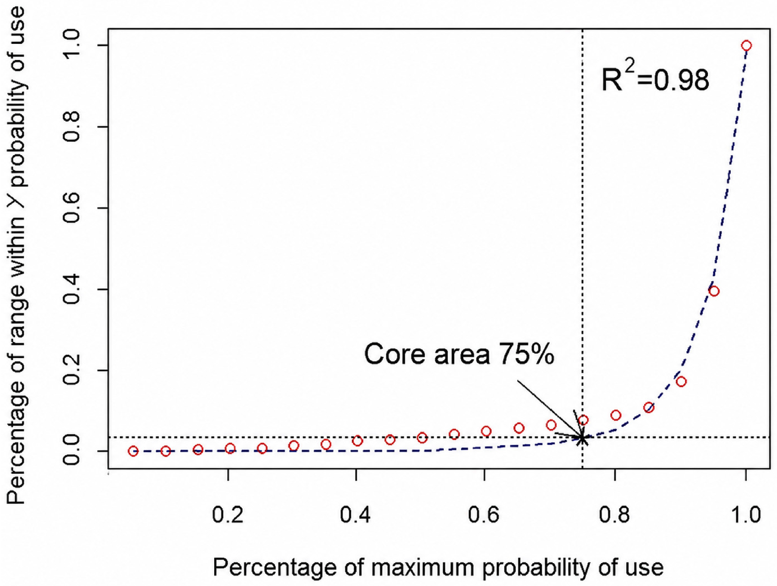
Second, we estimated the core areas (CAs) for each individual by season by integrating the fixed kernel analysis output (internal configuration, see above) into a core area definition algorithm that fitted an exponential regression curve to our data [43]. The output was a contour that defines the boundary of the core area, where the animal’s time is maximized relative to the periphery. This optimization algorithm was originally developed within a mammalian framework. However, its underlying principles rely strictly on probability density functions to define intense space use, making it both biologically and mathematically applicable to wide-ranging avian species (taxon-agnostic) that concentrate their movements around key spatial anchors. To validate the efficacy of this approach for raptors and to verify the existence of a core area within the home range (fixed kernel) of individual vultures, we calculated the intensity of core area (ICA) use index proposed by [43,44]. Index values > 1 indicate that the core area is used more intensively (in terms of time spent there) than the periphery of the home range and thus validate the existence of a core area, whereas the opposite indicates that the individual may use its home range more uniformly. Moreover, to test the biological requirement [44,45] that the proportion of the home range designated as a core area is independent of home range size, we used general linear models in R version 2.11.0 [46].
In a third step, for each of the 19 individuals, we merged the seasonal home ranges and core areas by year to produce annual home ranges and core areas (Table A4).
Finally, we estimated the extent of space-use sharing among tagged vultures during the breeding and non-breeding periods by quantifying overlap in home ranges and core areas (seasonal overlap: SOMCP100, SOMCP95, SOFK95, and SOCA). Overlap was calculated for each individual and for 100% MCP, 95% MCP, FK 95%, and CA (Table A4). We also estimated the overall population home range, maximum used area, and core area by dissolving the individual seasonal FK95, MCP100, MCP95, CA, and FK50. Overlay analysis was performed using ArcMap 9.3, while core area delineation was performed using the algorithm approach in R [46].

2.4. Data Analysis

We first tested the effect of sample size on the home range size variables (spatial parameters: MCP100, MCP95, FK95, FK50, and CA) using Spearman’s rank-order correlation because the data were not normally distributed, as indicated by Kolmogorov–Smirnov tests. This preliminary analysis served as a validation step, ensuring that the estimated space use is not merely an artifact of individual differences in tracking effort or behavior, but rather reflects meaningful ecological patterns [47]. We then tested the effect of tag type (radio transmitters, GPS Plus, Telus-Mini) on spatial parameters using a Kruskal–Wallis chi-squared test to assess potential bias across monitoring technologies using the seasonal or annual individual-level spatial parameter observations as sampling units (Table A3, Table A4 and Table A6). Next, we tested for sex-dependent effects on the spatial parameters using nonparametric Mann–Whitney tests, despite the species lacking sexual dimorphism. Mann–Whitney tests were also used to assess possible relationships between the core area estimation methods and core area size. To this end, we compared the individual core area sizes obtained using our preferred algorithmic approach (CA) with the arbitrary, fixed 50% (FK50) threshold contour value commonly used to delineate individuals’ core areas [1,5,48].
We used Linear Mixed Models (LMMs) to assess the effects of “period” (year, breeding, non-breeding), “age group”, and “artificially provided food” on vulture ranging behavior. These four variables were included as fixed effects in the models. We included “individual” as a random effect in the model to account for temporal pseudo-replication arising from repeated measures of the same individuals over time [49,50]. We included spatial parameters (MCP100, MCP95, FK95, CA, SOMCP100, SOMCP95, SOFK95, and SOCA) as dependent variables in LMMs, testing each parameter separately. We normalized the dependent variables using log transformations to better meet the assumptions of homogeneity of variance and normality. In this study, the predictability of artificially provided food was defined and quantified using two operational metrics: spatial fixity and seasonal resource abundance. Spatial predictability was held constant by using long-term, geographically fixed artificial feeding stations. Temporal predictability and resource stability were explicitly quantified in LMMs using the continuous variable “artificially provided food”, which represented the total biomass of food provided at these fixed locations per season. Delineating predictability using this measurable influx of food at fixed spatial points allowed us to directly evaluate how fluctuations in resource reliability affect vulture home range and core area dynamics.
We found the best model structure for LMMs following the top-down protocol of Zuur et al. [50], which has three steps. First, we fitted a “beyond optimal model” [50] that included all explanatory variables and their interactions in the fixed part of the model, and then tested different models by varying the fixed effects structure. We compared these models using maximum likelihood estimation. Second, after selecting the optimal fixed effects structure, we identified the best model using restricted maximum likelihood estimation. Finally, we validated the models by assessing the residuals for homoscedasticity and normality using diagnostic plots, including residuals vs. fitted values, residuals vs. each explanatory variable, a histogram of residuals, and normality QQ plots [50]. Additionally, to validate the final model, we tested for deviations from normality in the residuals using the Shapiro–Wilk normality test. We reported the marginal and conditional R2 values [51]. The former describes the proportion of variance explained by the fixed factor, and the latter describes the proportion of variance explained by the random effect [52].
When the spatial parameters did not meet the requirements of LMMs, either in their estimated form or after a log transformation, we used nonparametric tests: the Kruskal–Wallis test for multiple independent samples and the Mann–Whitney U test for two independent samples. To follow up on Kruskal–Wallis test findings, we used Mann–Whitney U tests with Bonferroni corrections and reported significance at the appropriate level (if k multiple comparisons, then p = α/k). Statistical tests were conducted in R [46]. Tests were two-tailed, and the significance level was set at α = 0.05. Descriptive statistics are presented as mean ± standard deviation. Computations for LMMs were performed using the nlme package in R [53]. We calculated the marginal and conditional R2 using the sem.model.fits function in the piecewiseSEM package in R [54].

3. Results

The telemetry dataset included 19 tracked vultures, representing 18% of the regional population during the study period. Total sampling effort yielded 367 bird-months and 21,599 location fixes; GPS-tagged cohorts accounted for 19% of monitoring time and 69% of total fixes. By age cohort, tracking effort was distributed as follows across adults (49% of total monitoring time, 42% for the GPS sample), immatures (30% of total monitoring time, 53% for the GPS sample), juveniles (19% of total monitoring time, 5% for the GPS sample), and fledglings (2% of total monitoring time, 0% for the GPS sample). The sample exhibited a male-to-female ratio of 1:1.2, which did not deviate substantially from the broader population’s 1:1 ratio [55] (Table A1, Figure 2).

3.1. Spatial Parameters Reliability

No bias in the estimation of space use due to individual differences in tracking effort or behavior was observed. The analysis found no significant correlation between the number of sample locations and seasonal or annual spatial parameters, supporting the conclusion that these parameters reflect meaningful ecological patterns (Table A5).
Different monitoring technologies (tag types) did not bias the estimation of spatial parameters using the fixed kernel method (i.e., FK95, FK50, and CA). We did not find statistically significant differences in the spatial parameters estimated for individuals tagged with different tag types (Table A6). The MCP100 and MCP95 were affected by the transmitter type (Table A6). The spatial parameters were unaffected by sex, whether examined seasonally or annually (Table A7).
The mean annual and seasonal individual core area size (in km2) was severely underestimated (annual: 50%, BS: 56%, NBS: 49%) when the arbitrarily set threshold method (FK50) (annual: 197 ± 76, BS: 125 ± 74, NBS: 141 ± 77) was used instead of our preferred algorithm (CA). The differences between the two methods were statistically significant (Table A3, Table A4 and Table A8).
The spatial parameter core area, estimated with FK50, was consequently not used in any other analysis. The spatial parameters MCP100 and MCP95, although affected by the type of transmitter used, were cautiously interpreted but reported to facilitate comparison with other studies.
Core areas for all tracked individuals, estimated for each monitoring year using either the FK50 or the CA method, consistently included the supplementary feeding stations. This indicates that these locations were among the most frequently used within the tracked vultures’ foraging ranges.

3.2. Seasonal Spatial Parameters

During the breeding season, the mean MCP100, MCP95, FK95, and CA values were 1567 ± 748 km2, 985 ± 500 km2, 1074 ± 574 km2, and 282 ± 154 km2, respectively (Table A3). During the non-breeding season, the corresponding values were 1252 ± 735 km2, 913 ± 622 km2, 1114 ± 637 km2, and 278 ± 148 km2.
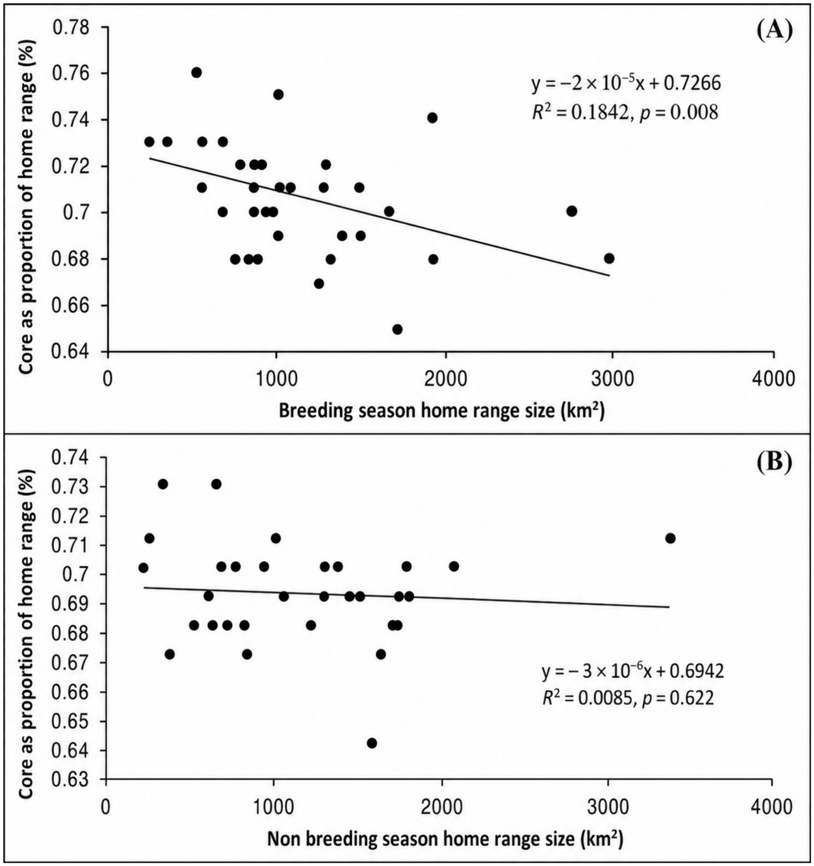
Vulture seasonal home ranges (FK95) clearly had core areas (CAs) of intense use, designated, on average, by the 70.67 ± 2.48% contour during the breeding season and by the 69.13 ± 1.78% contour during the non-breeding season (Table A3, Figure 3). The ICA use index validated the presence of core areas in both seasons, indicating almost three times greater use of core areas than of the periphery of seasonal home ranges (2.79 ± 0.66 and 2.74 ± 0.55, respectively; Table A3). Moreover, the proportion of seasonal home ranges (FK95) classified as core areas was independent of home range size (Figure A1), thereby giving biological meaning to the core areas. Proportionally, breeding season core areas represented a mean of 26.71 ± 6.26% of the breeding season home range size (Table A3) and a mean of 26.08 ± 5.53% of the non-breeding season home range.
The mean seasonal overlap of the spatial parameters SOMCP100, SOMCP95, SOFK95, and SOCA was 959 ± 514 km2, 722 ± 466 km2, 718 ± 395 km2, and 175 ± 76 km2, respectively (Table A4). Proportionally, seasonal overlap of the spatial parameters represented a mean of 45–54% of the annual spatial parameters (49 ± 14%, 54 ± 18%, 46 ± 10%, 45 ± 12%, respectively; Table A4). Furthermore, seasonal overlap of the spatial parameters represented a mean of 62–69% of the respective breeding season spatial parameters, ranging from 18 to 100% (62 ± 23%, 69 ± 25%, 66 ± 18%, 64 ± 21%, respectively; Table A3 and Table A4). Finally, seasonal overlap of the spatial parameters represented a mean of 67–80% of the respective non-breeding season spatial parameters, ranging from 27 to 100% (80 ± 17%, 82 ± 14%, 68 ± 18%, 67 ± 19%, respectively; Table A3 and Table A4).
The results of the LMMs showed significant differences in the size of the examined spatial parameters, whether measured by MCP95 or FK95, in relation to “period” and “artificially provided food”. The independent variable “Age group” was not included in the best models (Table 1), suggesting no differences in spatial parameters among age groups. The dependent variable seasonal CA was retained in the best model only for “artificially provided food”, indicating that the seasonal quantity of artificially provided food strongly affected the seasonal core area size.
Moreover, the LMMs showed significant differences in the magnitude of the overlapped seasonal spatial parameters, as measured by SOMCP95 or SOFK95, in relation to “artificially provided food”. The independent variables “age group” and “period” were not included in the best models, suggesting no differences in spatial parameters among age groups or years (Table 2). The dependent variable seasonal SOCA retained only the “age group” x “artificially provided food” interaction in the best model, indicating that the seasonal quantity of artificially provided food affected seasonal core area overlap across age groups. The model indicated that the juvenile extent of core area overlap was more affected by fluctuations in the amount of “artificially provided food” than the extent of comparable overlap for immatures and adults (Table 2).

3.3. Annual Spatial Parameters

The mean values of the annual spatial parameters MCP100, MCP95, FK95, and CA were 1932 ± 792 km2, 1267 ± 534 km2, 1510 ± 594 km2, and 395 ± 177 km2, respectively (Table A4).
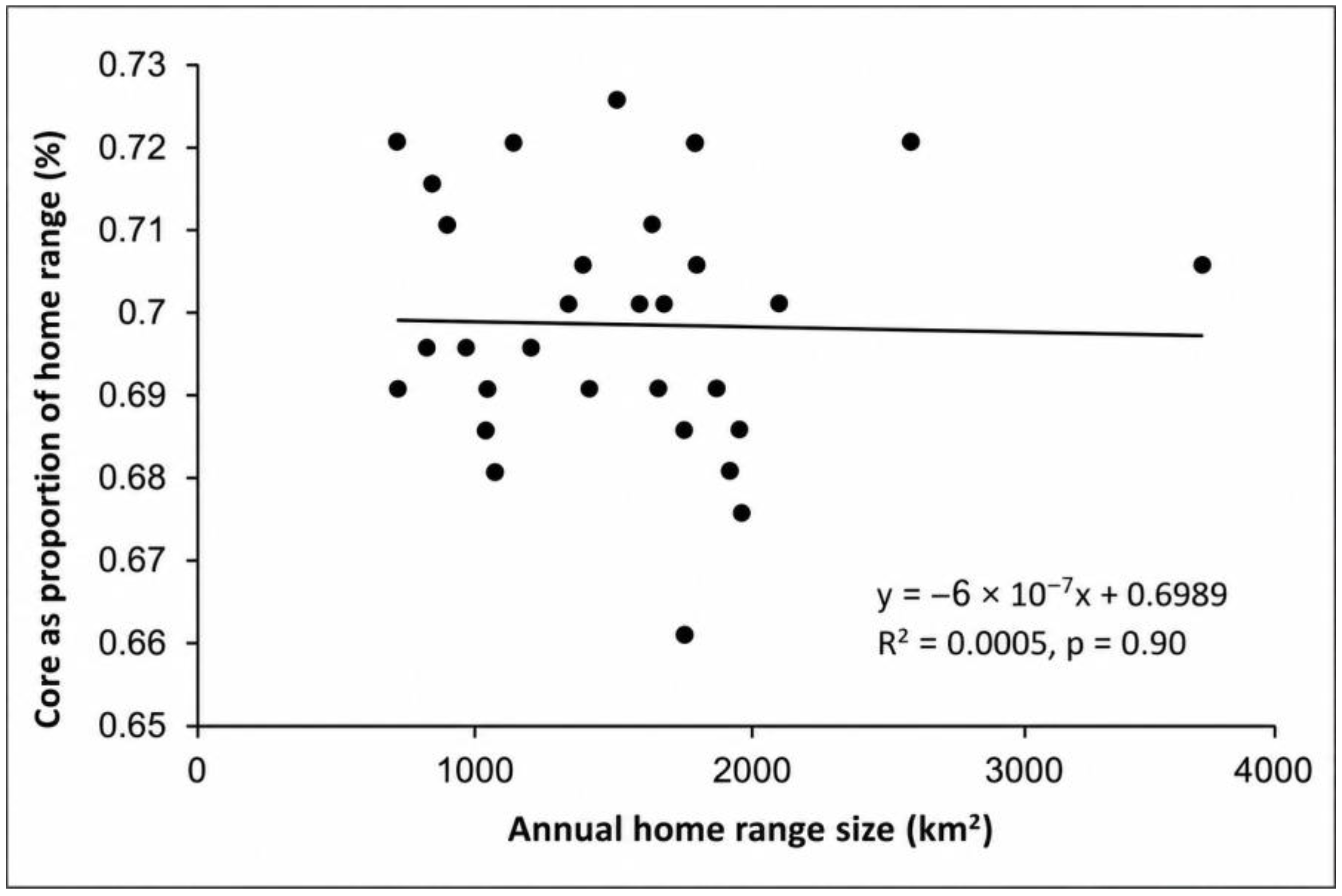
Vulture annual home ranges (FK95) clearly contained areas of intense use, as defined by the preferred core area (CA) algorithm, using the 69.80 ± 1.54% contour (Table A4). The ICA use index confirmed the presence of core areas, yielding values well above one and indicating almost three times more use of core areas than of the periphery of home ranges (2.77 ± 0.45; Table A4). Moreover, the proportion of annual home ranges (FK95) designated as core areas was independent of home range size (p = 0.90; Figure 4), thereby giving biological meaning to the core areas. Proportionally, core areas represented a mean of 26.46 ± 5.34% of the annual home range (Table A4).
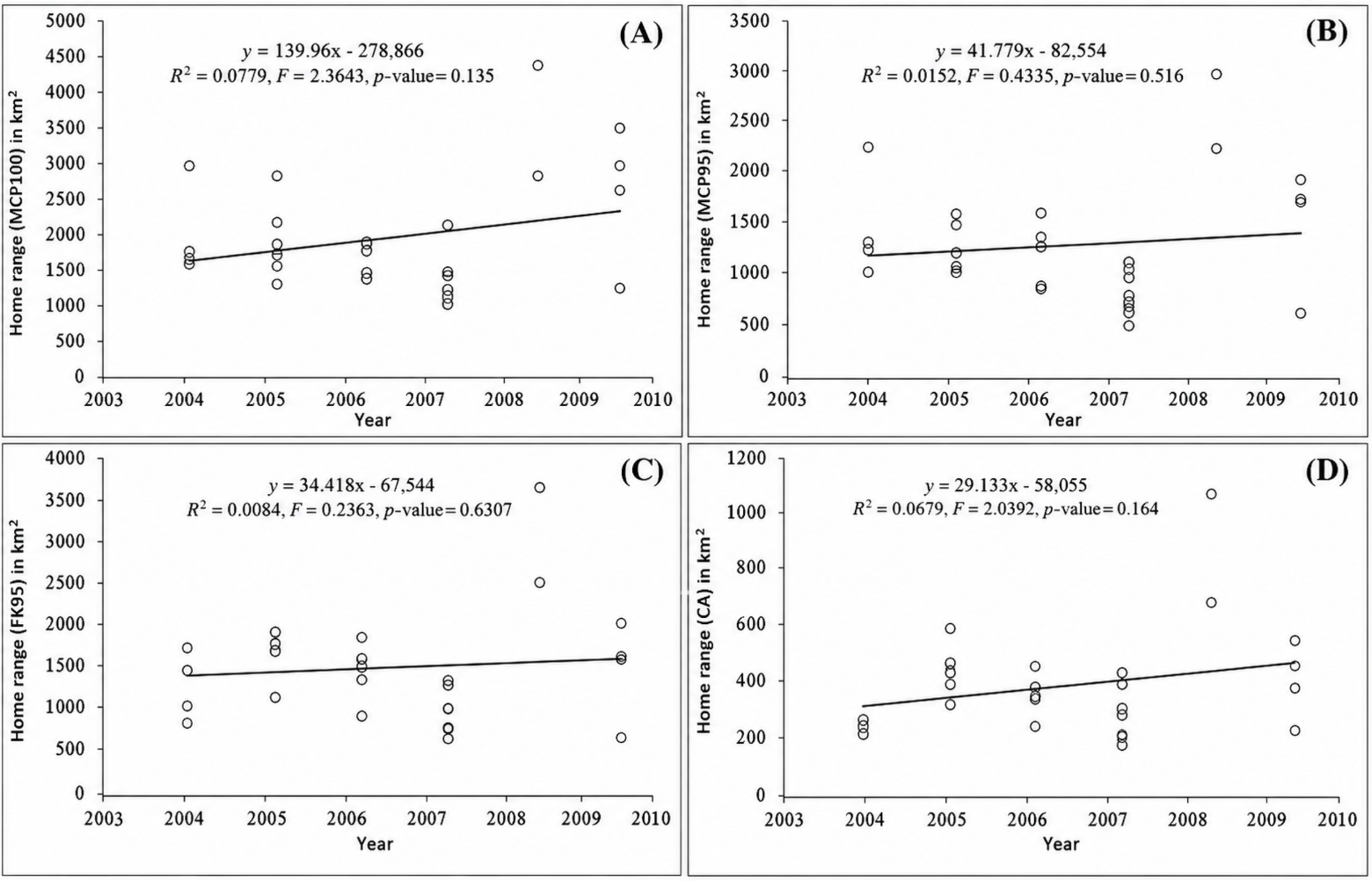
The annual spatial parameters MCP100, MCP95, FK95, and CA did not support the LMMs, either in their original values or after log-transformation. Although there were statistically significant differences between years for these spatial parameters, we pooled them across years because there was no trend over time, indicating that the observed differences were attributable to factors other than year (Table A9, Figure A2). Additionally, the individual had no apparent effect on the annual spatial parameters (Table A10).
Pooling data across years, the age group had no apparent effect on the annual spatial parameters MCP100, MCP95, FK95, and CA (H < 1.608, DF = 2, p > 0.448; Kruskal–Wallis test). Moreover, the annual quantity of “artificially provided food” significantly affected annual spatial parameters, with parameter magnitudes decreasing as the quantity of food increased (MCP100: H = 12.917, DF = 6, p = 0.044; MCP95: H = 15.008, DF = 6, p = 0.020; FK95: H = 17.657, DF = 6, p = 0.007; CA: H = 17.094, DF = 6, p = 0.009). Finally, we found that breeding status (adult breeder, adult non-breeder, or not an adult) had no significant effect on the magnitudes of the annual spatial parameters MCP100, MCP95, FK95, and CA (H < 0.979, DF = 2, p > 0.613; Kruskal–Wallis test).

3.4. Population Home Range and Core Areas

Home ranges and core areas of individual vultures showed considerable overlap (Figure 1). Furthermore, individual ranges, and consequently the overall occupied area, were eccentrically spaced around the colony, with a prevailing northwest orientation (Figure 1). Individual seasonal home range parameters and core areas also overlapped, covering 40–50% of the respective annual parameters (Table A4). The overall spatial parameters for the vulture population during the study period, estimated with MCP100, MCP95, FK95, FK50, and CA, were 5215 km2, 3523 km2, 4970 km2, 943 km2, and 1942 km2, respectively. The population core area was severely underestimated (51%) when the arbitrarily set threshold method (FK50) was used to delineate core areas, compared with our preferred algorithm (CA), which captured a large share of the population range (39%).

4. Discussion

4.1. Methodological Approach

Preliminary analysis of the data informed the selection of appropriate methods and yielded unbiased parameter estimates, thereby safeguarding the quality of the conclusions. Results showed that individual and population home ranges are better described by the 95% Fixed Kernel method because it is not biased by the number of sample locations or tag type. Although determining the appropriate sample size and examining its effect on estimates of the species’ spatial range parameters are critical for identifying potential bias in estimates of space use due to individual variability or inappropriate sampling [47,56,57], they are often neglected [1,5]. This leads to an underestimation of spatial parameters and, in turn, to erroneous inferences about species conservation ecology. Preliminary tests of the appropriate sample size for a location and its effect on spatial range parameters should be conducted in future relevant studies. This approach will help reduce bias in estimates of space use and avoid misleading inferences.
A potential limitation of this study is the unbalanced sample size between tracking technologies, consisting of 12 VHF-tracked and 7 GPS-tracked individuals. This imbalance reflects the historical transition in wildlife telemetry during the 6-year study period. To minimize potential artifactual biases and ensure comparative robustness, we implemented a strict data standardization protocol by downscaling the higher-precision GPS data to match the 2 × 2 km grid cell size of the VHF data. Furthermore, preliminary statistical evaluations indicated no significant differences in spatial parameters by tag type. This suggests that the observed effects of food predictability on home range and core area sizes reflect genuine biological responses rather than variations in monitoring technology. Nonetheless, future long-term studies using standardized, high-resolution tracking across larger cohorts will be valuable for further validating these age-specific and management-driven spatial patterns.
Results also showed that the choice of method for core area estimation can yield different estimates of core area size. The individual annual and seasonal core areas, as well as the population core area, were significantly underestimated when a standard 50% use threshold was applied. The core area is the region where an individual spends the most time relative to the home range periphery [43], making it an invaluable part of the home range. Therefore, it is a mathematically grounded (quantitatively repeatable) and biologically meaningful delineation that is critical for understanding how animals relate to their environment. It also has significant implications for management, conservation, social behavior, and spatial interactions. Our choice of core area delineation used so far in mammalian studies meets the above-mentioned virtues [43], and we have found evidence that the widely used arbitrary 50% contour can substantially underestimate both individual and population core areas [1,5,58,59]. Therefore, we suggest that a more quantitative approach like ours should be used in upcoming raptor movement studies to capture important behavioral aspects, avoid omitting key areas for conservation, and avoid drawing false conclusions about species’ spatial ecology. Nonetheless, future long-term studies using high-resolution GPS telemetry across larger cohorts, paired with direct field observations, will be valuable for further validating the core area boundaries.

4.2. Species-Specific Variation in the Spatial Parameters

Results suggested that the individual seasonal and annual home ranges had core areas of intense use bounded by the 70% contour (rather than the arbitrarily chosen 50% or 80%) [1,5,57,60]. The core area use index validated the seasonal and annual presence of core areas, indicating that vultures use them almost three times as much as the periphery of their home ranges. Unlike those in other studies [5], our core area estimates were uncorrelated with home range estimates, giving biological meaning [44,45] to the core areas and providing a reliable basis for further analysis. Conservation measures, such as supplementary winter feeding for the Bearded Vulture (Gypaetus barbatus) [1] in arbitrarily estimated core areas, require careful evaluation to avoid inadvertently attracting conspecifics and heterospecifics to or near nest sites. Strategic decoupling of winter feeding stations from breeding areas is recommended to mitigate risks of premature territorial defense or localized habitat degradation [1].
We found that seasonal and annual core areas accounted for 26–27% of the respective home ranges. When individual core areas were merged into a population core area, the resulting area covered 39% of the population home range. This indicates that although individual core areas partially overlapped due to central-place foraging behavior, different individuals encompassed spatially distinct areas within their cores. Core areas were neither identical in shape nor completely concentric around the colony. Although they partially overlapped, they were usually oriented toward one or several specific areas, indicating that individuals selected different foraging areas. Similar spatial foraging patterns were recorded in other typical central-place foragers, such as the Griffon Vulture (Gyps fulvus) [5]. These patterns support the idea that vultures have foraging preferences for specific areas and challenge the hypothesis that they forage completely at random.
The seasonal overlap of the spatial parameters covered nearly 50% of the annual parameters and, on average, 65% of the breeding season parameters and 74% of the non-breeding season parameters. This suggests that the area occupied by the individual, and thus the population, is expanded during the breeding season relative to the non-breeding season. This was also shown by the LMMs, which indicated significant seasonal variation in home range size. The home range size of vultures was larger during the breeding season and smaller during the non-breeding season, consistent with findings for the studied species and the Griffon Vulture [5,40]. This may reflect the evolutionary adaptation of vultures to fly passively, soaring and/or gliding by harnessing the atmosphere’s kinetic energy (thermals) [61]. It is known that thermal activity is limited during the colder months of the year, leading to poor flight conditions. This, in conjunction with limited time available for foraging, may have forced vultures to restrict their foraging to areas closer to the colony. Moreover, because breeding individuals must feed themselves and their offspring and meet the increased energy demands of incubation and nestling rearing, they may be compelled to travel extensively to forage successfully.
Unlike other, more territorial vulture species, in which range size increases with age [1], our results showed no differences in seasonal spatial parameters among age groups in the Griffon Vulture. This is consistent with findings on the Griffon Vulture in France and Bulgaria [5,40].
We found that sex had no effect on spatial parameters, whether examined seasonally or annually. This result aligns with expectations for a species that lacks sexual dimorphism and in which both sexes invest equally in reproduction. It is consistent with findings for the species in Spain [32], the Griffon Vulture in France [5], and the Bearded Vulture in southern Africa [1], all of which are marginally sexually dimorphic or sexually monomorphic.
Annual home range size and seasonal overlap of spatial parameters did not vary over the years, indicating that annual variation in home range size was driven by factors other than the year. The demonstrated repeatability of species ranging behavior, despite possible annual variations in ecological conditions, was first reported for the Egyptian Vulture (Neophron percnopterus) [56], but it is not uncommon among other raptor species [58].

4.3. Human-Induced Variation in the Spatial Parameters

We found strong evidence that the predictability of food resources, such as artificially provided food, can shape vultures’ movement ecology. The inclusion of supplementary feeding stations within the core areas of all tracked individuals underscores their importance as predictable food resources. Their close proximity to the breeding colony enables frequent visits at a relatively low energetic cost, while vultures’ social foraging behavior facilitates rapid detection of food availability. Artificially provided food strongly affected the sizes of seasonal home ranges and core areas, as well as their spatial overlap. The same pattern was evident in the annual spatial parameters, with the increasing amount of artificially provided food negatively affecting their magnitude. Artificially provided food is a commonly used management measure to sustain conservation programs for scavengers. Its impact on vultures’ foraging behavior, which has evolved to seek unpredictable resources, has recently been documented [5,56]. It was recently demonstrated that the foraging behavior of the Griffon Vulture, a species closely related to the one studied, could be affected by changes in the predictability of spatial resources (i.e., the presence of feeding sites). Many studies suggest that food availability [62,63] and predictability [5,56] are the primary determinants of avian range ecology, with all other factors being important. Our findings support the idea that the over-provision of artificial food alters vultures’ movement ecology, resulting [16,19,64] in a reduced need to move and thus a smaller home range [5,9]. In the context of our study area, this intensive artificial provisioning presents a complex ecological trade-off rather than a purely positive or negative conservation strategy. On the one hand, it serves as an indispensable safety net that minimizes mortality risks by providing safe food, which is critical for protecting this small, geographically isolated population from poisoning. On the other hand, the resulting shrinkage of home ranges raises valid concerns about long-term behavioral dependence, localized crowding, and the disruption of natural wide-ranging foraging patterns, dispersal and metapopulation dynamics. To reconcile these conflicting outcomes, future conservation management should avoid permanent over-provisioning and instead adopt a more dynamic framework. Introducing temporal and quantitative unpredictability at feeding sites could encourage vultures, particularly younger cohorts, to maintain larger exploratory ranges and preserve their innate foraging plasticity while still benefiting from a baseline population safety net.

4.4. Colony Range and Spatial Pattern

Vultures traveled extensively to forage, and individual annual, seasonal, and population home ranges encompassed former nesting grounds in Bulgaria [23,65]. The population’s foraging range fell within the range of values observed for other Cinereous Vulture populations in Spain (southwestern Spain, Sierra Pelada, 72 pairs, range: 5925 km2; central Spain, Umbría de Alcúdia, 129 pairs, range: 1523 km2; north-central Spain, Alto Lozoya, 100 pairs, range: 6648 km2) and India (winter range: 4680 km2) [32,66,67].
The home ranges and core areas of individual vultures largely overlapped. This possibly reflects the species’ semi-colonial breeding system and its central-place foraging strategy, adopted not only by adults [32] but also by immature individuals and juveniles within the study system. Furthermore, the individual ranges, and consequently the overall occupied area, showed an eccentrically spaced pattern around the colony, with a prevailing northwest orientation. This likely indicates negative selection by the vultures for the eastern and southeastern areas and reflects the topography (flat terrain), land use (agricultural areas), intensive human presence, and limited thermal lifts in those areas.
The juveniles and immature individuals in our study colony had restricted home ranges for multiple consecutive years. In this context, it is extremely unlikely that they would disperse or migrate as individuals from other populations do. The foraging range of these age groups in our area is 1000–1300 times smaller than that of the same age classes in Alto Lozoya, north-central Spain [68]. Additionally, juveniles from the eastern population (Turkey, Eskisehir colony, 400 km away; Georgian and Armenian colonies, >1500 km away) migrate to Iran and Saudi Arabia [68,69], unlike individuals in our study population. We suggest that this might reflect the accumulation of mutations in the Balkan vulture population due to historical isolation that differentiates it from the others [55]. Alternatively, the over-provision of artificial food at stable positions alters vultures’ foraging behavior [16,19,64], resulting in less need to move and thus a smaller home range [5,9].

5. Conclusions

Careful selection of home range and core area estimators, along with unbiased parameter estimates, safeguards the quality of any conclusions drawn regarding vulture management, conservation, and spatial ecology. Vultures have foraging preferences for specific areas and are unlikely to forage completely at random. Their range varies seasonally, reflecting vultures’ evolutionary adaptations for passive flight, foraging time constraints, and heightened energetic demands in certain seasons. Vultures use core areas three times as much as the periphery of their home ranges. These areas must be designated as conservation priority areas for the species, excluded from wind farm development, and conservation efforts must be intensified.
Home range size and core areas did not differ among age groups in vultures. This deviates from the movement behavior the species exhibits in Spain and might be a side effect of the over-provision of artificial food in a specific, restricted area near the colony. Results demonstrated repeatability in the species’ ranging behavior over the years. From a conservation perspective, this enables the establishment of effective, long-term conservation measures if ecological conditions remain unchanged. On the other hand, it also allows species’ range spatial modeling to be used in research that requires combining data from different periods or assumes a high degree of repeatability in space use, such as sensitivity mapping [30,31,70,71]. Moreover, the results underscored the importance of artificial, highly predictable food provision in shaping the movement ecology of this necrophagous species. Actions that ensure the availability of safe food are essential for the preservation of this and other endangered vultures. We suggest that supplementary feeding management should be gradually diversified to simulate natural carrion availability by using multiple small feeding sites and supplementing them unpredictably with small amounts of high quality food.
Juveniles and immature individuals are extremely unlikely to disperse or migrate as individuals from other populations do, which may reflect that the over-provision of artificial food alters vultures’ movement behavior. Therefore, the conservation strategy for this endangered species in Greece might need to incorporate the translocation of individuals to carefully planned reintroduction projects in other areas.

Author Contributions

Conceptualization, D.V. and V.K.; methodology, D.V., K.Z. and V.K.; software, D.V.; validation, D.V.; formal analysis, D.V.; investigation, D.V.; resources, D.V.; data curation, D.V. and V.L.; writing—original draft preparation, D.V., K.Z., V.L. and V.K.; writing—review and editing, D.V., K.Z., V.L. and V.K.; visualization, D.V.; supervision, V.K.; project administration, V.K. and D.V.; funding acquisition, D.V. and V.K. All authors have read and agreed to the published version of the manuscript.

Funding

Fieldwork and equipment were funded primarily by (a) WWF Greece through the LIFE-Nature project Conservation of Birds of Prey in the Dadia Forest Reserve, Greece (LIFE02 NAT/GR/8497), and (b) the Recreation and Development Union in Bulgaria through the PHARE Project BG 2004/016-782.01.03.07, Promotion of Nature Protection and Sustainable Development across the Border (Bulgaria–Greece): Flying over the Borders. The work of D.P.V. was partially supported by the Hellenic Republic through a granted leave covering 60% of the author’s official working time during the preparation of his PhD thesis. The leave was granted by Decisions No. 5575/11 April 2013 and No. 11445/17 August 2016 of the General Secretary of the Decentralized Administration of Macedonia and Thrace. Natural Research Ltd. supported the dissemination of the research results by supporting the PhD studentship of D. Vasilakis, entitled Movement Ecology and Feeding Behaviour of an Endangered Vulture Species (Aegypius monachus) in Thrace, was provided through a donation (Grant No. Ε.312/2014).

Institutional Review Board Statement

The tagging process was undertaken under specific permission from the Ministry of Environment, Energy, and Climate Change (Greece) and the Hellenic Ringing Center (Approval Code: 99110/4096 and the Approval Date: 15 October 2008).

Data Availability Statement

The data presented in this study is available on request from the corresponding author.

Acknowledgments

We sincerely thank D. Philip Whitfiel, for invaluable scientific guidance, mentorship, and unwavering encouragement. We are grateful to K. Poirazidis, T. Skartsi, P. Babakas, J. Elorriaga, E. Kret, B. Cárcamo S. Stoychev and S. Avramov for their valuable contribution to fieldwork and descusions, as well as to the numerous anonymous but dedicated European Voluntary Service (WWF) volunteers taking part in fieldwork. Fieldwork was also conducted by the Bulgarian Society for the Protection of Birds and Green Balkans. Fieldwork and equipment were funded primarily by WWF Greece and also by the Recreation and Development Union in Bulgaria (Life and Phare projects).

Conflicts of Interest

The authors declare no conflicts of interest. The funders had no role in the design of the study; in the collection, analyses, or interpretation of data; in the writing of the manuscript; or in the decision to publish the results.

Abbreviations

The following abbreviations are used in this manuscript:
AAdult
ABAdult breeder
ANBAdult non-breeder
BSBreeding Season
CACore Area
CICA Contour indicating the core area
DFDegrees of freedom
DLS NPDadia-Lefkimi-Soufli National Park
FFledgling
Fe Female
FKFixed Kernel
Fr2Test statistic coefficient of determination
GSM Global System for Mobile Communications
GPSGlobal Position System
HTest statistic for Kruskal–Wallis test
ICAIntensity of core area use index
J Juvenile
I Immature
LMMsLinear Mixed Models
LCILower Confidence Interval
MMale
MCPMinimum Convex Polygon
NNumber of Individuals
NANonadult
NBSNon-breeding Season
NRDtest for the deviation from normality of the residual distribution with the Shapiro–Wilk normality test
NsNumber of season (breeding/non-breeding)
PSignificance
rsSpearman’s rank-order correlation a nonparametric option
rs2coefficient of determination
STest statistic Spearman’s rank-order correlation
SLSample locations were home range size rich an asymptote
SOBefore parameters MCP100, MCP95, FK95 and CA stands for “seasonal overlap”
SOCASeasonal Overlap Core Area
SOFKSeasonal Overlap Fixed Kernel
SOMCPSeasonal Overlap Minimum Convex Polygon
SDStandard Deviation
SEStandard Error
TTest statistic
TLTotal location
UMann–Whitney test statistic
UCIUpper Confidence Interval
UnUnknown
UKUnited Kingdom
VHFVery High Frequency
W1Vulture weight
W2Backpack weight

Appendix A

Table A1. Information for the 19 Cinereous Vultures tracked and the number of locations that were analyzed for the period 2004 to 2009.
NIndividual
Vulture
Code
Tag
Type
Vulture SexTotal
Number
of Locations
Monitoring PeriodTracking Duration
(Months)
Backpack Weight
StartEndNsAge ClassesTotalW1 (gr)W2 (gr)W1/W2
(%)
F J I A
1102h15VHFMale10891/2/200431/1/20088 12364873501552.11
2103H10VHFFemale13321/2/200431/1/20088 12364881501551.90
3104H34VHFFemale3545/5/200431/1/20083 3.8 1215.87650951.24
4105h35VHFFemale2031/2/200431/8/20041 779100951.04
5106H09VHFMale2451/2/200431/1/20052 121279501551.95
6107H33VHFFemale10251/2/200431/1/20088 48489100951.04
7108H25VHFMale9061/2/200531/1/20066 1224 3682501551.88
8109H37VHFMale19820/9/200431/8/200524.37 11.378501551.97
9110H40VHFFemale561/2/200531/8/20051 7 770001552.21
10111H12VHFMale92120/9/200431/1/200874.31224 40.37300951.30
11112H38VHFFemale1651/2/200531/1/20062 12 1284001551.85
12114H61VHFUnknown2831/2/200731/1/20082 12 126550951.45
13113H88GPS PlusUnknown4941/2/200731/8/20083 1271980001752.19
143664H71GPS PlusUnknown10231/2/200831/3/20093 1221481501752.15
153688H38GPS PlusUnknown9821/2/200831/3/20093 141481501752.15
162021H83GPS GSMUnknown350614/10/200821/4/20092 6.16.175302202.92
172022H67GPS GSMUnknown302714/10/200810/4/20092 3.52.3 5.883502202.63
182023H45GPS GSMUnknown244831/10/200821/3/20092 4.6 4.675002202.93
192024H56GPS GSMUnknown334231/10/200810/5/20092 6.3 6.386002202.56
Average 5M:6F:8U1137 44.38.712.118.019.379441561.97
SD 1115 20.03.87.715.915.9657450.57
Total 21,599 678.669.3109.2180.1367.2
N: Number of Individuals, Ns: Number of season (breeding/non-breeding), F: Fledgling, J: Juvenile, I: Immature, A: Adult, W1: Vulture weight, W2: Backpack weight.
Table A2. Annual and seasonal amounts (metric tons) of dead livestock artificially provided in feeding sites called “vulture restaurants”. See Figure 1 for feeding sites localities in relation to the colony.
YearSeasonTotal
BSNBS
200416.7813.4330.21
200518.559.6628.21
200617.6518.9636.61
200716.6319.2135.84
200818.0617.3235.38
200916.68¯¯
Average17.3915.7233.25
SD0.814.103.78
Total104.3478.58166.24
BS: breeding season (February to August), NBS: non-breeding season.
Table A3. Individual characteristics for the 19 Cinereous Vultures (Aegypius monachus) tracked and the number of location that were analyzed for the period 2004 to 2009 as well as seasonal home range and core area estimates in Thrace, northeast Greece. Home range was estimated using 100% Minimum Convex Polygon (MCP; MCP100), the 95% MCP (MCP95), the 95% fixed kernel (FK95) and the 50% fixed kernel (FK50) while core areas (CAs) calculated after Vander Wal and Rodgers’ algorithm [43].
Vulture/
Seasons
Individual
Vulture
Code
Tag
Type
Vulture SexAge ClassesBreeding StatusYearSLTLMCP100
(km2)
MCP95
(km2)
FK95
(km2)
CICA
(%)
CA
(km2)
ICAFK50
(km2)
Breeding Season
1102H15VHFMINA20041331871908.651654.08963.9275189.473.8285.67
2103H10VHFFeINA20042543211742.02997.47748.0472239.602.25116.30
3104H34VHFFeJNA200490129809.05532.32339.5773106.182.3352.39
4105H35VHFFeAANB20041562031370.79656.41491.267686.034.3432.19
5106H09VHFMAAB20041521781134.72812.82477.977693.393.8932.96
6107H33VHFFeAAB20041441791241.71827.84651.4373122.183.8950.80
7102h15VHFMAANB20051031031467.771102.72838.1172231.712.6079.50
8103H10VHFFeAAB200586114897.39618.57846.3168273.952.10147.25
9107H33VHFFeAAB200554721269.691014.651335.5969297.013.10150.02
10108H25VHFMJNA200555851284.43843.53929.7170179.143.6371.06
11109H37VHFMJNA20051381381685.98953.04870.7772197.873.1775.96
12110h40VHFFeJNA200556561326.091006.031646.3265535.152.00347.12
13111H12VHFMJNA200556851106.02887.641265.0568298.692.88138.02
14112H38VHFFeJNA2005501061058.61960.511203.9467250.823.22104.76
15102H15VHFMAAB2006902001672.401296.211438.2469385.842.57149.77
16103H10VHFFeAAB2006781931017.94739.53900.0970229.192.7598.31
17107H33VHFFeAANB20061061991579.73898.11977.1271267.332.6151.89
18108H25VHFMINA2006722081357.08871.50826.8771181.883.2377.95
19111H12VHFMINA2006822111857.97582.181860.6668460.612.75235.02
20102H15VHFMAANB2007931681036.47788.68932.4270314.352.0899.36
21103H10VHFFeAANB20071042011039.73696.59796.5268283.241.91156.28
22104H34VHFFeAANB200771160952.67516.13722.1568219.952.23143.75
23107H33VHFFeAANB2007881901978.10986.991225.1071268.173.24145.78
24108H25VHFMINA2007952381412.86745.371041.9071234.643.15121.67
25111H12VHFMINA2007952241116.60582.17642.8970186.992.41104.10
26113H88GPS PlusUnINA20071191731429.48943.30966.7069441.161.51131.79
27114H61VHFUnJNA20071012001156.29747.54828.4770188.643.0790.30
283664H71GPS PlusUnINA20082323721980.311588.131841.4274453.172.09182.96
293688H38GPS PlusUnAANB20081593524396.212569.262655.0770740.513.01322.00
30113H88GPS PlusUnAANB200850165525.6586.27218.527376.192.5139.48
312021H83GPS GSMUnAANB200922716212429.281341.551427.3571420.972.86205.29
322022H67GPS GSMUnINA200912412143406.951673.691238.8872420.432.92205.95
332023H45GPS GSMUnINA20092278811045.27562.61528.8371187.002.4166.24
342024H56GPS GSMUnINA200926817872617.571705.491595.5870299.612.12101.89
353664H71GPS PlusUnAANB2009792311753.65443.71529.8173135.042.0158.10
363688H38GPS PlusUnAANB2009702302337.262213.842860.9268666.843.73216.64
Average 6115.47315.941566.73984.621073.9970.67282.302.79124.68
SD 59.81404.30747.89499.66574.102.48154.190.6674.13
Subtotal26VHF:10GPS12M:13F:11U7J:11I:18A6AB:12ANB:18NA6415711,374
Non-breeding season
1102H15VHFMINA200470842485.421835.811444.6569271.923.67147.20
2103H10VHFFeINA2004110128811.60626.13656.4970153.283.0065.45
3106H09VHFMAAB200450671264.991071.261392.8069224.883.4199.29
4107H33VHFFeAAB200468741370.381203.08956.0671248.412.73151.14
5109H37VHFMF *NA20045460666.58393.46800.4867225.622.38142.86
6111H12VHFMFNA20045461369.96139.79249.837184.372.1023.23
7102H15VHFMAANB20051051291976.201590.541679.2669439.672.64205.43
8103H10VHFFeAAB2005771142754.131471.521720.3670373.633.22201.99
9107H33VHFFeAAB2005821021840.181148.451654.7468414.202.72218.50
10108H25VHFMJNA2005711201248.82942.081569.6467362.642.90193.83
11111H12VHFMJNA200550711011.35918.891517.7064581.661.67334.86
12112H38VHFFeJNA200559591378.431030.141637.6268334.253.33172.09
13102H15VHFMAAB200667118785.47610.891023.9169206.843.42114.89
14103H10VHFFeAAB2006861321321.31672.751173.6668315.712.53200.44
15107H33VHFFeAANB2006501261240.591072.171246.9969276.103.12112.94
16108H25VHFMINA200665141560.48331.00604.4068230.881.78114.64
17111H12VHFMINA200691160745.27456.13688.9068200.082.34103.76
18102H15VHFMAANB2007581001343.82943.821240.3170270.153.21165.15
19103H10VHFFeAANB200756129785.82421.85790.3068202.022.66121.17
20104H34VHFFeAANB20075065298.71132.42209.457052.062.8216.48
21107H33VHFFeAANB200750831034.55801.70737.9670169.663.04103.46
22108H25VHFMINA200767114261.18178.86355.2567116.462.0465.54
23111H12VHFMINA200750109703.31390.76587.1169186.922.1793.36
24113H88GPS PlusUnINA200750156505.76193.24491.9668151.062.2161.40
25114H61VHFUnJNA20075083597.78401.96328.517360.853.9429.57
262021H83GPS GSMUnAANB200827918852301.311873.701729.1769498.362.79287.85
272022H67GPS GSMUnINA200811118131513.191321.631311.4270355.563.39206.55
282023H45GPS GSMUnINA200818215671162.08533.73622.2473208.142.3964.03
292024H56GPS GSMUnINA20081251555965.40823.85902.4670239.512.58109.84
303664H71GPS PlusUnINA2008964202636.332114.961988.1470498.082.18227.00
313688H38GPS PlusUnAANB2008894002867.402644.503209.8071671.362.64226.05
Average 81.35329.841251.86912.621113.6069.13278.212.74141.29
SD 46.87546.74735.83622.17636.621.78148.440.5576.54
Subtotal24VHF:7GPS13M:10Fe:8Un2F:4J:11I:14A6AB:8ANB:17NA5252210,225
Average 99.69322.371421.05951.311092.3169.96280.412.77132.37
SD 56.48471.81753.49556.47599.502.31150.430.6175.15
Total 50VHF:17GPS25M:23Fe:19Un2F:11J:22I:32A12AB:20ANB:35NA 667921,599
VHF: very high frequency, GPS: Global position system, Fe = Female, M = Male, Un = Unknown, F = fledglings, J = juvenile, I = Immature, A = Adult, AB: Adult breeder, ANB: Adult non-breeder, NA: Nonadult, SL: Sample locations were home range size rich an asymptote, TL: Total location, CICA: Contour indicating core area, ICA: intensity of core area use index, Breeding season: February to August; * Fledglings were merge with Juvenile.
Table A4. Individual characteristics for the 19 Cinereous Vultures (Aegypius monachus) tracked for the period 2004 to 2009, as well as annual home range and core area estimates in Thrace, northeast Greece. Annual home range values were estimated by merging the seasonal 100% Minimum Convex Polygon MCP (MCP100), the 95% MCP (MCP95), the 95% fixed kernel (FK95), the 50% fixed kernel (FK50), and the core areas (CAs). Seasonal overlaps of the mentioned spatial parameters are also presented.
Vulture/
Years
Individual
Vulture
Code
Tag
Type
Vulture SexAge ClassesBreeding StatusYearMCP100 (km2)MCP95 (km2)FK95 (km2)FK50 (km2)CICA (%)CA (km2)ICASOMCP100 (km2)SOMCP100 (%) *SOMCP95 (km2)SOMCP95 (%) *SOFK95 (km2)SOFK95 (%) *SOCA (km2)SOCA (%) *
1102h15VHFMINA20042965.312216.851751.34147.2072.00287.163.741428.7648.181273.0457.43657.2337.53174.2360.67
2103H10VHFFeINA20041742.021022.87903.59124.1671.00269.312.62811.6046.59601.0058.76500.9455.44123.5845.89
3106H09VHFMAAB20041669.811300.491491.36103.0672.50236.073.65729.8043.71583.7144.88379.4125.4482.2034.82
4107H33VHFFeAAB20041596.641236.811123.04151.1472.00248.743.311015.4563.60794.1164.21484.4543.14121.8548.99
5102h15VHFMAANB20052157.441598.141767.95344.9370.50454.562.621286.5359.631095.0268.52749.4242.39216.8247.70
6103H10VHFFeAAB20052829.651471.521836.00239.0769.00455.192.66821.8729.04618.5742.04730.6739.80192.3842.26
7107H33VHFFeAAB20051869.111203.141911.69203.4168.50477.442.911240.7866.38960.2179.811078.6456.42233.7748.96
8108H25VHFMJNA20051673.801058.011729.09188.8468.50399.003.27859.1251.33727.4368.75770.2744.55142.7735.78
9109H37VHFMJNA20051757.791020.391196.64264.4569.50338.602.77598.9934.08325.7931.93474.6139.6684.8825.07
10111H12VHFMJNA20051288.291073.541727.84218.6366.00602.682.27828.9364.34733.3468.311054.9261.05277.6746.07
11112H38VHFFeJNA20051540.571213.001925.99237.6467.50430.323.27897.1958.24776.8264.04915.5747.54154.7535.96
12102h15VHFMAAB20061740.681366.561636.09130.4869.00400.412.99717.4741.22541.4039.62826.0650.49192.2748.02
13103H10VHFFeAAB20061458.55892.211406.94250.2369.00363.402.64880.7060.38520.0858.29666.8147.39181.5149.95
14107H33VHFFeAANB20061817.861267.371575.59160.3370.00356.802.861003.3855.20702.2855.41648.5241.16186.6452.31
15108H25VHFMINA20061385.41872.29969.35219.6269.50265.572.50532.1538.41330.1737.85461.9147.65147.1855.42
16111H12VHFMINA20061861.561594.371879.16118.8768.00470.952.54740.2139.76452.3628.37670.4135.68189.7440.29
17102h15VHFMAANB20071460.801055.841327.35104.1470.00402.712.65919.4962.94676.6764.09845.3863.69181.7845.14
18103H10VHFFeAANB20071090.08698.771065.63141.3468.00325.602.29733.7867.31419.6860.06521.1948.91159.6649.04
19104H34VHFFeAANB20071024.44525.67737.50133.6569.00228.622.52226.9522.15122.7623.35194.0926.3243.3918.98
20107H33VHFFeAANB20072110.921120.641378.16151.5870.50301.663.14900.9942.68668.0759.62584.9042.44136.1745.14
21108H25VHFMINA20071412.87745.371048.60153.8669.00235.492.60261.1918.49178.8724.00348.5433.24115.6249.10
22111H12VHFMINA20071200.02635.71832.27198.0069.50220.822.29619.9051.66337.2353.05397.7347.79153.0969.33
23113H88GPS PlusUnINA20071460.22966.421046.44204.6168.50446.621.86474.7732.51170.1317.60412.2139.39145.6132.60
24114H61VHFUnJNA20071246.28807.78857.46177.3371.50200.423.51507.9840.76340.7442.18299.5234.9349.0724.48
253664H71GPS PlusUnINA20082842.412199.142515.53279.2772.00692.692.141773.1662.381505.2268.451314.0252.24258.5637.33
263688H38GPS PlusUnAANB20084426.212877.073605.89395.6270.501076.392.822836.3864.082336.2081.202258.9962.65335.4831.17
272021H83GPS GSMUnAANB20092977.611913.882051.11259.3570.00559.022.831752.9758.871301.3768.001105.4153.89360.3164.45
282022H67GPS GSMUnINA20093490.021723.021621.31153.6671.00467.173.161454.1641.671272.2073.84929.0057.30308.8266.10
292023H45GPS GSMUnINA20091250.58626.41730.04103.2272.00251.182.40955.9476.44473.4775.58421.0357.67143.9657.31
302024H56GPS GSMUnINA20092625.841705.491656.80338.9470.00390.332.35957.1336.45823.8448.31841.2350.77148.8038.12
Average 1932.431266.961510.19196.5569.80395.162.77958.9249.28722.0654.25718.1046.22174.7544.88
SD 791.96534.28594.0274.251.54176.550.45513.7714.47465.6217.52395.479.9976.0312.22
Total 23VHF:7GPS12M:10F:8U5J:11I:14A6AB:8ANB:16NA6
VHF: very high frequency, GPS: Global position system, Fe = Female, M = Male, Un = Unknown, J = juvenile, I = Immature, A = Adult, AB: Adult breeder, ANB: Adult non-breeder, NA: Nonadult, CICA: Contour indicating core area, ICA: intensity of core area use index, SO: before parameters MCP100, MCP95, FK95 and CA stands for “seasonal overlap”. * The seasonal overlap of the parameters MCP100, MCP95, FK95, and CA is expressed as a percentage of the annual total.
Table A5. Results of the correlation analysis of the spatial parameters with the location sample size used in their estimation.
PeriodSpatial ParametersStatistical Parameters
rsDFrs2SpN
AnnualMCP1000.520280.27021480.00130
MCP950.460280.21024270.00530
FK950.140280.01938570.23030
FK500.005280.00045160.50930
CA0.150280.02238230.22030
BSMCP1000.450340.20342700.00336
MCP950.289340.08455220.04436
FK950.049340.00281520.61236
FK500.100340.01085460.71936
CA0.052340.00373670.38236
NBSMCP1000.512290.26224200.00231
MCP950.478290.22925870.00331
FK950.418290.17528860.01031
FK500.425290.18128520.00931
CA0.456290.20826960.00531
rs: Spearman’s rank-order correlation a nonparametric option, DF: degrees of freedom, rs2: coefficient of determination, S: Test statistic Spearman’s rank-order correlation, p: level of significance, N: number of individuals/years or individual/seasons, BS: Breeding season, NBS: Non-breeding season. MCP100: maximum area of activity used, including outlier locations, MCP95: maximum area of activity used, excluding outlier locations, FK95: indicates the area of the home range within which the individual spends 95% of its time, FK50: core area delineation using the fixed 50% fixed kernel contour value threshold, CA: core area estimated by definition algorithm [43].
Table A6. Results of the analysis of the effect of different tag types on the spatial parameters.
PeriodSpatial ParametersStatistical Parameters
HDFpN
AnnualMCP1007.1812.0000.02830
MCP956.8372.0000.03330
FK955.6042.0000.06130
FK504.9592.0000.08430
CA1.7312.0000.42130
BSMCP10011.5012.0000.00336
MCP954.8752.0000.08736
FK954.4742.0000.10736
FK503.2572.0000.19636
CA4.7612.0000.09236
NBSMCP1006.4532.0000.04031
MCP956.9852.0000.03031
FK955.8622.0000.05331
FK504.5852.0000.10131
CA6.0782.0000.04831
H: test statistic for the Kruskal–Wallis chi-squared test, DF: degrees of freedom, p: level of significance, N: number of individual/years or individual/seasons, BS: Breeding season, NBS: Non-breeding season. MCP100: maximum area of activity used, including outlier locations, MCP95: maximum area of activity used, excluding outlier locations, FK95: indicates the area of the home range within which the individual spends 95% of its time, FK50: core area delineation using the fixed 50% fixed kernel contour value threshold, CA: core area estimated by the definition algorithm [43].
Table A7. Results of the analysis of the effect of sex on the spatial parameters.
PeriodSpatial ParametersStatistical Parameters
UpN
AnnualMCP100620.92324
MCP95520.62824
FK95580.92324
FK50680.62824
CA601.00024
BSMCP100510.15225
MCP95660.53825
FK95650.50325
FK50890.57425
CA820.85225
NBSMCP100870.18623
MCP95800.37623
FK95720.69323
FK50700.78423
CA680.87923
U: test statistic for the Mann–Whitney test, p: level of significance, N: number of individuals/years or individual/seasons, BS: Breeding season, NBS: Non-breeding season, MCP100: maximum area of activity used including outlier locations, MCP95: maximum area of activity used excluding outlier locations, FK95: indicate the area of the home range within which individual spends 95% of its time, FK50: core area delineation using the fixed 50% fixed kernel contour value threshold, CA: core area estimated by the definition algorithm [43].
Table A8. Results of the analysis of the effect of the core area estimation method on the core area size.
PeriodSpatial Parameters (km2) Statistical Parameters
CA (Mean)CA (SD)FK50 (Mean)FK50 (SD)CAA (%)UpN
Annual395.165176.551196.55375.51850.2608150.00030
BS282.305154.191124.68174.13355.83511030.00036
NBS278.205148.442141.29076.54149.2147710.00031
CA: core area estimated by the definition algorithm [43], FK50: core area delineation using the fixed 50% fixed kernel contour value threshold, CAA: core area underestimation = (((CA-FK50)/CA) × 100), U: test statistic for the Mann–Whitney test, p: level of significance, N: number of individual/years or individual/seasons, BS: Breeding season, NBS: Non-breeding season.
Table A9. Results trend and effect analysis of the year with the annual spatial parameters.
Spatial ParametersTrend AnalysisEffect Analysis
rs2Fr2pNHDFp
MCP1000.0782.3640.1353012.90650.024
MCP950.0150.4340.5163014.35850.013
FK950.0080.2360.6313015.92950.007
CA0.0682.0390.1643016.06150.007
rs2: coefficient of determination, Fr2: Test statistic coefficient of determination, p: level of significance, N: number of individual/years, H: test statistic for Kruskal–Wallis test, DF: degrees of freedom. MCP100: maximum area of activity used, including outlier locations, MCP95: maximum area of activity used excluding outlier locations, FK95: indicates the area of the home range within which the individual spends 95% of its time, CA: core area estimated by the definition algorithm [43].
Table A10. Results of the effect analysis of the individual on the annual spatial parameters.
Spatial ParametersStatistical Parameters
HDFp
MCP10019.956160.222
MCP9521.554160.158
FK9518.417160.300
CA17.418160.359
H: test statistic for Kruskal–Wallis test, DF: degrees of freedom, p: level of significance, MCP100: maximum area of activity used including outlier locations, MCP95: maximum area of activity used excluding outlier locations, FK95: indicates the area of the home range within which the individual spends 95% of its time, CA: core area estimated by definition algorithm [43].
Figure A1. Relationship between contour values that defined the boundary of the seasonal core area (i.e., the proportion of the home range where the animal maximizes its time in relation to the periphery) and seasonal home range size. The proportion of the seasonal home ranges (FK95) designated as core areas was independent of the seasonal home range size (A) for the breeding season and (B) for the non-breeding season.
Diversity 18 00466 g0a1
Figure A2. Trend analysis of the annual spatial parameters over the years. The open circles indicate the values of the different parameters for the different individuals across the years, and the solid line indicates the fitted trend line. The line equation can be seen, as well as the coefficient of determination, the test statistic, and the level of significance. (A) MCP100 indicates the maximum area of activity used, including outlier locations, (B) MCP95 indicates the maximum area of activity used, excluding outlier locations, (C) FK95 indicates the area of the home range within which the individual spends 95% of its time, and (D) CA core area estimated by the definition algorithm [43].
Diversity 18 00466 g0a2

References

  1. Krüger, S.; Reid, T.; Amar, A. Differential Range Use between Age Classes of Southern African Bearded Vultures Gypaetus barbatus. PLoS ONE 2014, 9, e114920. [Google Scholar] [CrossRef] [Scilit] [PubMed]
  2. Braham, M.; Miller, T.A.; Duerr, A.E. Home in the Heat: Dramatic Seasonal Variation in Home Range of Desert Golden Eagles Informs Management for Renewable Energy Development. Biol. Conserv. 2015, 186, 225–232. [Google Scholar] [CrossRef] [Scilit]
  3. Jaeger, A.; Goutte, A.; Lecomte, V.J.; Richard, P.; Chastel, O.; Barbraud, C.; Weimerskirch, H.; Cherel, Y. Age, Sex, and Breeding Status Shape a Complex Foraging Pattern in an Extremely Long-Lived Seabird. Ecology 2014, 95, 2324–2333. [Google Scholar] [CrossRef] [Scilit] [PubMed]
  4. García-Ripollés, C.; López-López, P.; Urios, V. Ranging Behaviour of Non-Breeding Eurasian Griffon Vultures Gyps fulvus: A GPS-Telemetry Study. Acta Ornithol. 2011, 46, 127–134. [Google Scholar] [CrossRef] [Scilit]
  5. Monsarrat, S.; Benhamou, S.; Sarrazin, F.; Bessa-Gomes, C.; Bouten, W.; Duriez, O. How Predictability of Feeding Patches Affects Home Range and Foraging Habitat Selection in Avian Social Scavengers? PLoS ONE 2013, 8, e53077. [Google Scholar] [CrossRef] [Scilit] [PubMed]
  6. Martínez-Abraín, A.; Tavecchia, G.; Regan, H.M.; Jiménez, J.; Surroca, M.; Oro, D. Effects of Wind Farms and Food Scarcity on a Large Scavenging Bird Species Following an Epidemic of Bovine Spongiform Encephalopathy. J. Appl. Ecol. 2012, 49, 109–117. [Google Scholar] [CrossRef] [Scilit]
  7. Linnell, J.D.C.; Andersen, R.; Kvam, T.; AndrÉn, H.; Liberg, O.; Odden, J.; Moa, P.F. Home Range Size and Choice of Management Strategy for Lynx in Scandinavia. Environ. Manag. 2001, 27, 869–879. [Google Scholar] [CrossRef] [Scilit] [PubMed]
  8. Plotz, R.D.; Grecian, W.J.; Kerley, G.I.H.; Linklater, W.L. Standardising Home Range Studies for Improved Management of the Critically Endangered Black Rhinoceros. PLoS ONE 2016, 11, e0150571. [Google Scholar] [CrossRef] [Scilit] [PubMed]
  9. Margalida, A.; Colomer, M.A.À. Modelling the Effects of Sanitary Policies on European Vulture Conservation. Sci. Rep. 2012, 2, 753. [Google Scholar] [CrossRef] [Scilit] [PubMed]
  10. Dodge, S.; Bohrer, G.; Bildstein, K.; Davidson, S.C.; Weinzierl, R.; Bechard, M.J.; Barber, D.; Kays, R.; Brandes, D.; Han, J.; et al. Environmental Drivers of Variability in the Movement Ecology of Turkey Vultures (Cathartes aura) in North and South America. Phil. Trans. R. Soc. B 2014, 369, 20130195. [Google Scholar] [CrossRef] [Scilit] [PubMed]
  11. Mundy, P.J. The Comparative Biology of Southern African Vultures; Vulture Study Group: Johannesburg, South Africa, 1982; ISBN 0125105851. [Google Scholar]
  12. Meretsky, V.J.; Snyder, N.F.R. Range Use and Movements of California Condors. Condor 1992, 94, 313–335. [Google Scholar] [CrossRef] [Scilit] [PubMed]
  13. Piper, S.E. Supplementary Feeding Programmes: How Necessary Are They for the Maintenance of Numerous and Healthy Vultures Populations? In Proceedings of the International Conference on Conservation and Management of Vulture Populations; Houston, D.C., Ed.; Natural History Museum of Crete and WWF Greece: Thessaloniki, Greece, 2006; pp. 41–50. [Google Scholar]
  14. González, L.M.; Margalida, A.; Sánchez, R.; Oria, J. Supplementary Feeding as an Effective Tool for Improving Breeding Success in the Spanish Imperial Eagle (Aquila adalberti). Biol. Conserv. 2006, 129, 477–486. [Google Scholar] [CrossRef] [Scilit]
  15. Oro, D.; Margalida, A.; Carrete, M.; Heredia, R.; Donázar, J.A. Testing the Goodness of Supplementary Feeding to Enhance Population Viability in an Endangered Vulture. PLoS ONE 2008, 3, e4084. [Google Scholar] [CrossRef] [Scilit] [PubMed]
  16. Robb, G.N.; McDonald, R.A.; Chamberlain, D.E.; Bearhop, S. Food for Thought: Supplementary Feeding as a Driver of Ecological Change in Avian Populations. Front. Ecol. Environ. 2008, 6, 476–484. [Google Scholar] [CrossRef] [Scilit]
  17. Moreno-Opo, R.; Trujillano, A.; Arredondo, Á.; González, L.M.; Margalida, A. Manipulating Size, Amount and Appearance of Food Inputs to Optimize Supplementary Feeding Programs for European Vultures. Biol. Conserv. 2015, 181, 27–35. [Google Scholar] [CrossRef] [Scilit]
  18. Schoech, S.J.; Bridge, E.S.; Boughton, R.K.; Reynolds, S.J.; Atwell, J.W.; Bowman, R. Food Supplementation: A Tool to Increase Reproductive Output? A Case Study in the Threatened Florida Scrub-Jay. Biol. Conserv. 2008, 141, 162–173. [Google Scholar] [CrossRef] [Scilit]
  19. Cortés-Avizanda, A.; Blanco, G.; DeVault, T.L.; Markandya, A.; Virani, M.Z.; Brandt, J.; Donázar, J.A. Supplementary Feeding and Endangered Avian Scavengers: Benefits, Caveats, and Controversies. Front. Ecol. Environ. 2016, 14, 191–199. [Google Scholar] [CrossRef] [Scilit]
  20. Carrete, M.; Dona’zar, J.A.; Dona’zar, D.; Margalida, A. Density-Dependent Productivity Depression in Pyrenean Bearded Vultures: Implications for Conservation. Ecol. Appl. 2006, 16, 1674–1682. [Google Scholar] [CrossRef] [Scilit]
  21. García-Heras, M.-S.; Cortés-Avizanda, A.; Donázar, J.-A. Who Are We Feeding? Asymmetric Individual Use of Surplus Food Resources in an Insular Population of the Endangered Egyptian Vulture Neophron percnopterus. PLoS ONE 2013, 8, e80523. [Google Scholar] [CrossRef] [Scilit] [PubMed]
  22. Fluhr, J.; Riotte-Lambert, L.; Duriez, O.; Fluhr, J.; Benhamou, S.; Riotte-Lambert, L.; Duriez, O. Assessing the Risk for an Obligate Scavenger to Be Dependent on Predictable Feeding Sources Feeding Sources. Biol. Conserv. 2017, 215, 92–98. [Google Scholar] [CrossRef] [Scilit]
  23. Skartsi, T.; Elorriaga, J.; Vasilakis, D.; Poirazidis, K. Population Size, Breeding Rates and Conservation Status of Eurasian Black Vulture in the Dadia National Park, Thrace, NE Greece. J. Nat. Hist. 2008, 42, 345–353. [Google Scholar] [CrossRef] [Scilit]
  24. Vlachos, C.G.; Bakaloudis, D.E.; Holloway, G.J. Population Trends of Black Vulture Aegypius monachus in Dadia Forest, North-Eastern Greece Following the Establishment of a Feeding Station. Bird Conserv. Int. 1999, 9, 113–118. [Google Scholar] [CrossRef] [Scilit]
  25. Vasilakis, D.P.; Poirazidis, K.S.; Elorriaga, J.N. Range Use of a Eurasian Black Vulture (Aegypius monachus) Population in the Dadia Lefkimi Soufli National Park and the Adjacent Areas, Thrace, NE Greece. J. Nat. Hist. 2008, 42, 355–373. [Google Scholar] [CrossRef] [Scilit]
  26. Catsadorakis, G. Introduction. In The Dadia–Lefkimi–Soufli Forest National Park, Greece: Biodiversity, Management and Conservation; Catsadorakis, G., Källander, H., Eds.; WWF Greece: Athens, Greece, 2010; pp. 17–29. ISBN 9789607506108. [Google Scholar]
  27. Poirazidis, K.; Schindler, S.; Kakalis, E.; Ruiz, C.; Bakaloudis, D.; Scandolara, C.; Eastham, C.; Hristov, H.; Catsadorakis, G. Population Estimates for the Diverse Raptor Assemblage of Dadia National Park, Greece. Ardeola 2011, 58, 3–17. [Google Scholar] [CrossRef] [Scilit]
  28. Kati, V.; Devillers, P.; Dufrene, M.; Legakis, A.; Vokou, D.; Lebrun, P. Testing the Value of Six Taxonomic Groups as Biodiversity Indicators at a Local Scale. Conserv. Biol. 2004, 18, 667–675. [Google Scholar] [CrossRef] [Scilit]
  29. Stoychev, S.; Hristov, H.; Iankov, P.; Demerzhiev, D. Birds in the Bulgarian Part of the Eastern Rhodopes. In Biodiversity of Eastern Rhodopes (Bulgaria and Greece); Beron, P., Popov, A., Eds.; National Museum of History, Pensoft Publishers: Sofia, Bulgaria, 2004; pp. 881–894. [Google Scholar]
  30. Vasilakis, D.P.; Whitfield, D.P.; Kati, V. A Balanced Solution to the Cumulative Threat of Industrialized Wind Farm Development on Cinereous Vultures (Aegypius monachus) in South-Eastern Europe. PLoS ONE 2017, 12, e0172685. [Google Scholar] [CrossRef] [Scilit] [PubMed]
  31. Vasilakis, D.P.; Whitfield, D.P.; Schindler, S.; Poirazidis, K.S.; Kati, V. Reconciling Endangered Species Conservation with Wind Farm Development: Cinereous Vultures (Aegypius monachus) in South-Eastern Europe. Biol. Conserv. 2016, 196, 10–17. [Google Scholar] [CrossRef] [Scilit]
  32. Carrete, M.; Donazar, J. Application of Central-Place Foraging Theory Shows the Importance of Mediterranean Dehesas for the Conservation of the Cinereous Vulture. Biol. Conserv. 2005, 126, 582–590. [Google Scholar] [CrossRef] [Scilit]
  33. Legakis, A.; Maragou, P. The Red Book of the Threaten Animals in Greece; Legakis, A., Maragou, P., Eds.; Hellenic Zoological Society: Athens, Greece, 2009; ISBN 978-960-85298-8-5. [Google Scholar]
  34. IUCN. Aegypius monachus. The IUCN Red List of Threatened Species. Version 2014.2. Available online: http://www.iucnredlist.org/details/full/22695231/0 (accessed on 5 August 2014).
  35. De La Puente, J.; Elorriaga, N.J. Primary Moult and Its Application to Ageing in the Black Vulture Aegypius monachus. In Proceedings of the First International Symposium on the Black Vulture Aegypius monachus, Córdoba, Spain, 21–23 October 2004; Dobado, P.M., Arenas, R., Eds.; Consejería de Medio Ambiente, Junta de Andalucía: Córdoba, Spain, 2012; pp. 259–269. [Google Scholar]
  36. Kenward, R.E. A Manual for Wildlife Radio Tagging; Academic Press: San Diego, CA, USA, 2001. [Google Scholar]
  37. Schindler, S.; Vasilakis, D.; Poirazidis, K. Error Assessment of a Telemetry System for Eurasian Black Vultures (Aegypius monachus). In Proceedings of the Sustainable Management and Development of Mountainous and Island Areas, Island of Naxos, Greece, 29 September–1 October 2006; pp. 305–314. [Google Scholar]
  38. Seaman, D.E.; Powell, R.A. An Evaluation of the Accuracy of Kernel Density Estimators for Home Range Analysis. Ecology 1996, 77, 2075–2085. [Google Scholar] [CrossRef] [Scilit]
  39. D’Eon, R.G.; Delparte, D. Effects of Radio-Collar Position and Orientation on GPS Radio-Collar Performance, and the Implications of PDOP in Data Screening. J. Appl. Ecol. 2005, 42, 383–388. [Google Scholar] [CrossRef] [Scilit]
  40. Arkumarev, V.; Dobrev, D.; Stamenov, A.; Delchev, A.; Stoychev, S. Seasonal and Age-Specific Dynamics of the Griffon Vulture’s Home Range and Movements in the Eastern Rhodopes. Ornis Hung. 2021, 29, 81–92. [Google Scholar] [CrossRef] [Scilit]
  41. Ram, M.; Sahu, A.; Tikadar, S.; Gadhavi, D.; Rather, T.A.; Jhala, L.; Zala, Y. Home Range, Movement and Activity Patterns of Six Vulture Species Using Satellite Telemetry in Saurashtra Landscape, Gujarat, India. Ecologies 2022, 3, 492–507. [Google Scholar] [CrossRef] [Scilit]
  42. Worton, B.J. Kernel Methods for Estimating the Utilisation Distribution in Home Range Studies. Ecology 1989, 70, 164–168. [Google Scholar] [CrossRef] [Scilit]
  43. Vander Wal, E.; Rodgers, A.R. An Individual-Based Quantitative Approach for Delineating Core Areas of Animal Space Use. Ecol. Model. 2012, 224, 48–53. [Google Scholar] [CrossRef] [Scilit]
  44. Samuel, M.D.; Pierce, D.J.; Garton, E.O. Identifying Areas of Concentrated Use within the Home Range. J. Anim. Ecol. 1985, 54, 711–719. [Google Scholar] [CrossRef] [Scilit] [PubMed]
  45. Powell, R.A.; Boitani, L. Animal Home Ranges and Territories and Home Range Estimators. In Research Techniques in Animal Ecology: Controversies and Consequences; Boitani, L., Fuller, T.K., Eds.; Columbia University Press: New York, NY, USA, 2000; pp. 65–110. [Google Scholar]
  46. R Development Core Team. R: A Language and Environment for Statistical Computing; R Foundation for Statistical Computing: Vienna, Austria, 2010. [Google Scholar]
  47. Kernohan, B.J.; Gitzen, R.A.; Millspaugh, J.J. Analysis of Animal Space Use and Movements. In Radio Tracking and Animal Populations; Millspaugh, J., Marzluff, J.M., Eds.; Academic Press: San Diego, CA, USA, 2001; pp. 125–166. [Google Scholar]
  48. Krüger, S.; Amar, A. Insights into Post-Fledging Dispersal of Bearded Vultures Gypaetus barbatus in Southern Africa from GPS Satellite Telemetry. Bird Study 2017, 64, 125–131. [Google Scholar] [CrossRef] [Scilit]
  49. Paterson, S.; Lello, J. Mixed Models: Getting the Best Use of Parasitological Data. Trends Parasitol. 2003, 19, 370–375. [Google Scholar] [CrossRef] [Scilit] [PubMed]
  50. Zuur, A.F.; Ieno, E.N.; Walker, N.J.; Saveliev, A.A.; Smith, G.M. Mixed Effects Models and Extensions in Ecology with R; Gail, M., Krickeberg, K., Samet, J.M., Tsiatis, A., Wong, W., Eds.; Springer Science+Business Media: New York, NY, USA, 2009; ISBN 978-0-387-87457-9. [Google Scholar]
  51. Nakagawa, S.; Schielzeth, H. A General and Simple Method for Obtaining R2 from Generalized Linear Mixed-Effects Models. Methods Ecol. Evol. 2013, 4, 133–142. [Google Scholar] [CrossRef] [Scilit]
  52. Lefcheck, J. R2 for Linear Mixed Effects Models. Available online: https://jonlefcheck.net/2013/03/13/r2-for-linear-mixed-effects-models/ (accessed on 22 April 2016).
  53. Pinheiro, J.; Bates, D.; DebRoy, S.; Sarkar, D.; R Core Team. Nlme: Linear and Nonlinear Mixed Effects Models, R Package Version 3.1-113; R Foundation for Statistical Computing: Vienna, Austria, 2013.
  54. Lefcheck, J.S. PiecewiseSEM: Piecewise Structural Equation Modeling in R for Ecology, Evolution, and Systematics. Methods Ecol. Evol. 2016, 7, 573–579. [Google Scholar] [CrossRef] [Scilit]
  55. Poulakakis, N.; Antoniou, A.; Mantziou, G.; Parmakelis, A.; Skartsi, T.; Vasilakis, D.; Elorriaga, J.; De La Puente, J.; Gavashelishvili, A.; Ghasabyan, M.; et al. Population Structure, Diversity, and Phylogeography in the near-Threatened Eurasian Black Vultures Aegypius monachus (Falconiformes; Accipitridae) in Europe: Insights from Microsatellite and Mitochondrial DNA Variation. Biol. J. Linn. Soc. 2008, 95, 859–872. [Google Scholar] [CrossRef] [Scilit]
  56. López-López, P.; Garci’a-Ripollés, C.; Urios, V. Food Predictability Determines Space Use of Endangered Vultures: Implications for Management of Supplementary Feeding. Ecol. Appl. 2014, 24, 938–949. [Google Scholar] [CrossRef] [Scilit] [PubMed]
  57. Bosch, R.; Real, J.; Tintó, A.; Zozaya, E.L.; Castell, C. Home Ranges and Patterns of Spatial Use in Territorial Bonelli’s Eagles Aquila fasciata. Ibis 2010, 152, 105–117. [Google Scholar] [CrossRef] [Scilit]
  58. Campioni, L.; Delgado, M.d.M.; Lourenco, R.; Bastianelli, G.; Fernandez, N.; Penteriani, V. Individual and Spatio-Temporal Variations in the Home Range Behaviour of a Long-Lived, Territorial Species. Oecologia 2013, 172, 371–385. [Google Scholar] [CrossRef] [Scilit] [PubMed]
  59. Xirouchakis, S.M.; Grivas, C.; Andreou, G.; Georgopoulou, E. Home Range Size, Space Use and Resource Selection of Griffon Vultures in an Insular Environment. J. Zool. 2021, 314, 116–131. [Google Scholar] [CrossRef] [Scilit]
  60. Gil, J.A.; Báguena, G.; Sánchez-Castilla, E.; Antor, R.J.; Alcántara, M.; López-López, P. Home Ranges and Movements of Non-Breeding Bearded Vultures Tracked by Satellite Telemetry in the Pyrenees. Ardeola 2014, 61, 379–387. [Google Scholar] [CrossRef] [Scilit]
  61. Pennycuick, C.J. Soaring Behaviour and Performance of Some East African Birds, Observed from a Motor-Glider. Ibis 1972, 114, 178–218. [Google Scholar] [CrossRef] [Scilit]
  62. Rolando, A. On the Ecology of Home Range in Birds. Rev. Ecol.-Terre Vie 2002, 57, 53–73. [Google Scholar] [CrossRef] [Scilit]
  63. Houston, C.S.; McLoughlin, P.D.; Mandel, J.T.; Bechard, M.J.; Stoffel, M.J.; Barber, D.R.; Bildstein, K.L. Breeding Home Ranges of Migratory Turkey Vultures Near Their Northern Limit. Wilson J. Ornithol. 2011, 123, 472–478. [Google Scholar] [CrossRef] [Scilit]
  64. Gilbert, M.; Watson, R.T.; Ahmed, S.; Asim, M.; Johnson, J.A. Vulture Restaurants and Their Role in Reducing Diclofenac Exposure in Asian Vultures. Bird Conserv. Int. 2007, 17, 63. [Google Scholar] [CrossRef] [Scilit]
  65. Hristov, H.; Demerdzhiev, D.; Stoychev, S. The Black Vulture Aegypius monachus in Bulgaria. In Proceedings of the Black Vulture: Status, Conservation and Studies Proceedings of the First International Symposium on the Black Vulture Aegypius monachus; Berrios, P.M.D., González, R.A., Eds.; Dirección General de Gestión del Medio Natural: Cordoba, Spain, 2012; Volume 359, pp. 96–104. [Google Scholar]
  66. Khatri, P.C. Home Range Use of Winter Migratory Vultures in and around Jorbeer, Bikaner (Rajasthan) India. Biosci. Discov. 2013, 4, 96–99. [Google Scholar]
  67. De La Puente, J.; Bermejo, A.; Del Moral, J.C.; Ruiz, A. Juvenile Dispersion, Dependence Period, Phylopatry and Breeding Maturity Age of the Cinereous Vulture. In The Cinereous Vulture: Conservation in Europe and Asia; Zuberogoitia, I., Martínez, J.E., Eds.; Departamento de Agricultura de la Diputación Foral de Bizkaia: Bilbao, Spain, 2011; pp. 270–280. ISBN 9788477524892. [Google Scholar]
  68. Yamaç, E.; Bilgin, C.C. Post-Fledging Movements of Cinereous Vultures Aegypius monachus in Turkey Revealed by GPS Telemetry. Ardea 2012, 100, 149–156. [Google Scholar] [CrossRef] [Scilit]
  69. Gavashelishvili, A.; McGrady, M.; Ghasabian, M.; Bildstein, K.L. Movements and Habitat Use by Immature Cinereous Vultures (Aegypius monachus) from the Caucasus. Bird Study 2012, 59, 449–462. [Google Scholar] [CrossRef] [Scilit]
  70. Bounas, A.; Vasilakis, D.; Kret, E.; Zakkak, S.; Chatzinikolaou, Y.; Kapsalis, E.; Arkumarev, V.; Dobrev, D.; Stamenov, A.; Stoychev, S.; et al. Cumulative Collision Risk and Population-Level Consequences of Industrial Wind-Power Plant Development for Two Vulture Species: A Quantitative Warning. Environ. Impact Assess. Rev. 2025, 110, 107669. [Google Scholar] [CrossRef] [Scilit]
  71. Bounas, A.; Kret, E.; Sidiropoulos, L.; Zakkak, S.; Kapsalis, E.; Arkumarev, V.; Dobrev, D.; Stamenov, A.; Stoychev, S.; Vasilakis, D. Displacement Effects on an Endangered Cinereous Vulture Population in a Landscape of Increasing Wind Power Development. Biol. Conserv. 2026, 315, 111728. [Google Scholar] [CrossRef] [Scilit]
Figure 1. Study area showing capture site, colony centroid, and feeding sites (or “vulture restaurants”) within Cinereous Vultures’ (Aegypius monachus) population distribution range. The map illustrates estimates of Cinereous Vultures’ population home ranges and core areas using different methods. The overall population home range, maximum used area, and core area were estimated by dissolving the individual seasonal Fixed Kernel 95% (FK95), Minimum Convex Polygon 100% and 95% (MCP100, MCP95), Core area (CA), and Fixed Kernel 50% (FK50), respectively.
Diversity 18 00466 g001
Figure 2. Tracking periods for 19 Cinereous Vultures tagged between 2004 and 2009. Males are indicated with full lines, females with dashed lines, and unknown sex with dotted lines. Each individual code is unique, with the first letter corresponding to the age during the monitoring period (F = fledglings; J = juveniles; I = Immature; A = Adult), and the second letter to the sex (F = Female; M = Male; U = Unknown).
Diversity 18 00466 g002
Figure 3. Example of the delineation of the core area (CA) for an immature male (102H15) during the breeding season (year 2004) using the core area definition algorithm of [43]. Open circles represent the percentage of area bounded by each Fixed Kernel contour. Dash line indicates the exponential model fitted. The arrow indicates the point at which the percentage of area begins to increase at a rate exceeding the probability of use. The corresponding contour value (75% in this case) defines the boundary of the core area. At this point, an animal’s time spent within the core area is maximized relative to the periphery. The exponential model fit is indicated by R2.
Diversity 18 00466 g003
Figure 4. Relationship between contour values that defined the boundary of the annual core area (i.e., proportion of the home range where the animal maximizes its time in relation to the periphery) and annual home range size.
Diversity 18 00466 g004
Table 1. Linear mixed effects models with seasonal range use, home range, and core area size included as response variables. The variables “period”, “age group”, and “artificially provided food” were included as fixed effects, and “individual” was incorporated as a random effect (explanatory variables).
MCP100FK95 CA
Model StructureValueLCI
95%
UCI
95%
DFTpValueLCI
95%
UCI
95%
DFTpValueLCI 95%UCI
95%
DFTp
Random effectsIndividual SD0.160.100.25 0.120.060.28 0.170.100.28
Residual0.160.130.20 0.290.190.45 0.310.200.48
marginal R20.16 0.07 0.04
conditional R20.57 0.21 0.25
Fixed effectsIntercept3.673.383.964625.360.0003.593.383.814633.500.0002.842.702.994739.470.000
period−0.17−0.26−0.09464.190.000−0.10−0.18−0.0146−2.270.028
Food−0.03−0.04−0.01463.680.001−0.03−0.04−0.0246−6.080.000−0.02−0.03−0.0247−7.270.000
NRD 0.980.419 0.980.373 0.970.108
MCP100: maximum area of activity used, including outlier locations, FK95: indicates the area of the home range within which an individual spends 95% of its time, CA: core area where the animal’s time is maximized relative to the periphery, estimated by the definition algorithm [43], LCI: lower confidence interval, UCI: upper confidence interval, DF: degrees of freedom, T: test statistic, p: significance, SD: standard deviation, NRD: test for the deviation from normality of the residual distribution with the Shapiro–Wilk normality test.
Table 2. Linear mixed effects models with seasonal overlap of the spatial parameters included in the model as response variables. The variables “period”, “age group”, and “artificially provided food” were included as fixed effects, and “individual” was incorporated as a random effect (explanatory variables).
SOMCP95SOFK95SOCA
Model StructureValueLCI
95%
UCI
95%
DFTpValueLCI
95%
UCI
95%
DFTpValueLCI 95%UCI
95%
DFTp
Random effectsIndividual0.310.210.46 0.210.120.36 0.220.150.35
Residual0.110.070.16 0.130.080.21 0.080.050.13
marginal R20.09 0.04 0.20
conditional R2 0.90 0.73 0.90
Fixed effectsIntercept3.803.294.321615.700.003.292.693.881611.770.0002.431.892.98169.530.000
Food−0.03−0.05−0.0212−4.490.00−0.01−0.030.0012−1.770.102−0.01−0.020.018−0.940.375
Agroupimm −1.01−2.930.928−1.210.262
Agroupjuv 2.450.094.8282.390.044
Food:Agroupimm 0.03−0.030.0981.110.298
Food:Agroupjuv −0.08−0.16−0.018−2.470.039
NRD 0.970.67 0.980.692 0.950.184
SOMCP95: the amount of seasonal Minimum Convex Polygon 95% overlap, SOFK95: the amount of seasonal Fixed Kernel 95% overlap, SOCA: the amount of seasonal core area overlap, LCI: lower confidence interval, UCI: upper confidence interval, DF: degrees of freedom, T: test statistic; p: significance, SD: standard deviation, NRD: test for deviation from normality of the residual distribution using the Shapiro–Wilk normality test.
Disclaimer/Publisher’s Note: The statements, opinions and data contained in all publications are solely those of the individual author(s) and contributor(s) and not of MDPI and/or the editor(s). MDPI and/or the editor(s) disclaim responsibility for any injury to people or property resulting from any ideas, methods, instructions or products referred to in the content.