Climate in Europe and Africa Sequentially Shapes the Spring Passage of Long-Distance Migrants at the Baltic Coast in Europe

Abstract

Since the 1980s, earlier European springs have led to the earlier arrival of migrant passerines. We predict that arrival is related to a suite of climate indices operating during the annual cycle (breeding, autumn migration, wintering, spring migration) in Europe and Africa over the year preceding arrival. The climate variables include the Indian Ocean Dipole (IOD), Southern Oscillation Index (SOI), and North Atlantic Oscillation (NAO). Furthermore, because migrants arrive sequentially from different wintering areas across Africa, we predict that relationships with climate variables operating in different parts of Africa will change within the season. We tested this using daily ringing data at Bukowo, a spring stopover site on the Baltic coast. We calculated an Annual Anomaly (AA) of spring passage (26 March–15 May, 1982–2024) for four long-distance migrants (Blackcap, Lesser Whitethroat, Willow Warbler, Chiffchaff). We decomposed the anomaly in two ways: into three independent main periods and nine overlapping periods. We used multiple regression to explore the relationships of the arrival of these species at Bukowo. We found sequential effects of climate indices. Bukowo is thus at a crossroads of populations arriving from different wintering regions. The drivers of phenological shifts in passage of wide-ranging species are related to climate indices encountered during breeding, wintering, and migration.

1. Introduction

In Europe, many migrant passerines have been arriving increasingly early in the spring since the 1980s, which has been attributed to earlier springs caused by climate warming in the northern hemisphere [1,2,3,4]. But trans-Saharan migrants often use wide wintering quarters that span most of Africa, and they depart several weeks before they arrive in Europe. Thus, climatic conditions in the regions of Africa where the long-distance migrants begin their migration, or use as stopover sites, should influence phenology of their arrival in Europe in spring [5,6,7,8,9]. Many stopover sites, especially in Northern, Central and Eastern Europe, are located on crossroads where migrants’ populations arriving in spring from different wintering quarters in western and eastern Africa meet [8,10]. Thus, we expect that the effects of climatic variability in different regions of Africa on migrants, which we observe in spring at their stopover sites in Europe, should reflect the sequence of arrivals of these migratory populations from different wintering quarters in Africa.

Several species of long-distance passerine migrants use extensive wintering grounds, which extend from the west to the east across the Mediterranean region and sub-Saharan Africa, and then arrive from these wide areas in spring to breed in Europe, including Blackcap Sylvia atricapilla, Garden Warbler S. borin, Lesser Whitethroat Curruca curruca, Willow Warbler Phylloscopus trochilus, Chiffchaff P. collybita, Barn Swallow Hirundo rustica, European Reed Warbler Acrocephalus scirpaceus, Sedge Warbler A. schoenobaenus, and Spotted Flycatcher Muscicapa striata [10,11,12]. These insectivorous species leave Europe in early autumn, when shorter days indicate oncoming cold weather that will limit the abundance of their invertebrate food, in search of better feeding conditions in Africa [13]. In this study, we focus on four long-distance migrant species between northern Europe and Africa (Figure 1), which present a variety of species-specific migration strategies. Willow Warbler is the longest-distance migrant among these species, but the migration distance varies between ca 5000 km for the populations that overwinter in West Africa and use the Western and Central migration routes, and ca 10,000 km for the populations that use the Eastern migration route to move to and from wintering grounds in southeastern Africa (Figure 1C) [7,8,14]. Its conspecific, the Chiffchaff, migrates for only up to about 5000 km; some migratory populations winter across the Sahel, from its west to east, while others overwinter from the east to the west of the Mediterranean region; these populations use the Western, the Central, and the Eastern migration routes accordingly to migrate in spring to northern Europe (Figure 1D) [14]. The Blackcap has the most diverse migratory patterns of the studied species, which include long-distance migrants across Sahara that overwinter in West and in East Africa, medium-distance migrants to and from northern Africa and Middle East, and short-distance migrants that spend winter in the Mediterranean region of Europe and in the UK; thus Blackcaps use all three main migration routes (Figure 1A) [14]. The Lesser Whitethroat has the easternmost non-breeding range of these species, which extends from the central Sahel to the Middle East and farther east; therefore, it mostly uses the Eastern migration route, although some populations might also use the Central migration route to and from their breeding grounds in northern Europe (Figure 1B) [14].

With such diverse migration patterns, even within one species, the timing of their spring arrivals in Europe is likely shaped by multiple environmental factors that each migratory population encountered at their wintering grounds and en route [8]. Several studies have shown that spring phenology of such long-distance migrants arriving in Europe might be jointly shaped by climatic conditions in different parts of Africa [4,7,8,9,15,16,17,18]. However, the combined effects of a combination of various factors on migrant birds are poorly understood for the eastern populations of long-distance migrants [8,19,20]; this paper is aimed to help fill this knowledge gap.

The two most important climatic factors which operate at migrants’ non-breeding grounds and have been demonstrated to have carry-over effects on their spring arrival in Europe are temperature and precipitation at migrants’ wintering quarters and stopover sites in Africa [13,17,21,22,23,24,25,26,27]. These factors might have a direct effect on migrants, as dense rainfall can impede birds’ migration [28], and high temperatures require additional energy expense on thermoregulation, both before and during flight, which generates additional heat [29,30]. But such effects might also be indirect, through influences on birds’ feeding conditions, and thus their survival that increases after wet winters in the Sahel regions, where many migrants overwinter [13,31]. High humidity after rains in combination with high temperatures might induce swarms of insects in African savannahs [13,32]. Such bounty of food for insectivores might allow them to efficiently accumulate fuel reserves for migration and depart from non-breeding grounds fatter and earlier than in dry years [26,33]. General patterns of temperature and precipitation over wide areas of Africa and Europe are determined by atmospheric circulation patterns and are reflected by large-scale climate indices, such as the Northern Atlantic Oscillation Index (NAO), the Southern Oscillation Index (SOI/ENSO), the Indian Ocean Dipole (IOD), and the Scandinavian Pattern (SCAND); therefore, these indices might serve as proxies for climatic and ecological conditions over wide areas of migrants’ non-breeding grounds [8,16,21,34,35,36], which is especially useful in studies of species and populations for which our knowledge of their exact wintering locations is limited [10].

Figure 1. Suggested geographical ranges and spring migration routes based on ringing recoveries and geolocator data for the four long-distance migrants passing through the Bukowo ringing station (N Poland), where the data were collected over 1982–2024, and areas where the analysed climate indices operate. Black arrows = assumed mixture of different migratory populations, arrows in other colours indicate migration routes for migratory populations arriving from different wintering areas. Maps after [37], modified. (A) Distribution map and migration routes of Blackcap Sylvia atricapilla, based on [10,38,39]; (B) Distribution map and migration routes of Lesser Whitethroat Curruca curruca, based on [10,40,41]; (C) Distribution map and migration routes of Willow Warblers Phylloscopus trochilus, based on ringing recoveries [10,11,12] and geolocator tracks [42], and the approximate areas influenced by the analysed climate factors, visualized based on references listed in the table in Section 2.4; (D) Distribution map and spring migration routes of Chiffchaff P. collybita, based on [43,44,45].

Figure 1. Suggested geographical ranges and spring migration routes based on ringing recoveries and geolocator data for the four long-distance migrants passing through the Bukowo ringing station (N Poland), where the data were collected over 1982–2024, and areas where the analysed climate indices operate. Black arrows = assumed mixture of different migratory populations, arrows in other colours indicate migration routes for migratory populations arriving from different wintering areas. Maps after [37], modified. (A) Distribution map and migration routes of Blackcap Sylvia atricapilla, based on [10,38,39]; (B) Distribution map and migration routes of Lesser Whitethroat Curruca curruca, based on [10,40,41]; (C) Distribution map and migration routes of Willow Warblers Phylloscopus trochilus, based on ringing recoveries [10,11,12] and geolocator tracks [42], and the approximate areas influenced by the analysed climate factors, visualized based on references listed in the table in Section 2.4; (D) Distribution map and spring migration routes of Chiffchaff P. collybita, based on [43,44,45].

In our earlier study [8], we demonstrated that, in six species of long-distance passerine migrants, phenology of their spring passage at the Baltic Sea coast in northern Europe has largely been shaped by climatic variability in various parts of their non-breeding grounds, and spring conditions in Europe have only modified their spring phenology. Building on these results, in the current paper, we aim to determine whether the effects of conditions at different African wintering quarters on migrants are uniform across spring or if they manifest in some sequence, corresponding with the expected arrivals of different migratory populations from various regions of Africa. To determine these patterns, we set out to use four decades of data on the timing of spring arrivals at the southern coast of the Baltic Sea for four long-distance migrants within the Euro-African migration system.

2. Materials and Methods

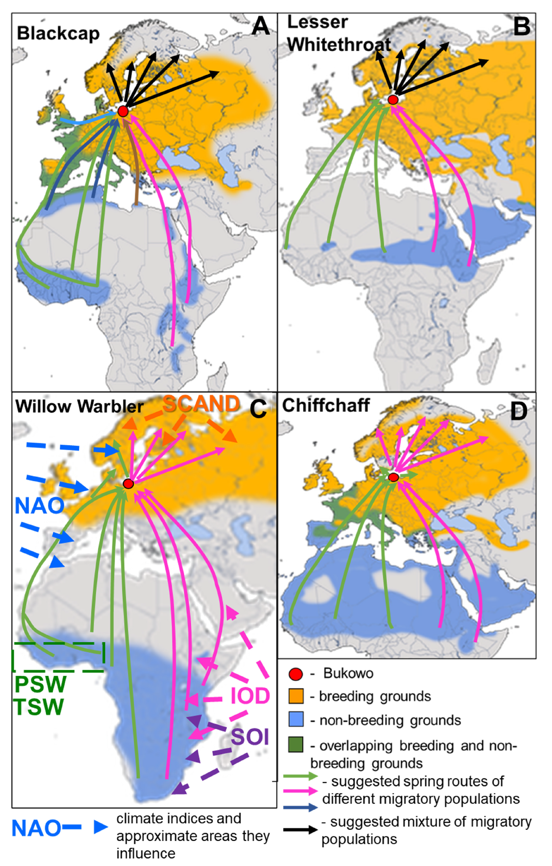
2.1. Study Species and Their Spring Migration Routes

We selected the four most numerous species of long-distance migrant passerines caught at the ringing station Bukowo (N Poland) during spring passage in 1982–2024 (Figure 1). These species are Willow Warbler, Chiffchaff, Blackcap, and Lesser Whitethroat; all of these are both common breeding birds across Europe and long-distance trans-Saharan migrants to and from wide-ranging non-breeding grounds in Africa and the Middle East (Figure 1). The Blackcap and Chiffchaff use wide wintering grounds that extend from western to eastern Africa, while the Willow Warbler uses all sub-Saharan areas of Africa extending to southeastern Africa (Figure 1). In the Lesser Whitethroat, the non-breeding range extends from a core in the Middle East and eastern Africa westwards to the central part of the Sahel (Figure 1). Some populations of the Blackcap and Chiffchaff breed and overwinter in southern and western Europe (Figure 1), but the populations breeding in northern Europe are entirely migratory [14].

2.1.1. Blackcap

The northern and northeastern breeding populations of Blackcap that migrate through the Baltic region including Bukowo, all belong to the nominate subspecies and are obligatory migrants, but their migratory patterns are rather complex [14]. The Blackcap populations which are the focus of this study include long-distance trans-Saharan migrants that use non-breeding grounds spanning west to east Africa, medium-distance migrants to and from northern Africa, and short-distance migrants that overwinter across the Mediterranean region of Europe and in the UK (Figure 1A) [10,11,12,38,39,41,46,47]. Thus, in spring, Bukowo supports migratory populations of the Blackcaps arriving from wintering quarters in West Africa (green arrows in Figure 1A) and from western part of the Mediterranean region of northern Africa and southern Europe (dark blue arrows) and. those from the UK (light blue arrows). In addition, Bukowo also supports those arriving from eastern Africa (pink arrows) or the eastern part of the Mediterranean region (brown arrow). Since about the 1980s, Blackcaps have shortened their migration distance, adjusting to climate change, and an increasingly greater proportion of Blackcaps overwinters north of the Sahara, across the whole Mediterranean region, and in the UK [46,47].

2.1.2. Lesser Whitethroat

All the Lesser Whitethroat populations breeding in northern and central Europe belong to the nominative subspecies and are obligatory migrants [14]. Lesser Whitethroats, which migrate in spring through the Baltic region, including Bukowo (Figure 1B), arrive mostly from the main part of the species’ non-breeding range, i.e., eastern Africa and the Middle East, along the Eastern Flyway (pink arrows in Figure 1B); this is well documented by ringing recoveries between these regions and northern Europe [10,11,12,44,48] and supported by the results of orientation experiments [40]. But the species’ non-breeding range extends west to the central part of the Sahel and patches of winter occurrence in west Africa, which is less known (Figure 1B). This information, as well as the several ringing recoveries of the area between central and northern Europe and Congo [10], indicate that Lesser Whitethroats probably also arrive in the Baltic region from central and western Africa (green arrows in Figure 1B) and breed locally or farther north and north-east.

2.1.3. Willow Warbler

In the Baltic region, two subspecies of Willow Warbler, P. trochilus trochilus and P. t. acredula, occur during spring migration [14]. The nominate subspecies arrives from wintering grounds in west and central Africa, then heads to the breeding grounds in southern Scandinavia and Poland (green arrows in Figure 1C). The subspecies acredula mostly uses the wintering grounds in central, eastern, and southern Africa, and breeds in eastern Poland, northern Sweden and Finland, and farther northeast (pink arrows at Figure 1C) [10,11,12,41,42,44,49,50]. The migratory divide between these subspecies at the breeding grounds runs across northeastern Poland and central Sweden [51,52,53,54], where the nominate subspecies arrives in April, about two weeks earlier than P. t. acredula [49]. Given this migration pattern, in spring, Bukowo supports a mixture of both subspecies of Willow Warblers arriving from most of the species’ wintering range, heading for their more northern and northeastern breeding grounds (Figure 1C), but with a prevalence of the nominate subspecies, which also breeds locally [7,8,9,45].

2.1.4. Chiffchaff

Two subspecies of Chiffchaff migrate through Bukowo and breed in the Baltic region and farther northwest: P. collybita collybita and P. c. abietinus [14,43,44,45]. The nominative subspecies breeds from southern Sweden, across central and eastern Europe to the Iberian Peninsula (Figure 1D). The northern populations of this subspecies, including those from the Baltic region, are mostly long-distance migrants, which winter in west Africa and the western part of the Mediterranean region, but also medium-distance migrants that winter closer to the breeding grounds at the Iberian Peninsula and in western Europe (green arrows in Figure 1D) [43,44,55]. P. c. abietinus breeds in northern and eastern Europe, from the northern part of Scandinavia to the Ural Mountains, and overwinters in northeastern and central Africa, as well as in the Middle East in the eastern Mediterranean region (pink arrows in Figure 1D) [43,44,45,55]. At Ottenby Bird Observatory, on the Baltic island of Öland (Sweden), during 1978–1984 birds of the abietinus subspecies were the first arriving Chiffchaffs, from the beginning of April until mid-June, while the collybita subspecies occurred only from the beginning of May onwards [56].

In these species, migratory populations arriving from different regions of wintering grounds along the western and eastern migration routes meet at stopover sites in central and northern Europe. Ringing recoveries of these four species indicate that our study site Bukowo (Figure 1) is a spring stopover location situated on the crossroads of the populations migrating to the north along the western, central and eastern flyways, between non-breeding quarters across Africa and breeding grounds in north-eastern Europe, including the Baltic region [10,11,12,41].

Considering that different migratory populations of each species are represented among spring migrants at Bukowo [7,8,9,41], we expected that their migration timing would be related to climatic conditions in different parts of their non-breeding grounds in Africa and the Mediterranean region, in a sequence reflecting the flyways used by populations subsequently arriving in our study site at the southern coast of the Baltic Sea (Figure 1).

2.2. Study Site and Methods of Fieldwork

To analyse patterns of spring migration of these four species, we used the daily totals of birds caught and ringed during spring migration in 1982–2024 at the ringing station Bukowo–Kopań (Figure 1), on the Baltic Sea coast (N Poland; 54°20′13″–54°27′11″ N, 16°14′36″–16°24′08″ E); we will call the station “Bukowo” further in the text. Birds were caught in mist nets daily in a monitoring manner, from dawn to dusk, during 26 March–15 May each year, which covers most of the spring migration period for the four studied species [8]. The station did not operate in spring 2011 and 2020 due to logistics and COVID-19 constraints. Birds were caught using 7 m long mist nets for passerines set up in the coastal forest and bushes across the narrow spits between the Baltic Sea and coastal lakes Bukowo and Kopań. The study site was moved between these two spits within 16 km of the coast in 2012 due to holiday housing development at Kopań location [8]. The number of mist nets was constant during each spring, but varied from 35 to 57 between different years. Capture and ringing followed the standardised monitoring protocols of the Operation Baltic project, which includes Bukowo station [57]. The details of catching locations and mist-netting habitats over the years have been described in our earlier paper [8].

In Blackcap, Lesser Whitethroat, and Chiffchaff, most individuals caught in spring are “young” (9–12 months old, or 2cy = in 2nd calendar year) or “adult” (older, 2cy+) according to EURING codes, but some individuals were difficult to age, and were thus recorded as “full-grown” (1cy+) [58,59]. In Willow Warblers, young and adult birds in spring cannot be distinguished by plumage, thus all individuals were aged as “full-grown” (1cy+) [58,59]. For consistency, we combined all age groups and analysed them jointly in the four species, because this was required for the Willow Warbler. With this approach, we assumed that individuals of any age in spring were heading for the breeding grounds to nest, as in our earlier studies [7,8,9].

2.3. Methods of Analysing Data on Migrant Birds

We analysed daily catching totals of the four study species caught at Bukowo each day during the annual study periods, including only the first capture of an individual in a season. For each species, we excluded from analyses the springs when fewer than 10 individuals of that species were caught. Thus, we analysed data for 38–41 spring seasons, depending on the species, collected during 43 years of the study (1982–2024) (Appendix A,

Table A1. The number of four migrants ringed and the number of used mist nets each spring in 1982–2024 at the Bukowo ringing station. N = numbers of birds of each species caught each spring (26 March–15 May), aged as “full grown”; N nets = number of 7 m passerine mist nets used each season, “–” = seasons excluded from analysis because fewer than 10 birds were caught; N years = numbers of years analysed for each species. The birds were caught in two coastal locations 16 km apart: Kopań (54°27′11″ N, 16°24′08″ E) and Bukowo (54°20′13″ N, 16°14′36″ E).

Year	Location	N Chiffchaff	N Willow Warbler	N Lesser Whitethroat	N Blackcap	N Nets
1982	Kopań	90	1016	123	88	57
1983	Kopań	100	498	186	80	57
1984	Kopań	52	180	48	22	42
1985	Kopań	39	189	42	13	51
1986	Kopań	29	62	12	24	50
1987	Kopań	42	76	–	–	45
1988	Kopań	28	64	25	35	45
1989	Kopań	48	84	40	11	45
1990	Kopań	31	34	20	–	45
1991	Kopań	77	52	50	28	45
1992	Kopań	18	31	31	16	37
1993	Kopań	73	–	–	–	–
1994	Kopań	58	71	85	60	47
1995	Kopań	59	79	99	35	47
1996	Kopań	51	108	88	64	47
1997	Kopań	63	161	80	110	47
1998	Kopań	92	80	112	117	47
1999	Kopań	70	133	80	133	47
2000	Kopań	85	72	89	120	47
2001	Kopań	91	95	147	180	57
2002	Kopań	61	92	99	136	47
2003	Kopań	91	58	67	175	46
2004	Kopań	92	99	108	163	47
2005	Kopań	132	177	228	280	47
2006	Kopań	108	107	126	297	47
2007	Kopań	87	147	183	212	54
2008	Kopań	129	115	182	150	50
2009	Kopań	131	107	155	257	46
2010	Kopań	148	85	163	288	35
2011	–	–	–	–	–	–
2012	Bukowo	89	138	63	334	56
2013	Bukowo	88	85	115	391	51
2014	Bukowo	120	71	103	224	48
2015	Bukowo	75	42	62	198	51
2016	Bukowo	87	72	54	374	52
2017	Bukowo	47	78	71	186	52
2018	Bukowo	110	59	89	279	52
2019	Bukowo	138	73	88	295	52
2020	–	–	–	–	–	–
2021	Bukowo	79	68	87	370	46
2022	Bukowo	154	118	130	326	57
2023	Bukowo	192	88	85	335	47
2024	Bukowo	337	58	19	434	47
	N years	41	40	39	38

). For each species, we calculated the daily catch totals as a daily percentage in relation to the total number of this species caught that spring. These daily percentages were summarised for each spring to produce annual cumulative arrival curves for each species (red line in Figure 2 is an example for 1996). The values from these cumulative curves were averaged for each day between 26 March and 15 May across the studied years to derive the multi-year (1982–2024) average cumulative curve of spring arrival for each species (red line in Figure 2). Because these calculations were based on daily percentages, the fact that the number of mist nets in each year was not identical has no impact on the results. In the next step, for each species, we derived the Annual Anomaly (AA) of spring passage in each year, as in earlier papers [7,8,9,60,61]. AA for each spring was calculated as the sum of daily departures of the cumulative arrival curve for that spring from the multi-year average curve of spring passage, across the whole spring season (26 March–15 May) in question (the grey area in Figure 2 is an example for 1996) A negative value of AA for a spring indicated that spring passage was earlier than average, and a positive AA, analogously, indicated spring passage was later than average [7]. In this way, for each species, we obtained a time series of AAs of passage, which indicated how early or late the spring passage was in each year, in relation to the average spring passage in 1982–2024, which was used as a baseline.

Next, for each species, using its multi-year cumulative curve (red line in Figure 2), we found the dates when each third of birds had, on average, passed each spring, i.e., 0–33%, 34–66%, 67–100% (

Table 1. Division of the Annual Anomaly (AA) into three main periods (MP1–MP3) and nine sub-periods (SP1–SP9) of spring, used as response variables in modelling relationships between timing of passage within these periods of spring and selected climate variables, at Bukowo (N Poland) over 1982–2024. Percentiles = the ranges of percentiles used to derive the dates for the main periods (MP1–MP3) and sub-periods (SP1–SP9) of AA, from the many-year average curve for each species.

Symbol	Percentiles	Dates for Each Period by Species
		Chiffchaff	Willow Warbler	Blackcap	Lesser Whitethroat
AA	0–100%	26 March–15 May 1
MP1	0–33%	26 Mar–12 Apr	1–26 Apr	1–30 Apr	1–30 Apr
MP2	34–66%	13–23 Apr	27 Apr–5 May	27 Apr–5 May	1–8 May
MP3	67–100%	24 Apr–15 May	6–15 May	6–15 May	9–15 May
SP1	0–20%	26 Mar–7 Apr	1–22 Apr	1–23 Apr	1–24 Apr
SP2	11–30%	4–11 Apr	18–25 Apr	20–26 Apr	25–30 Apr
SP3	21–40%	8–14 Apr	24–28 Apr	24–28 Apr	28 Apr–2 May
SP4	31–50%	12–17 Apr	26 Apr–1 May	27–30 Apr	1–4 May
SP5	41–60%	15–20 Apr	29 Apr–3 May	29 Apr–2 May	3–6 May
SP6	51–70%	18–24 Apr	2–5 May	1–6 May	5–9 May
SP7	61–80%	21–28 Apr	4–7 May	3–8 May	7–10 May
SP8	71–90%	25 Apr–4 May	6–11 May	7–10 May	10–13 May
SP9	81–100%	29 Apr–15 May	9–15 May	11–15 May	11–15 May

¹ The overall AA was calculated for the whole spring season (26 March–15 May) for all species. The dates of the subsequent main periods (MP) and sub-periods (SP) differ between the species, according to the species-specific phenology of spring passage.

; Figure 2).

Using these species-specific dates, we divided the Annual Anomaly for each spring into three non-overlapping main periods (MP1–MP3) (Table 1; Figure 2). For each species, these three anomalies (for periods MP1–MP3 of spring) indicated whether the timing of passage of the first (MP1), middle (MP2), and the last third of migrants (MP3), was early or late that year, in relation to the multi-year average migration curve in that third of passage (Table 1; Figure 2). In this way, for each species, we derived three time series that reflected year-to-year changes in the timing of passage of the first, middle, and last third of spring migrants over the 1982–2024 study period.

For each species, to further analyse the expected changes in the effects of the climate variables across spring, we divided AA in each year into nine overlapping sub-periods of the AA (SP1–SP9), according to dates which spanned 20% intervals of the multi-year cumulative curve (0–20%, 11–30%, 21–40%, 31–50%,…, 81–100%; Table 1, Figure 2). This way we obtained nine time series, which reflected annual changes of passage in these nine overlapping parts of spring across 1982–2024 in each species. The methods we applied are the same as in earlier papers, described there in more detail.

2.4. Climate Indices Selected for the Study

To identify the effects of the climate factors on the timing of spring migration of the four species at Bukowo station, we used 14 climate variables (

Table 2. Climate indices used as explanatory variables in modelling the timing of spring passage (26 March–15 May) of long-distance migrants at Bukowo (N Poland) over 1982–2024. The climate indices were downloaded from the listed sources. All databases were last accessed on 23 June 2025.

No	Symbol of Variable 1	Climate Index	Region Under Climatic Influence	Key References	Source
1	SCA APR–MAY	Scandinavian Pattern Index	Scandinavia, western and central Russia	[62,63]	ftp://ftp.cpc.ncep.noaa.gov/wd52dg/data/indices/scand_index.tim (accessed on 23 June 2025)
2	SCA MAY–JUL_1Y
3	TBK APR–MAY	Mean local temperature	Baltic coast near Bukowo (54–55° N, 16° E–18° E)	[64]	http://climexp.knmi.nl/select.cgi?era5_t2m_daily (accessed on 23 June 2025)
4	PBK APR–MAY	Mean local precipitation			https://climexp.knmi.nl/select.cgi?gpcc (accessed on 23 June 2025)
5	NAO APR–MAY	North Atlantic Oscillation Index	Northwestern and Central Europe, Western Mediterranean area, Northwestern Africa	[35,65,66,67,68]	https://www.cpc.ncep.noaa.gov/products/precip/CWlink/pna/norm.nao.monthly.b5001.current.ascii.table (accessed on 23 June 2025)
6	NAO AUG–OCT_1Y
7	NAO NOV–MAR
8	TSW AUG–OCT_1Y	Temperature in the Western Sahel	Western Sahel (15–20° N, 20° W–10° E)	[69,70]	http://climexp.knmi.nl/select.cgi?era5_t2m_daily (accessed on 23 June 2025)
9	TSW NOV–MAR
10	PSW AUG–OCT_1Y	Precipitation for the Western Sahel			https://climexp.knmi.nl/select.cgi?gpcc (accessed on 23 June 2025)
11	PSW NOV–MAR
12	IOD AUG–OCT_1Y	Indian Ocean Dipole	East Africa, Middle East	[71,72,73,74]	http://climexp.knmi.nl/getindices.cgi?WMO=UKMOData/hadisst1_dmi&STATION=DMI_HadISST1&TYPE=i&id=someone@somewhere (accessed on 23 June 2025)
13	IOD NOV–MAR
14	SOI NOV–MAR	Southern Oscillation Index	East Africa, southeastern Africa	[75]	http://climexp.knmi.nl/getindices.cgi?WMO=CRUData/soi&STATION=SOI&TYPE=i&id=someone@somewhere (accessed on 23 June 2025)

¹ Abbreviations include the months for which the mean values of each climate index were averaged; _1Y indicate the months of the year prior to the year of the analysed spring migration.

), including large-scale climatic indices; temperature and precipitation for the Western Sahel; and local values of temperature and precipitation for the coastal area, including Bukowo.

The large-scale climate indices we used (SCA, NAO, IOD, SOI; Table 2) are derived by meteorologists as the differences in the normalised sea level pressures between two selected weather stations, which reflect atmospheric oscillation patterns [76]. These oscillations shape the temperature, precipitation, wind direction, and cloudiness at a much larger geographical scale in Europe and Africa than just the areas between the compared locations (Table 2). We used these climate indices, which reflect all weather features at once, as proxies for environmental conditions over wide areas; other studies have focused on the influence of climate on bird migrations [8,16,21,34,35,36,61,77]. We use such large-scale climate patterns for analyses as we have only a general knowledge of areas visited by small migrants during a year. This is based on the limited number of ringing recoveries available [10,41], as most tracking devices are still too heavy for small birds [78]. We downloaded these large-scale indices from the listed online weather services (Table 2) as monthly values, which we then averaged for selected months.

For the Western Sahel, in the absence of any convenient climate index for that region, we downloaded temperatures and rainfall data for the same area of western Africa (Figure 1A, Table 2) as in our earlier studies [7,8,9] and in the earlier papers which used the Sahel Precipitation Index (SPI) [13,18,79], to enable comparisons. To analyse the effects of local weather on migrants arriving at Bukowo, we also used temperature and precipitation for the region of the southern coast of the Baltic Sea, including both Bukowo and Kopań ringing locations (Table 2). We downloaded daily data on mean temperature and total precipitation, averaged based on weather models and readings from the weather stations located within the selected range of coordinates (Table 1), using the Climate Explorer by the World Meteorological Organisation (https://climexp.knmi.nl/ (accessed on 23 June 2025)) and based on data from the European Climate Assessment and Dataset (http://www.ecad.eu (accessed on 23 June 2025)). We derived monthly means of temperature and precipitation, then averaged them for selected months.

We used a similar set of climate variables as in our earlier studies focused on six long-distance migrants, including the four species we analyse here [8]. We averaged these climate indices for the months corresponding to the general life stages of these long-distance migrants during the 12 months preceding the spring migration: (1) “breeding period” = May–July of the previous year, (2) “autumn migration” = August–October of the previous year; (3) “wintering” = November of the previous year–March of the spring migration year; (4) “spring migration” = April–May. The ranges of these four species are mostly in the northern hemisphere, and we use northern seasons. For analyses, we selected only the climate variables for the periods when the migrants visit areas where these factors operate (Table 2), as we did in earlier papers [7,8,9].

In this way, we initially chose 15 climate variables, but SOI in autumn (August–October) and winter (November–March) were strongly correlated (Pearson’s correlation coefficient r = 0.85), which might cause bias in the results of our multiple regression models [80]. Thus, we excluded SOI in August–October from the models as it had rarely been an important explanatory variable in our prior analyses, but we included SOI in November–March, which affected the spring passage of Willow Warbler in our earlier analyses [9]. In this way, we selected 14 climate variables for analysis, which were all correlated at |r| < 0.7 (

Table A2. Pearson’s correlation coefficients of climate indices in 1981–2024 we used in multiple regression models. Abbreviations of the climate variables as in Table 2; “_1y” = climate indices from the year preceding the spring being analysed. Significant correlations after Benjamini–Hochberg correction for multiple comparisons with an accepted 5% level of false positives marked in red font.

	IOD NOV_ MAR	NAO APR_MAY	NAO AUG_ OCT_1Y	NAO NOV_ MAR	PBK APR_ MAY	PSW AUG_ OCT_1Y	PSW NOV_ MAR	SCA MAY_ JUL_1Y	SOI NOV_ MAR	TBK APR_ MAY	TSW AUG_ OCT_1Y	TSW NOV_ MAR
IOD_AUG_OCT_1Y	0.60	−0.19	−0.20	0.25	−0.04	0.15	−0.15	−0.03	−0.39	0.11	0.14	0.03
IOD_NOV_MAR		−0.25	−0.17	−0.03	−0.32	0.18	−0.29	0.22	−0.10	0.19	0.14	0.22
NAO_APR_MAY			−0.16	0.06	−0.20	0.07	0.10	−0.01	0.07	−0.07	−0.13	−0.19
NAO_AUG_OCT_1Y				−0.09	0.24	−0.09	0.23	0.16	−0.15	0.00	−0.27	−0.21
NAO_NOV_MAR					−0.23	0.15	−0.20	−0.06	−0.15	0.53	−0.17	−0.43
PBK_APR_MAY						−0.18	0.04	−0.11	−0.29	−0.40	−0.10	−0.25
PSW_AUG_OCT_1Y							−0.16	0.01	0.26	0.26	−0.43	−0.02
PSW_NOV_MAR								−0.14	−0.23	−0.18	−0.04	0.06
SCA_MAY_JUL_1Y									0.15	0.12	−0.23	−0.29
SOI_NOV_MAR										0.06	0.00	0.13
TBK_APR_MAY											0.10	0.05
TSW_AUG_OCT_1Y												0.67

), indicating that any influence of their multicollinearity on the models’ results should be small [80].

Some of the climate indices we analysed show multi-year trends, e.g., temperatures and precipitation in the Sahel, and IOD, in autumn or winter, but some others, e.g., NAO or SCA for most seasons, do not show any trends [8]. More information on these climate indices and an overview of their effects on long-distance migrants within the Euro-African migration system have been provided in [8].

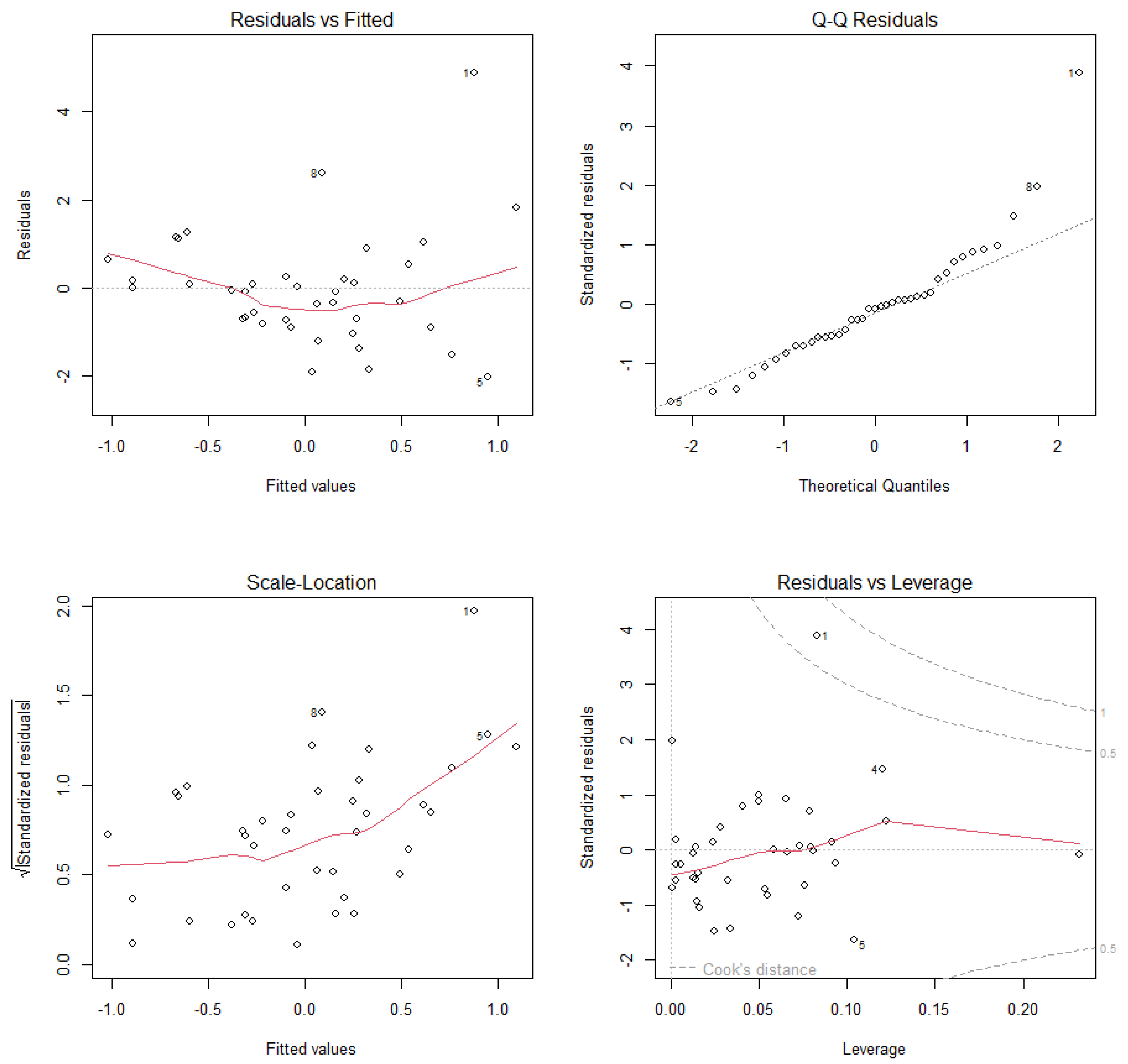
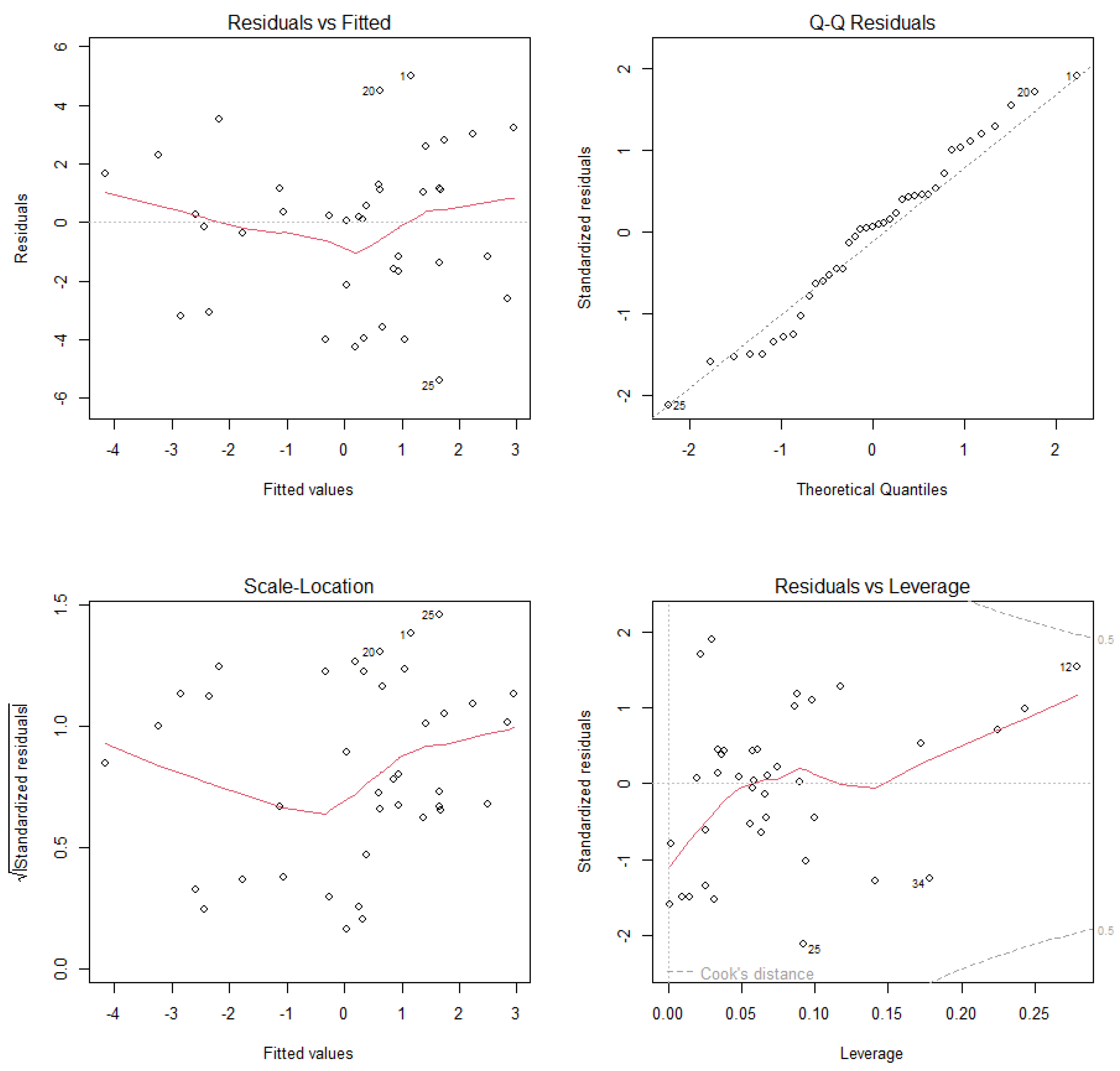
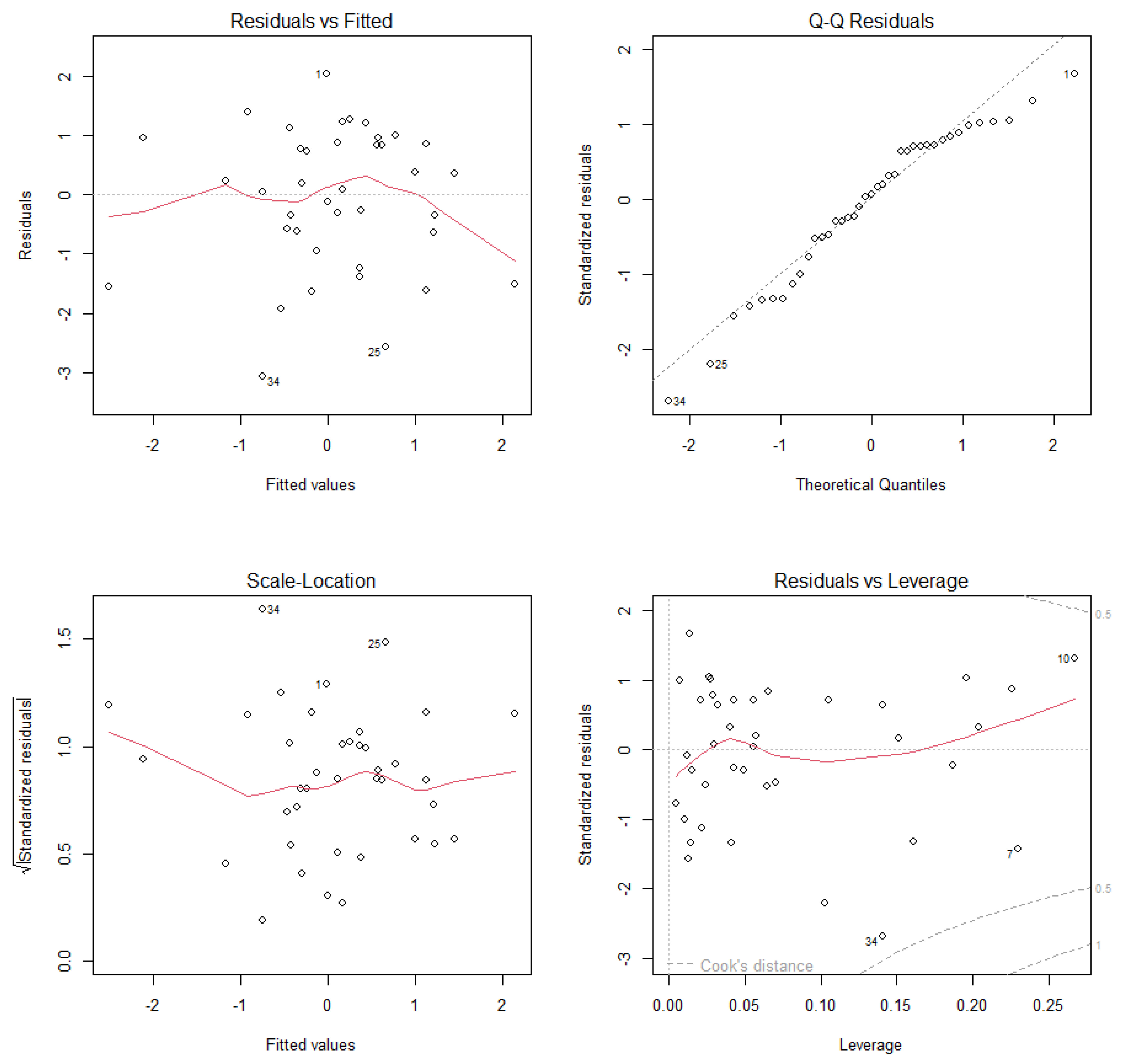
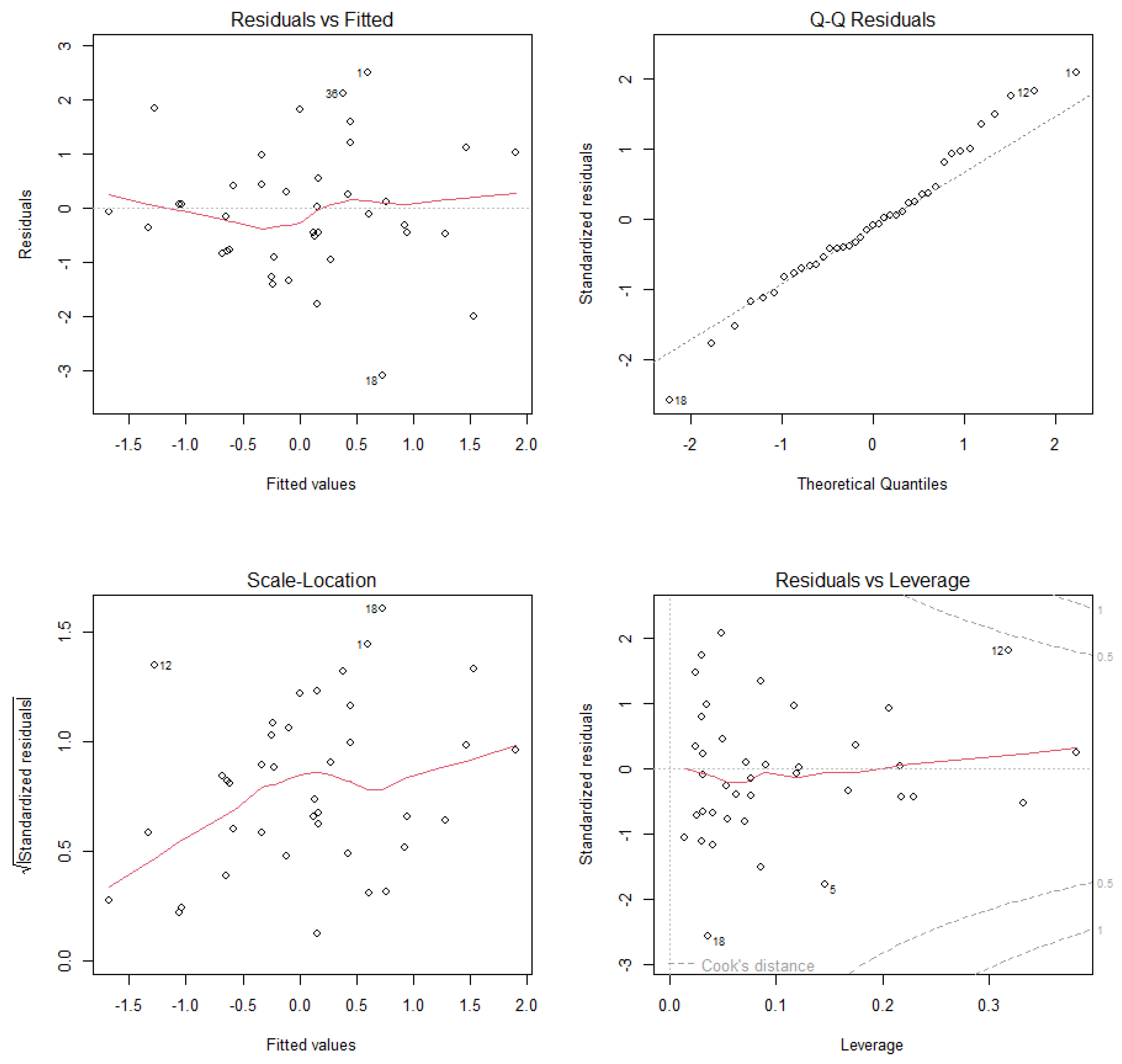
2.5. Methods of Statistical Analysis

To check if the timing of spring migration of each species showed trends over the period 1982–2024, we analysed time series of the overall annual anomalies (AA) using linear regression against year. Next, for each species, we used four time series (AA, MP1–MP3) over 1982–2024 as response variables in multiple regression models, with the 14 climate indices (Table 1) as explanatory variables. Explanatory variables were at different scales; we therefore standardised all of them (Table 2) so that they had a mean of 0 and a standard deviation of 1, making their effects obtained from the multiple regression comparable. All response variables (Table 1) were on the same scale and measured in days; therefore, we did not standardise these variables to facilitate interpretation of the results. To monitor for any bias by multicollinearity, we checked Variance Inflation Factors (VIF) in multiple regression models; if VIF < 10, the bias is negligible [80]. For each species, we first ran four multiple regression models, with AA and MP1–MP3 as response variables (Table 1) and all the climate variables (Table 2) as explanatory variables. We used the “all subsets regression” procedure and selected the best model using the Akaike Information Criteria corrected for small sample size (AICc), applying the package “MuMIn 1.48.11” [81]. Using 14 explanatory variables in models with 38–41 data points (years), we risked model overfitting. To assess if our final best models were overfitted, we cross-validated the best models in each multiple regression analysis using the three methods recommended by [82]: (1) drawing model diagnostic plots, which identify outliers and indicate influential data points using Cook’s distance [83]; (2) calculating the ratio of the multiple coefficient of determination (R²) to the adjusted coefficient of determination (AdjR²), the closer the ratio is to 1, the better is the fit of model to the data; (3) comparing the adjusted coefficient of determination (AdjR²) and the predictive coefficient of determination (predR²). The predictive R² is calculated by removing a data point from the dataset, calculating the regression again, assessing how well the model predicts the missing observation, and repeating this procedure for each data point. If AdjR² is close to the predR² (the difference between these two values is close to 0), this means that the tested model predicts the new observations as well as it fits the original dataset, thus the model is stable and not overfitted. For these methods, we used the following procedures: for method (1), we used an R script according to [83]; for methods (2) and (3), we used an R script by Antonello Pareto [84]. If all these methods indicated that the best model was not overfitted, we used this model in further steps.

For each climate variable selected in the best model for AA and MP1–MP3, we calculated the partial correlation coefficient (pR) using the package “ppcor 1.1” [81]. This coefficient (pR) reflects the correlation between the response variable and each climate index while removing the effects of the remaining climate factors from the models. We plotted pR coefficients as bars to visualise the results of the best models and compare the effects of each climate variable, as in our earlier studies [7,8,9,61,77].

Six to nine climate variables, depending on the species, were selected in the best-fitted models for AA and MP1, MP2 and MP3, and also had the greatest contributions in the sets of top models (ΔAICc < 2). For each species, we selected these variables as the species-specific set of climate factors which showed any influence on the timing of spring migration at Bukowo. We further investigated the pattern of change through the spring arrival period of the effects of these climate factors. We did this by fitting the explanatory variables to the annual anomalies for each of the nine overlapping sub-periods (SP1–SP9) of spring passage (Table 1, Figure 2). We used these as consecutive response variables, in multiple regression models, separately for each species.

In each species, the sub-periods with uneven numbers (SP1, SP3, SP5, SP7, SP9) did not overlap (Table 1), and thus, the results from models for these periods can be compared as a series of multiple regression models. Analogously, the sub-periods with even numbers (SP2, SP4, SP6, SP8) also do not overlap, and thus, the results for these sub-periods can also be directly compared. But the nine “uneven” and “even” sub-periods of spring (SP1-SP9) overlap (Table 1). Thus, the relationships with the climate variables for all these periods cannot be interpreted as independent, but rather as a visual exploratory analysis of data using a “moving window” approach, trying to reveal the changing relationship between the climate variables and the successive “sections” of the annual anomaly during the spring passage [85]. For each species, we plotted the partial correlation coefficient (pR) from the models for SP1–SP9 to visualise the changes in the effect of each climate factor on the timing of subsequent cohorts of migrants arriving in these sub-periods, as in our earlier study on Willow Warbler [9]. All our results are based on the correlation analyses using multiple regression models. Thus, we do not know whether the relationships we revealed reflect the actual cause–effect influence of a climate factor on timing of migrants, or a common pattern which has been reflected by their correlation. Hence, any causal interpretation of these results should be treated with caution [86]. All statistical analyses were conducted in R v. 4.3.3 [87].

3. Results

3.1. Multi-Year Trends in the Spring Passage Timing at the Baltic Sea Coast for the Four Study Species

During the studied 43 years, the overall timing of the spring passage at Bukowo, reflected by the Annual Anomaly (AA), shifted over 1982–2024 to be significantly earlier for the Chiffchaff (Figure 3A), Willow Warbler (Figure 3B), and the Blackcap (Figure 3C), on average by 5.8, 4.2, and 4.5 days, respectively. For the Lesser Whitethroat, we found no long-term linear trend in migration timing (Figure 3D).

The linear regressions, even those that were significant, explained small percentages (2% to 13%) of the variation in the timing of passage during spring (AA) (Figure 3). Thus, we investigated the extent to which climate factors played roles in the annual variation in the phenology of the four species.

3.2. Effects of Climate Factors on the Entire Spring Passage (AA) and Its Three Main Periods (MP1–MP3) in the Four Studied Species

The best models for the four species explained 10.2–59.4% of their variation in migration timing, measured by AA, and selected 1–7 climate variables (Figure 4;

Table 3. Effects of the climate variables selected in the best models on the timing of the overall spring passage (AA) and its three main periods (MP1–MP3) in 1982–2024 for the Chiffchaff Phylloscopus collybita caught at Bukowo, N Poland. Estimate = coefficients from multiple regression, SE = standard error of the estimates; t, p = t-test and significance of each estimate. VIF = variance inflation factor, pR = Pearson’s partial correlation coefficients (presented as bars in Figure 4). AdjR² = adjusted coefficient of determination, predR² = predictive coefficient of determination, if AdjR² − predR² is close to 0 the model is stable and not overfitted. Model diagnostics plots are presented in Figure A1, Figure A2, Figure A3 and Figure A4, and the full model is presented in Table A4 in Appendix A.

Response Variable /Climate Variable	Estimate	SE	t	p	VIF	pR
AA Best model: F5,36 = 4.79, AdjR2 = 31.6%, AdjR2/R2 = 0.79, AdjR2 − predR2 = 0.15
IOD_AUG_OCT_1Y	–2.66	0.81	–3.29	0.0023	1.57	–0.48
IOD_NOV_MAR	1.28	0.80	1.61	0.1163	1.76	0.26
NAO_AUG_OCT_1Y	–1.26	0.62	–2.02	0.0508	1.10	–0.32
PBK_APR_MAY	1.91	0.64	2.97	0.0052	1.22	0.45
TSW_NOV_MAR	–1.48	0.64	–2.33	0.0256	1.12	–0.36
MP1 Best model: F4,37 = 4.44, AdjR2 = 25.1%, AdjR2/R2 = 0.78, AdjR2 − predR2 = 0.08
NAO_AUG_OCT_1Y	–0.57	0.26	–2.23	0.0316	1.13	–0.14
PBK_APR_MAY	0.46	0.25	1.89	0.0671	1.08	0.24
PSW_AUG_OCT_1Y	–0.53	0.30	–1.78	0.0841	1.40	–0.19
TSW_AUG_OCT_1Y	–0.97	0.29	–3.40	0.0016	1.48	–0.38
MP2 Best model: F6,35 = 4.86, AdjR2 = 36.1%, AdjR2/R2 = 0.79, AdjR2 − predR2 = 0.16
IOD_AUG_OCT_1Y	–0.40	0.24	–1.64	0.1101	1.12	–0.27
NAO_APR_MAY	–0.49	0.22	–2.21	0.0341	1.12	–0.35
NAO_AUG_OCT_1Y	–0.57	0.23	–2.48	0.0179	1.20	–0.39
PBK_APR_MAY	0.51	0.22	2.34	0.0252	1.12	0.37
PSW_AUG_OCT_1Y	–0.57	0.27	–2.14	0.0397	1.50	–0.34
TSW_AUG_OCT_1Y	–0.86	0.26	–3.33	0.0021	1.61	–0.49
MP3 Best model: F3,38 = 4.12, AdjR2 = 18.6%, AdjR2/R2 = 0.76, AdjR2 − predR2 = 0.10
IOD_AUG_OCT_1Y	–1.16	0.38	–3.05	0.0041	1.49	–0.44
IOD_NOV_MAR	0.61	0.37	1.64	0.1084	1.67	0.26
PBK_APR_MAY	0.65	0.30	2.15	0.0377	1.16	0.33

,

Table 4. Effects of the climate variables selected in the best models on the timing of the overall spring passage (AA) and its three main periods (MP1–MP3) in 1982–2024 for the Willow Warbler Phylloscopus trochilus caught at Bukowo, N Poland. Symbols as in Table 3. Model diagnostics plots are presented in Figure A5, Figure A6, Figure A7 and Figure A8, and the full model is presented in Table A5 in Appendix A.

Response Variable /Climate Variable	Estimate	SE	t	p	VIF	pR
AA Best model: F7,33 = 6.80, AdjR2 = 50.4%, AdjR2/R2 = 0.85, AdjR2 − predR2 = 0.09
IOD_AUG_OCT_1Y	–1.67	0.51	–3.27	0.0025	1.49	–0.50
IOD_NOV_MAR	1.34	0.55	2.47	0.0190	2.05	0.40
NAO_APR_MAY	–1.16	0.41	–2.83	0.0079	1.19	–0.44
PBK_APR_MAY	0.78	0.46	1.68	0.1030	1.48	0.29
PSW_AUG_OCT_1Y	–2.02	0.55	–3.67	0.0009	1.93	–0.54
SCA_MAY_JUL_1Y	–0.96	0.41	–2.33	0.0259	1.28	–0.38
TSW_AUG_OCT_1Y	–1.82	0.54	–3.37	0.0019	2.08	–0.51
MP1 Best model: F6,34 = 8.78, AdjR2 = 53.9%, AdjR2/R2 = 0.89, AdjR2 − predR2 = 0.12
IOD_AUG_OCT_1Y	–0.73	0.22	–3.28	0.0024	1.34	–0.49
NAO_APR_MAY	–0.64	0.18	–3.62	0.0009	1.04	–0.53
PSW_AUG_OCT_1Y	–0.80	0.24	–3.33	0.0021	1.76	–0.50
SCA_MAY_JUL_1Y	–0.33	0.18	–1.84	0.0741	1.14	–0.30
SOI_NOV_MAR	–0.57	0.21	–2.73	0.0099	1.34	–0.43
TSW_AUG_OCT_1Y	–0.86	0.23	–3.77	0.0006	1.77	–0.54
MP2 Best model: F6,34 = 6.30, AdjR2 = 44.3%, AdjR2/R2 = 0.84, AdjR2 − predR2 = 0.09
IOD_AUG_OCT_1Y	–0.66	0.24	–2.77	0.0089	–0.43	1.45
IOD_NOV_MAR	0.49	0.24	2.00	0.0534	0.33	1.82
NAO_APR_MAY	–0.65	0.18	–3.54	0.0012	–0.52	1.06
PSW_AUG_OCT_1Y	–0.98	0.25	–3.95	0.0004	–0.56	1.76
SCA_MAY_JUL_1Y	–0.43	0.19	–2.18	0.0360	–0.35	1.27
TSW_AUG_OCT_1Y	–0.88	0.24	–3.63	0.0009	–0.53	1.87
MP3 Best model: F1,39 = 5.55, AdjR2 = 10.2%, AdjR2/R2 = 0.82, AdjR2 − predR2 = 0.01
NAO_NOV_MAR	–0.24	0.10	–2.36	0.0236	–	–0.24

,

Table 5. Effects of the climate variables selected in the best models on the timing of the overall spring passage (AA) and its three main periods (MP1–MP3) in 1982–2024 for the Blackcap Sylvia atricapilla caught at Bukowo, N Poland. Symbols as in Table 3. Model diagnostics plots are presented in Figure A9, Figure A10, Figure A11 and Figure A12, and the full model is presented in Table A6 in Appendix A.

Response Variable /Climate Variable	Estimate	SE	t	p	VIF	pR
AA Best model: F3,36 = 5.07, AdjR2 = 23.9%, AdjR2/R2 = 0.80, AdjR2 − predR2 = 0.04
IOD_AUG_OCT_1Y	–1.04	0.56	–1.86	0.1189	1.02	0.30
NAO_APR_MAY	–1.03	0.55	–1.87	0.0113	1.09	–0.30
PBK_APR_MAY	1.20	0.51	2.35	0.0160	1.08	0.36
MP1 Best model: F2,37 = 10.17, AdjR2 = 32.0%, AdjR2/R2 = 0.90, AdjR2 − predR2 = 0.04
PBK_APR_MAY	0.72	0.20	3.68	0.0007	1.02	0.52
PSW_AUG_OCT_1Y	–0.43	0.21	–2.08	0.0448	1.02	–0.33
MP2 Best model: F2,37 = 5.81, AdjR2 = 19.8%, AdjR2/R2 = 0.83, AdjR2 − predR2 = 0.02
NAO_APR_MAY	–0.36	0.20	–1.78	0.0829	1.07	–0.28
PBK_APR_MAY	0.45	0.19	2.36	0.0234	1.07	0.36
MP3 Best model: F2,37 = 2.99, AdjR2 = 9.2%, AdjR2/R2 = 0.67, AdjR2 − predR2 = 0.07
NAO_NOV_MAR	–0.49	0.24	–2.04	0.0487	1.25	–0.32
TSW_NOV_MAR	–0.51	0.24	–2.11	0.0413	1.25	–0.33

and

Table 6. Effects of the climate variables selected in the best models on the timing of the overall spring passage (AA) and its three main periods (MP1–MP3) in 1982–2024 for the Lesser Whitethroat Curruca curruca caught at Bukowo, N Poland. Symbols as in Table 3. Model diagnostics plots are presented in Figure A13, Figure A14, Figure A15 and Figure A16, and the full model is presented in Table A7 in Appendix A.

Response Variable /Climate Variable	Estimate	SE	t	p	VIF	pR
AA Best model: F3,36 = 5.48, AdjR2 = 25.6%, AdjR2/R2 = 0.85, AdjR2 − predR2 = 0.07
IOD_AUG_OCT_1Y	–0.77	0.48	–1.60	0.1189	1.03	–0.26
NAO_APR_MAY	–1.21	0.45	–2.67	0.0113	1.02	–0.41
PSW_AUG_OCT_1Y	–1.15	0.46	–2.53	0.0160	1.01	–0.39
MP1 Best model: F3,36 = 6.84, AdjR2 = 30.1%, AdjR2/R2 = 0.89, AdjR2 − predR2 = 0.09
NAO_APR_MAY	–0.58	0.21	–2.78	0.0087	1.00	–0.42
PSW_AUG_OCT_1Y	–0.63	0.21	–3.01	0.0047	1.00	–0.45
SCA_MAY_JUL_1Y	–0.36	0.19	–1.88	0.0681	1.00	–0.30
MP2 Best model: F4,35 = 4.15, AdjR2 = 24.4%, AdjR2/R2 = 0.84, AdjR2 − predR2 = 0.07
IOD_AUG_OCT_1Y	–0.71	0.26	–2.67	0.1189	1.44	–0.41
IOD_NOV_MAR	0.73	0.26	2.83	0.0113	1.68	0.43
PBK_APR_MAY	0.48	0.22	2.16	0.0160	1.22	0.35
PSW_AUG_OCT_1Y	–0.43	0.21	–2.01	0.1189	1.06	–0.32
MP3 Best model: F1,38 = 2.51, AdjR2 = 3.7%, AdjR2/R2 = 0.82, AdjR2 − predR2 = 0.01
PSW_AUG_OCT_1Y	–0.14	0.09	–1.58	0.1217	–	–0.14

). For all best models, an inspection of the residuals (Figure A1, Figure A2, Figure A3, Figure A4, Figure A5, Figure A6, Figure A7, Figure A8, Figure A9, Figure A10, Figure A11, Figure A12, Figure A13, Figure A14, Figure A15 and Figure A16) showed that they met the assumptions of multiple linear regression [83]. The differences between adjusted and predictive coefficients of determination were in all models AdjR² − predR² $\le$ 0.10, indicating that the models were not overfitted (Table 3, Table 4, Table 5 and Table 6). Even in the few models with the slightly higher value of AdjR² − predR² $>$ 0.10, the ratios AdjR²/R² were $\ge$0.76, indicating that these models provide a satisfactory fit to the data. In all the best models (Table 3, Table 4, Table 5 and Table 6), as well as in full models (

Table A4. Full model of relationships between all 14 climate variables and Annual Anomaly of the timing of spring migration for the Chiffchaff Phylloscopus collybita caught at Bukowo, Poland, in 1982–2024. Estimate = coefficients from multiple regression, SE = standard error of the estimates; t, p = t-test and significance of each estimate. VIF = variance inflation factor, pR = Pearson’s partial correlation coefficient. AdjR² = adjusted coefficient of determination.

Response Variable /Climate Variable	Estimate	SE	t	p	VIF	pR
AA Full model: F13,28 = 1.99, AdjR2 = 24.0%
TBK_APR_MAY	−0.12	0.13	−0.91	0.3683	1.05	0.03
PBK_APR_MAY	1.71	0.90	1.90	0.0681	2.15	0.11
NAO_APR_MAY	−0.73	0.73	−1.00	0.3277	1.35	0.03
NAO_NOV_MAR	0.22	0.97	0.23	0.8219	2.33	0.00
IOD_NOV_MAR	1.60	1.06	1.51	0.1425	2.80	0.08
SOI_NOV_MAR	0.23	0.84	0.27	0.7858	1.69	0.00
NAO_AUG_OCT_1Y	−1.42	0.72	−1.97	0.0588	1.32	0.12
IOD_AUG_OCT_1Y	−2.51	1.00	−2.52	0.0179	2.14	0.18
SCA_MAY_JUL_1Y	−0.43	0.76	−0.57	0.5758	1.56	0.01
PSW_NOV_MAR	0.28	0.73	0.39	0.7023	1.44	0.01
PSW_AUG_OCT_1Y	−1.32	0.95	−1.39	0.1765	2.15	0.06
TSW_NOV_MAR	−1.33	1.29	−1.03	0.3119	4.13	0.04
TSW_AUG_OCT_1Y	−1.13	1.16	−0.97	0.3384	3.63	0.03
TBK_APR_MAY	−0.12	0.13	−0.91	0.3683	1.05	0.03
MP1 Full model: F13,28 = 1.45, AdjR2 = 12.0%
TBK_APR_MAY	−0.04	0.06	−0.77	0.4471	1.05	0.02
PBK_APR_MAY	0.62	0.38	1.66	0.1090	2.15	0.09
NAO_APR_MAY	0.07	0.31	0.23	0.8233	1.35	0.00
NAO_NOV_MAR	0.22	0.41	0.54	0.5964	2.33	0.01
IOD_NOV_MAR	0.28	0.44	0.63	0.5337	2.80	0.01
SOI_NOV_MAR	0.19	0.35	0.54	0.5908	1.69	0.01
NAO_AUG_OCT_1Y	−0.60	0.30	−2.01	0.0540	1.32	0.13
IOD_AUG_OCT_1Y	−0.44	0.42	−1.05	0.3021	2.14	0.04
SCA_MAY_JUL_1Y	−0.04	0.32	−0.11	0.9104	1.56	0.00
PSW_NOV_MAR	0.34	0.31	1.13	0.2695	1.44	0.04
PSW_AUG_OCT_1Y	−0.44	0.40	−1.11	0.2757	2.15	0.04
TSW_NOV_MAR	−0.23	0.54	−0.43	0.6677	4.13	0.01
TSW_AUG_OCT_1Y	−0.71	0.48	−1.46	0.1558	3.63	0.07
MP2 Full model: F13,28 = 2.33, AdjR2 = 29.7%
TBK_APR_MAY	−0.05	0.05	−1.00	0.3280	1.05	0.03
TBK_APR_MAY	0.65	0.32	2.05	0.0499	2.15	0.13
PBK_APR_MAY	−0.48	0.26	−1.86	0.0727	1.35	0.11
NAO_APR_MAY	0.17	0.34	0.50	0.6196	2.33	0.01
NAO_NOV_MAR	0.55	0.37	1.48	0.1504	2.80	0.07
IOD_NOV_MAR	−0.08	0.30	−0.26	0.7941	1.69	0.00
SOI_NOV_MAR	−0.58	0.25	−2.27	0.0313	1.32	0.16
NAO_AUG_OCT_1Y	−0.79	0.35	−2.25	0.0324	2.14	0.15
IOD_AUG_OCT_1Y	0.02	0.27	0.07	0.9472	1.56	0.00
SCA_MAY_JUL_1Y	0.16	0.26	0.62	0.5403	1.44	0.01
PSW_NOV_MAR	−0.54	0.34	−1.62	0.1166	2.15	0.09
PSW_AUG_OCT_1Y	−0.27	0.46	−0.60	0.5556	4.13	0.01
TSW_NOV_MAR	−0.65	0.41	−1.59	0.1228	3.63	0.08
TSW_AUG_OCT_1Y	−0.05	0.05	−1.00	0.3280	1.05	0.03
MP3 Full model: F13,28 = 1.31, AdjR2 = 8.9%
TBK_APR_MAY	−0.03	0.06	−0.50	0.6212	1.05	0.01
TBK_APR_MAY	0.44	0.44	1.00	0.3249	2.15	0.03
TBK_APR_MAY	−0.32	0.35	−0.90	0.3779	1.35	0.03
PBK_APR_MAY	−0.17	0.47	−0.36	0.7224	2.33	0.00
NAO_APR_MAY	0.77	0.51	1.50	0.1449	2.80	0.07
NAO_NOV_MAR	0.12	0.41	0.29	0.7739	1.69	0.00
IOD_NOV_MAR	−0.24	0.35	−0.68	0.4990	1.32	0.02
SOI_NOV_MAR	−1.28	0.48	−2.65	0.0130	2.14	0.20
NAO_AUG_OCT_1Y	−0.41	0.37	−1.12	0.2713	1.56	0.04
IOD_AUG_OCT_1Y	−0.22	0.35	−0.63	0.5360	1.44	0.01
SCA_MAY_JUL_1Y	−0.34	0.46	−0.73	0.4729	2.15	0.02
PSW_NOV_MAR	−0.83	0.62	−1.32	0.1972	4.13	0.06
PSW_AUG_OCT_1Y	0.23	0.56	0.41	0.6884	3.63	0.01
TSW_NOV_MAR	−0.03	0.06	−0.50	0.6212	1.05	0.01
TSW_AUG_OCT_1Y	0.44	0.44	1.00	0.3249	2.15	0.03
TBK_APR_MAY	−0.32	0.35	−0.90	0.3779	1.35	0.03

,

Table A5. Full model of relationships between all 14 climate variables and Annual Anomaly of the timing of spring migration for the Willow Warbler Phylloscopus trochilus caught at Bukowo, Poland, in 1982–2024. Estimate = coefficients from multiple regression, SE = standard error of the estimates; t, p = t-test and significance of each estimate. VIF = variance inflation factor, pR = Pearson’s partial correlation coefficient. AdjR² = adjusted coefficient of determination.

Response Variable /Climate Variable	Estimate	SE	t	p	VIF	pR
AA Full model: F13,28 = 3.88, AdjR2 = 48.4%
TBK_APR_MAY	−0.03	0.08	−0.33	0.7409	1.05	0.00
PBK_APR_MAY	0.37	0.60	0.62	0.5416	2.38	0.01
NAO_APR_MAY	−1.51	0.46	−3.30	0.0027	1.42	0.29
NAO_NOV_MAR	−0.59	0.59	−1.00	0.3284	2.29	0.04
IOD_NOV_MAR	1.28	0.65	1.98	0.0585	2.80	0.13
SOI_NOV_MAR	−0.52	0.54	−0.97	0.3394	1.84	0.03
NAO_AUG_OCT_1Y	−0.64	0.45	−1.42	0.1665	1.39	0.07
IOD_AUG_OCT_1Y	−2.02	0.62	−3.27	0.0029	2.11	0.28
SCA_MAY_JUL_1Y	−0.95	0.46	−2.06	0.0493	1.55	0.14
PSW_NOV_MAR	0.32	0.45	0.72	0.4795	1.46	0.02
PSW_AUG_OCT_1Y	−1.66	0.63	−2.65	0.0133	2.39	0.21
TSW_NOV_MAR	−0.88	0.79	−1.12	0.2731	4.07	0.04
TSW_AUG_OCT_1Y	−1.39	0.77	−1.82	0.0803	4.05	0.11
MP1 Full model: F13,28 = 4.32, AdjR2 = 51.2%
TBK_APR_MAY	−0.02	0.04	−0.59	0.5574	1.05	0.01
PBK_APR_MAY	0.27	0.28	0.98	0.3337	2.38	0.03
NAO_APR_MAY	−0.58	0.21	−2.78	0.0097	1.42	0.22
NAO_NOV_MAR	−0.08	0.27	−0.30	0.7645	2.29	0.00
IOD_NOV_MAR	0.48	0.30	1.61	0.1190	2.80	0.09
SOI_NOV_MAR	−0.49	0.25	−1.99	0.0574	1.84	0.13
NAO_AUG_OCT_1Y	−0.18	0.21	−0.85	0.4027	1.39	0.03
IOD_AUG_OCT_1Y	−0.96	0.28	−3.37	0.0023	2.11	0.30
SCA_MAY_JUL_1Y	−0.41	0.21	−1.92	0.0658	1.55	0.12
PSW_NOV_MAR	0.19	0.21	0.94	0.3535	1.46	0.03
PSW_AUG_OCT_1Y	−0.77	0.29	−2.67	0.0126	2.39	0.21
TSW_NOV_MAR	−0.17	0.36	−0.47	0.6403	4.07	0.01
TSW_AUG_OCT_1Y	−0.78	0.35	−2.22	0.0349	4.05	0.15
MP2 Full model: F13,28 = 3.18, AdjR2 = 41.6%
TBK_APR_MAY	−0.01	0.04	−0.27	0.7865	1.05	0.00
TBK_APR_MAY	0.05	0.29	0.18	0.8549	2.38	0.00
PBK_APR_MAY	−0.74	0.22	−3.40	0.0021	1.42	0.30
NAO_APR_MAY	−0.31	0.28	−1.11	0.2750	2.29	0.04
NAO_NOV_MAR	0.54	0.31	1.75	0.0908	2.80	0.10
IOD_NOV_MAR	−0.09	0.26	−0.35	0.7256	1.84	0.00
SOI_NOV_MAR	−0.30	0.21	−1.40	0.1725	1.39	0.07
NAO_AUG_OCT_1Y	−0.81	0.29	−2.74	0.0107	2.11	0.22
IOD_AUG_OCT_1Y	−0.46	0.22	−2.09	0.0466	1.55	0.14
SCA_MAY_JUL_1Y	0.06	0.21	0.28	0.7807	1.46	0.00
PSW_NOV_MAR	−0.76	0.30	−2.54	0.0170	2.39	0.19
PSW_AUG_OCT_1Y	−0.53	0.38	−1.40	0.1717	4.07	0.07
TSW_NOV_MAR	−0.55	0.36	−1.51	0.1434	4.05	0.08
TSW_AUG_OCT_1Y	−0.01	0.04	−0.27	0.7865	1.05	0.00
MP3 Full model: F13,28 = 1.03, AdjR2 = 0.9%
TBK_APR_MAY	0.01	0.02	0.25	0.8060	1.05	0.00
TBK_APR_MAY	0.05	0.17	0.28	0.7780	2.38	0.00
TBK_APR_MAY	−0.19	0.13	−1.47	0.1524	1.42	0.07
PBK_APR_MAY	−0.19	0.16	−1.18	0.2468	2.29	0.05
NAO_APR_MAY	0.26	0.18	1.46	0.1559	2.80	0.07
NAO_NOV_MAR	0.06	0.15	0.39	0.7004	1.84	0.01
IOD_NOV_MAR	−0.17	0.12	−1.32	0.1965	1.39	0.06
SOI_NOV_MAR	−0.26	0.17	−1.51	0.1433	2.11	0.08
NAO_AUG_OCT_1Y	−0.09	0.13	−0.68	0.5030	1.55	0.02
IOD_AUG_OCT_1Y	0.07	0.12	0.54	0.5918	1.46	0.01
SCA_MAY_JUL_1Y	−0.13	0.17	−0.78	0.4439	2.39	0.02
PSW_NOV_MAR	−0.19	0.22	−0.85	0.4027	4.07	0.03
PSW_AUG_OCT_1Y	−0.06	0.21	−0.29	0.7705	4.05	0.00
TSW_NOV_MAR	0.01	0.02	0.25	0.8060	1.05	0.00
TSW_AUG_OCT_1Y	0.05	0.17	0.28	0.7780	2.38	0.00

,

Table A6. Full model of relationships between all 14 climate variables and Annual Anomaly of the timing of spring migration for the Blackcap Sylvia atricapilla caught at Bukowo, Poland, in 1982–2024. Estimate = coefficients from multiple regression, SE = standard error of the estimates; t, p = t-test and significance of each estimate. VIF = variance inflation factor, pR = Pearson’s partial correlation coefficient. AdjR² = adjusted coefficient of determination.

Response Variable /Climate Variable	Estimate	SE	t	p	VIF	pR
AA Full model: F13,28 = 1.58, AdjR2 = 16.1%
TBK_APR_MAY	−0.07	0.11	−0.60	0.5554	1.06	0.01
PBK_APR_MAY	0.77	0.76	1.02	0.3182	2.14	0.04
NAO_APR_MAY	−1.11	0.65	−1.70	0.1010	1.40	0.10
NAO_NOV_MAR	−0.87	0.82	−1.07	0.2961	2.36	0.04
IOD_NOV_MAR	0.99	0.89	1.11	0.2751	2.82	0.05
SOI_NOV_MAR	−0.13	0.72	−0.18	0.8584	1.68	0.00
NAO_AUG_OCT_1Y	0.05	0.61	0.09	0.9325	1.29	0.00
IOD_AUG_OCT_1Y	−1.43	0.85	−1.68	0.1049	2.13	0.10
SCA_MAY_JUL_1Y	−0.74	0.64	−1.17	0.2534	1.56	0.05
PSW_NOV_MAR	−0.23	0.62	−0.38	0.7094	1.46	0.01
PSW_AUG_OCT_1Y	−0.80	0.80	−1.01	0.3226	2.13	0.04
TSW_NOV_MAR	−1.48	1.09	−1.36	0.1865	4.15	0.07
TSW_AUG_OCT_1Y	0.20	0.98	0.21	0.8384	3.57	0.00
MP1 Full model: F13,28 = 1.99, AdjR2 = 24.8%
TBK_APR_MAY	−0.03	0.05	−0.59	0.5616	1.06	0.01
PBK_APR_MAY	0.65	0.30	2.17	0.0394	2.14	0.15
NAO_APR_MAY	−0.29	0.26	−1.11	0.2779	1.40	0.05
NAO_NOV_MAR	−0.07	0.32	−0.22	0.8250	2.36	0.00
IOD_NOV_MAR	0.40	0.35	1.15	0.2600	2.82	0.05
SOI_NOV_MAR	−0.13	0.28	−0.44	0.6604	1.68	0.01
NAO_AUG_OCT_1Y	0.02	0.24	0.08	0.9344	1.29	0.00
IOD_AUG_OCT_1Y	−0.52	0.34	−1.55	0.1326	2.13	0.08
SCA_MAY_JUL_1Y	−0.26	0.25	−1.03	0.3124	1.56	0.04
PSW_NOV_MAR	−0.01	0.24	−0.03	0.9765	1.46	0.00
PSW_AUG_OCT_1Y	−0.54	0.31	−1.72	0.0971	2.13	0.10
TSW_NOV_MAR	0.03	0.43	0.07	0.9446	4.15	0.00
TSW_AUG_OCT_1Y	−0.29	0.39	−0.73	0.4692	3.57	0.02
MP2 Full model: F13,28 = 1.43, AdjR2 = 21.1%
TBK_APR_MAY	−0.03	0.04	−0.61	0.5499	1.06	0.01
PBK_APR_MAY	0.28	0.28	1.00	0.3254	2.14	0.04
NAO_APR_MAY	−0.44	0.24	−1.83	0.0783	1.40	0.11
NAO_NOV_MAR	−0.31	0.30	−1.02	0.3148	2.36	0.04
IOD_NOV_MAR	0.33	0.33	1.00	0.3242	2.82	0.04
SOI_NOV_MAR	0.10	0.26	0.36	0.7192	1.68	0.01
NAO_AUG_OCT_1Y	0.05	0.22	0.23	0.8188	1.29	0.00
IOD_AUG_OCT_1Y	−0.38	0.31	−1.21	0.2372	2.13	0.05
SCA_MAY_JUL_1Y	−0.38	0.23	−1.60	0.1207	1.56	0.09
PSW_NOV_MAR	−0.06	0.23	−0.27	0.7887	1.46	0.00
PSW_AUG_OCT_1Y	−0.19	0.29	−0.65	0.5200	2.13	0.02
TSW_NOV_MAR	−0.64	0.40	−1.59	0.1245	4.15	0.09
TSW_AUG_OCT_1Y	0.26	0.36	0.71	0.4868	3.57	0.02
MP3 Full model: F13,28 = 0.82, AdjR2 = 6.5%
TBK_APR_MAY	−0.02	0.05	−0.33	0.7460	1.06	0.00
PBK_APR_MAY	−0.16	0.33	−0.48	0.6372	2.14	0.01
NAO_APR_MAY	−0.38	0.28	−1.35	0.1874	1.40	0.07
NAO_NOV_MAR	−0.49	0.36	−1.38	0.1784	2.36	0.07
IOD_NOV_MAR	0.26	0.39	0.67	0.5098	2.82	0.02
SOI_NOV_MAR	−0.10	0.31	−0.32	0.7525	1.68	0.00
NAO_AUG_OCT_1Y	−0.02	0.27	−0.07	0.9409	1.29	0.00
IOD_AUG_OCT_1Y	−0.53	0.37	−1.43	0.1642	2.13	0.07
SCA_MAY_JUL_1Y	−0.11	0.28	−0.39	0.6974	1.56	0.01
PSW_NOV_MAR	−0.16	0.27	−0.61	0.5465	1.46	0.01
PSW_AUG_OCT_1Y	−0.07	0.35	−0.20	0.8399	2.13	0.00
TSW_NOV_MAR	−0.87	0.47	−1.84	0.0769	4.15	0.12
TSW_AUG_OCT_1Y	0.23	0.43	0.54	0.5910	3.57	0.01

and

Table A7. Full model of relationships between all 14 climate variables and Annual Anomaly of the timing of spring migration for the Lesser Whitethroat Curruca curruca caught at Bukowo, Poland, in 1982–2024. Estimate = coefficients from multiple regression, SE = standard error of the estimates; t, p = t-test and significance of each estimate. VIF = variance inflation factor, pR = Pearson’s partial correlation coefficient. AdjR² = adjusted coefficient of determination.

Response Variable /Climate Variable	Estimate	SE	t	p	VIF	pR
AA Full model: F13,28 = 1.54, AdjR2 = 15.4%
TBK_APR_MAY	−0.03	0.10	−0.33	0.7469	1.06	0.00
PBK_APR_MAY	0.23	0.72	0.32	0.7545	2.36	0.00
NAO_APR_MAY	−1.08	0.58	−1.88	0.0717	1.45	0.12
NAO_NOV_MAR	−0.20	0.71	−0.29	0.7776	2.30	0.00
IOD_NOV_MAR	1.20	0.77	1.56	0.1319	2.81	0.09
SOI_NOV_MAR	−0.68	0.65	−1.05	0.3019	1.79	0.04
NAO_AUG_OCT_1Y	−0.20	0.54	−0.38	0.7070	1.39	0.01
IOD_AUG_OCT_1Y	−1.67	0.74	−2.27	0.0316	2.09	0.17
SCA_MAY_JUL_1Y	−0.57	0.55	−1.03	0.3144	1.55	0.04
PSW_NOV_MAR	0.02	0.54	0.03	0.9725	1.49	0.00
PSW_AUG_OCT_1Y	−1.22	0.74	−1.65	0.1120	2.38	0.09
TSW_NOV_MAR	−0.29	0.94	−0.31	0.7590	3.98	0.00
TSW_AUG_OCT_1Y	−0.22	0.92	−0.24	0.8134	3.97	0.00
TBK_APR_MAY	−0.03	0.10	−0.33	0.7469	1.06	0.00
MP1 Full model: F13,28 = 1.76, AdjR2 = 20.2%
TBK_APR_MAY	−0.02	0.05	−0.46	0.6463	1.06	0.01
PBK_APR_MAY	0.08	0.34	0.23	0.8169	2.36	0.00
NAO_APR_MAY	−0.56	0.27	−2.07	0.0483	1.45	0.14
NAO_NOV_MAR	0.00	0.33	−0.01	0.9923	2.30	0.00
IOD_NOV_MAR	0.45	0.36	1.26	0.2195	2.81	0.06
SOI_NOV_MAR	−0.23	0.30	−0.76	0.4541	1.79	0.02
NAO_AUG_OCT_1Y	−0.05	0.25	−0.19	0.8493	1.39	0.00
IOD_AUG_OCT_1Y	−0.57	0.34	−1.65	0.1112	2.09	0.09
SCA_MAY_JUL_1Y	−0.40	0.26	−1.54	0.1348	1.55	0.08
PSW_NOV_MAR	0.20	0.25	0.78	0.4399	1.49	0.02
PSW_AUG_OCT_1Y	−0.61	0.35	−1.75	0.0918	2.38	0.11
TSW_NOV_MAR	0.03	0.44	0.08	0.9404	3.98	0.00
TSW_AUG_OCT_1Y	−0.07	0.43	−0.17	0.8626	3.97	0.00
MP2 Full model: F13,28 = 1.40, AdjR2 = 11.6%
TBK_APR_MAY	−0.01	0.05	−0.25	0.8049	1.06	0.00
PBK_APR_MAY	0.10	0.34	0.30	0.7678	2.36	0.00
NAO_APR_MAY	−0.39	0.27	−1.47	0.1548	1.45	0.08
NAO_NOV_MAR	−0.15	0.33	−0.45	0.6535	2.30	0.01
IOD_NOV_MAR	0.63	0.36	1.73	0.0951	2.81	0.10
SOI_NOV_MAR	−0.32	0.30	−1.07	0.2951	1.79	0.04
NAO_AUG_OCT_1Y	0.00	0.25	−0.01	0.9956	1.39	0.00
IOD_AUG_OCT_1Y	−0.83	0.34	−2.41	0.0232	2.09	0.18
SCA_MAY_JUL_1Y	−0.17	0.26	−0.66	0.5171	1.55	0.02
PSW_NOV_MAR	−0.16	0.25	−0.62	0.5425	1.49	0.01
PSW_AUG_OCT_1Y	−0.51	0.35	−1.48	0.1520	2.38	0.08
TSW_NOV_MAR	−0.21	0.44	−0.48	0.6331	3.98	0.01
TSW_AUG_OCT_1Y	−0.15	0.43	−0.36	0.7205	3.97	0.01
TBK_APR_MAY	−0.01	0.05	−0.25	0.8049	1.06	0.00
MP3 Full model: F13,28 = 0.74, AdjR2 = 9.4%
TBK_APR_MAY	0.00	0.02	0.03	0.9746	1.06	0.00
PBK_APR_MAY	0.05	0.14	0.34	0.7361	2.36	0.00
NAO_APR_MAY	−0.13	0.12	−1.15	0.2616	1.45	0.05
NAO_NOV_MAR	−0.05	0.14	−0.35	0.7321	2.30	0.00
IOD_NOV_MAR	0.13	0.15	0.81	0.4240	2.81	0.02
SOI_NOV_MAR	−0.13	0.13	−1.01	0.3231	1.79	0.04
NAO_AUG_OCT_1Y	−0.15	0.11	−1.44	0.1611	1.39	0.07
IOD_AUG_OCT_1Y	−0.28	0.15	−1.90	0.0691	2.09	0.12
SCA_MAY_JUL_1Y	0.00	0.11	−0.01	0.9957	1.55	0.00
PSW_NOV_MAR	−0.02	0.11	−0.21	0.8327	1.49	0.00
PSW_AUG_OCT_1Y	−0.11	0.15	−0.71	0.4843	2.38	0.02
TSW_NOV_MAR	−0.11	0.19	−0.60	0.5532	3.98	0.01
TSW_AUG_OCT_1Y	0.01	0.18	0.06	0.9546	3.97	0.00

), VIF was less than 10 (Table 3), indicating no harmful collinearity [80]. Thus, we used the results of these models (Figure 4, Table 3, Table 4, Table 5 and Table 6) to select a species-specific set of climate variables for the next step of analysis.

For the Chiffchaff, the best model showed that the timing of the overall passage (AA) was related to five climate variables (Table 3; model diagnostics in Figure A1, Figure A2, Figure A3 and Figure A4; full model in Table A4). The thirds of its passage (MP1–MP3) were related to 3–6 climate indices (Table 3). The most pronounced effects on the first two parts of Chiffchaff’s spring passage (MP1, MP2) were temperature and precipitation in West Africa in August–October and NAO in the same period (Table 3, Figure 4). IOD in August–October influenced the second and third parts of their spring passage (MP2, MP3), and IOD in November–March additionally affected the last third of the migration (MP3). The influence of local conditions was pronounced for all three parts of the passage (Table 3, Figure 4). Based on these results, we chose the eight climate variables that had been selected as best models for at least one of the three main parts of passage (MP1–MP3) (Table 3; Figure 4). We used these variables for further analyses of the patterns of these effects over nine overlapping periods of spring (SP1–SP9).

For the Willow Warbler, the effects of IOD in August–October and in November–March on the overall passage (AA) were similar when compared to Chiffchaff (Figure 4, cf Table 4 with Table 3). However, the pattern of influence of these factors on subsequent parts of passage (MP1–MP3) was the opposite (Table 4, Figure 4). IOD had significant effects on the timing of the first two thirds of migrants (MP1–MP2), but had no influence on passage in the last period. The effect of SOI in November–March occurred only in the Willow Warbler, and only for the first part of its passage (MP1). The effects of precipitation and temperatures in the Western Sahel in August–October were the strongest for the overall passage (AA), and they were well pronounced in the first two parts of the passage (MP1–MP2), but not in the last third (MP3) of the passage. Also, the influence of the Scandinavian pattern in May–July the previous year, during the breeding season, occurred for the overall passage (AA) and its first two periods (MP1–MP2). The only climate factor that influenced the last third of passage (MP3) was NAO in November–March. All these effects were negative, i.e., with the higher value of a climatic index the passage was early, and vice versa. Interestingly, the local precipitation in spring (PBK April–May) influenced the whole passage (AA) positively; therefore, with high rainfall Willow Warbler migration was late, and when local rainfall was low, the passage was early. However, this influence was the weakest among the effects of other factors, and was not selected in the models for subsequent thirds of the passage (MP1–MP3). The influence of IOD in November–March, pronounced the most in the middle part of the passage (MP2), was also positive, i.e., with a high value of this index, which reflects cold and wet conditions in East Africa, the passage was late. For the Willow Warbler, the number of climate indices that influenced the timing of its passage at Bukowo was the largest among all the analysed species (Figure 4).

In contrast, for the Blackcap and the Lesser Whitethroat, the overall passage (AA) was influenced by only three climate factors, and the timing of subsequent thirds of their passage showed relationships with just one to four factors (Figure 4). For the Blackcap, the influence of IOD in August–October was pronounced only for the overall passage (AA), but not in its subsequent thirds (Figure 4, Table 5), and it was positive in contrast to that in the three other species (Figure 4). Also, the influence of precipitation and temperatures in West Africa in August–October the previous year was pronounced only for the first (MP1) or the last third of passage (MP3), respectively. Interestingly, the timing of the last third of migrants was related to the NAO in November–March. The local precipitation at Bukowo influenced the timing of the first two parts of the Blackcap passage, but not of the last third (Figure 4, Table 5).

In the Lesser Whitethroat, the overall spring migration timing (AA) was influenced by IOD and precipitation in the Western Sahel (PSW), both in August–October the previous year, and by NAO in April–May (Figure 4, Table 6). The effect of PSW in August–October was the strongest for the first third of passage (MP1) and then gradually decreased towards the end of spring, and this was the only climate factor that had any influence on the last third of passage (MP3) (Figure 4). Also, the effect of the Scandinavian pattern (SCA) in May–July the previous year occurred only for this first part of migrants. The IOD had effects mostly on the middle part of the passage (MP2), and IOD in August–October had a negative effect, but the effect of IOD in November–March was positive (Figure 4, Table 6). Local precipitation in spring showed an effect on the middle part of the Lesser Whitethroat passage at Bukowo only (Figure 4, Table 6).

Most of the effects of the climate factors on migrants’ passage were negative, as indicated by negative values of estimates (Table 3, Table 4, Table 5 and Table 6), visualized by the downward bars (Figure 4). This indicated that the larger the value of the climate index, the earlier the spring passage of the analysed cohort of a species, and vice versa. For all cohorts of migrants of the four species, the subsequent spring migration at Bukowo was early after increased rainfall in August–October in West Africa (PSW), and increased temperatures in these months or in November–March (for AA in Blackcap) in this region (indicated by green bars in different shades in Figure 4). When spring NAO (Apr–May) is negative, spring tends to be warm, and the effect on the four species was their early passage at Bukowo, and with low spring NAO their passage was late (blue bars in Figure 4). Analogously, with high winter NAO (Nov–Mar), reflecting mild winters in southwestern Europe, spring passage at Bukowo was early; this effect occurred only for the last thirds of passage (MP3) for Willow Warbler and Blackcap. The negative effects of IOD in August–October, pronounced in three species except Blackcap (Figure 4), indicated that with positive high IOD, which reflects cool and wet conditions in East Africa and the Middle East, their spring passage at Bukowo was early, and vice versa. The effect of the Scandinavian pattern in summer of the previous year (SCA May–July_1Y), which reflects conditions at the breeding grounds, was also negative (Figure 4). This result indicates that, after high SCA in May–July, related to dry and warm summers in Scandinavia [62], Willow Warblers and Lesser Whitethroats arrived at Bukowo early the next spring, and vice versa, they arrived late in spring after cold and wet summers in Scandinavia (Figure 4, Table 4 and Table 6).

In contrast, positive effects of the spring precipitation at Bukowo (PBK Apr–May), indicated by upward red bars (Figure 4), occurred in all four species, although with different intensity for different cohorts of migrants (Table 3, Table 4, Table 5 and Table 6, Figure 4). This effect indicated that, with high local precipitation, spring passage at Bukowo was delayed.

The influence of IOD in August–October of the previous year was positive only for the Blackcaps’ overall spring passage (AA) at Bukowo (Figure 4, Table 5); this indicates that high positive autumn IOD, which brings wet and mild conditions into East Africa and the Middle East, their spring passage through Bukowo was late, and vice versa. For the other three species, it was IOD in November–March that had the positive effect (Figure 4, Table 3, Table 4 and Table 6). This relationship indicated that with positive winter IOD, which also reflects wet and cold conditions in East Africa and the Middle East in this period, the passage at Bukowo was late, or vice versa, after a warm and dry turn of the year in these areas, the passage was early.

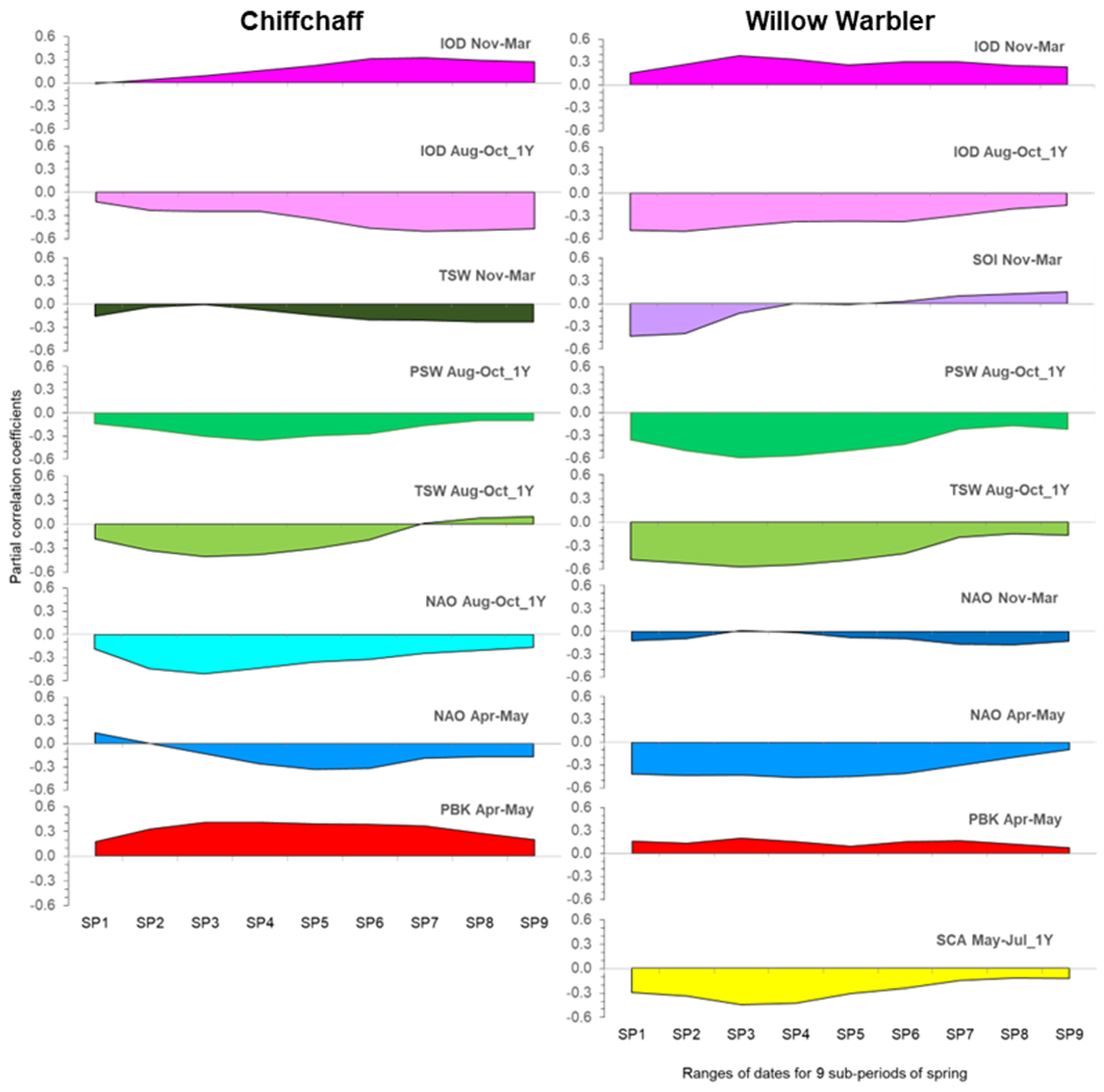
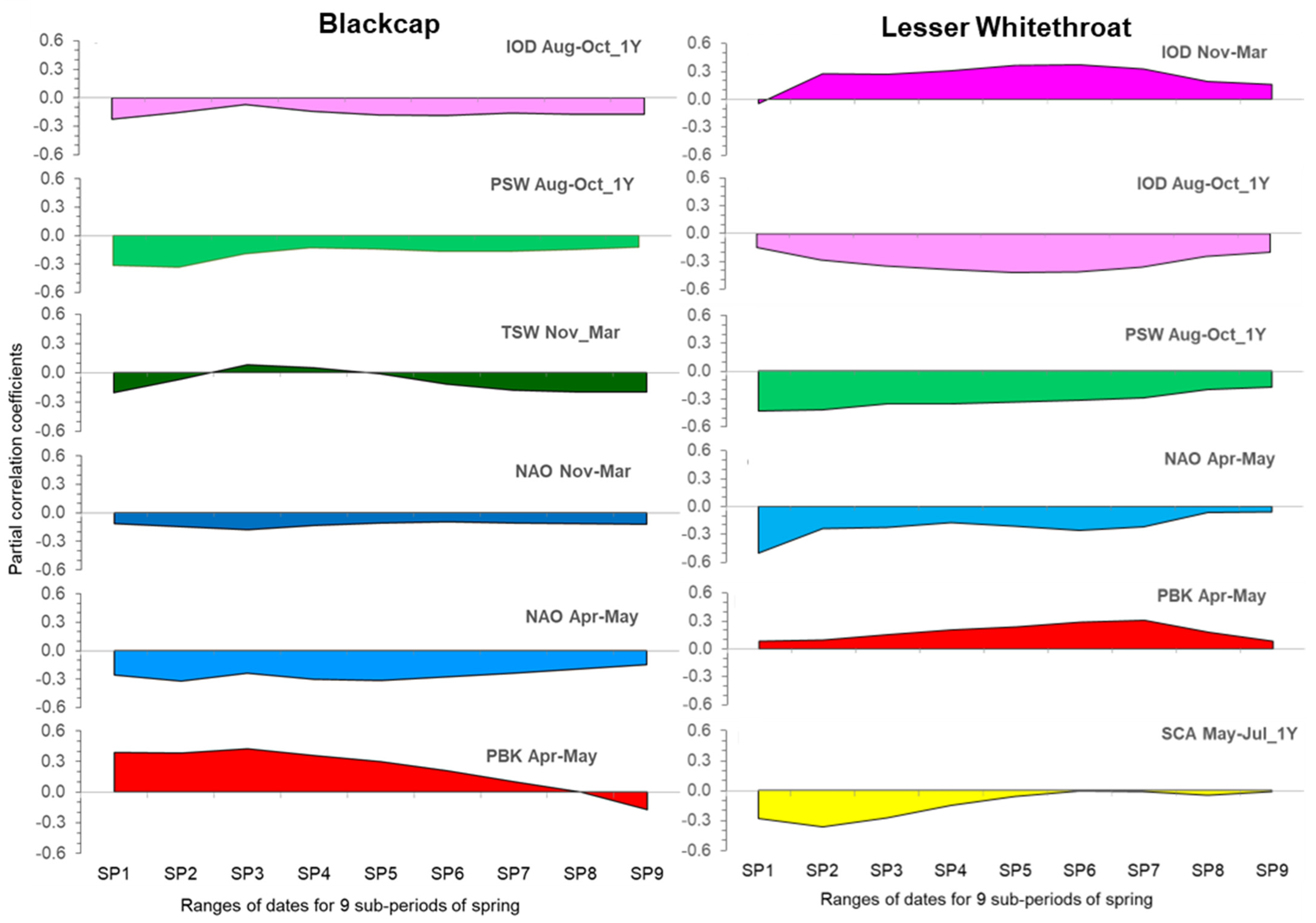
3.3. Effects of Climate Factors on Migrants in Nine Overlapping Sub-Periods of Passage (SP1–SP9)

Inspired by temporal changes in the effects of climate factors over three subsequent periods of passage, which occurred in each species (Figure 4), we set out to follow these changes in more detail and for smaller cohorts of migrants. For each species, based on the best models (Figure 4, Table 3, Table 4, Table 5 and Table 6), we selected a set of 6–9 climate variables, and we modelled their effects in the overlapping periods SP1–SP9; this contributes to a visual understanding of how the influence of each climate variable changed continuously at Bukowo through the spring migration (Figure 5 and Figure 6).

The change in the thickness of “ribbons” in different colours reflects the gradual change in the strength of the influence of each climate factor over the season (Figure 5 and Figure 6). So, for the Chiffchaff, the “narrowing” of two green ribbons reflects the decrease in the effect of precipitation and temperatures in the Western Sahel in August–October, and the “widening” of two pink ribbons reflects the increase in the influence of the IOD in August–October and in November–December; this visualizes the possible gradual change of the dominance of these effects among subsequent cohorts of arriving migrants. For the Chiffchaff, the influence of IOD in August–October manifested in the first four sub-periods (SP1–SP4, Figure 5), although with low intensity; therefore, it was not selected as one of the top models for MP1 when migrants were divided into three larger cohorts (Table 3). For the Blackcap, the influence of IOD in August–October, which occurred only for the overall passage (AA) (Figure 4, Table 5) and not when it was divided into thirds (MP1–MP3), seems to occur throughout the whole season (SP1–SP9), though with low intensity, as reflected by the narrow pink “ribbons” in Figure 6. Other than just visualizing the change of the strengths of each climate factor throughout spring, modelling influences on these factors on smaller cohorts of migrants, emphasized additional aspects of the sequence of these effects, considering that the models for sub-periods with even numbers can be directly compared, as well as those for the sub-period with the uneven numbers (Figure 5 and Figure 6).

4. Discussion

In our previous study [8], we showed that there is no one uniform set of climate indices that would universally explain the long-term changes in spring migration timing of long-distance migrants to Europe, for which wintering grounds span Africa and the Mediterranean region. In this study, we go further and suggest that even within a species, there is no one set of climate factors that explains phenological shifts over the whole spring passage of a species through a stopover site. Instead, our results indicate that the first and the last cohorts of migrants might be influenced by different climate factors, while other factors can influence the entire spring passage of a species, though with variable intensities. This intra-specific variation in arrival at the southern coast of the Baltic Sea is explained as a response to multiple climate factors influencing migrants from different regions of their wide wintering grounds and along different migration routes that cross in central Europe. We aim to explain this temporal variation in the context of current knowledge on wintering grounds and migration routes of each species. We discuss our findings in the context of climate change, which manifests differently in various parts of these species’ breeding and non-breeding ranges.

4.1. Long-Term Trends in the Overall Spring Migration Timing in the Four Species

The overall trend for earlier spring arrivals at Bukowo for the Chiffchaff, Willow Warbler, and Blackcap corresponds with analogous trend for these species reported from other locations in northwestern Europe, including Rybachy (Russia, Kaliningrad) over 1959–1990 [88], Christiansø (Denmark) over 1976–1997 [89], Helgoland (Germany, North Sea) over 1960–2002 [34], Fair Isle (Scotland) over 1955–2014 [90], and in Oxfordshire (UK) over 1971–2000 [21]. In light of our results, showing the influence of climatic conditions at remote wintering grounds on spring phenology of these species, we suggest that the advance of these species’ spring arrivals in Europe, including the Baltic region, is related not only with increasing temperatures in Europe, e.g., [91], but it is also a reflection of the long-term trends for an increase of temperatures in West Africa observed since 1950s and an increase of precipitation in the Sahel since 1980s [8]. The values of IOD in autumn and winter months have also increased over 1982–2021 [8], which reflects more frequent occurrence of its positive phase that brings easterly winds and above-average rainfall in East Africa [76,92]. In addition, some populations of Chiffchaff and Blackcap occurring at Bukowo overwinter in southern and southwestern Europe, where winters are increasingly milder [93]. These effects, in combination with increasingly earlier and warmer springs in Europe over the last several decades, might facilitate the multi-year shift to earlier arrivals, such as the trends we and other authors observed [21,34,89,90].

However, a lack of analogous multi-year trends for the Lesser Whitethroat, another insectivore long-distance migrant warbler, is striking. Lesser Whitethroats arriving in the Baltic regions overwinter more to the east than the remaining species, mostly in the Eastern Sahel, Horn of Africa, and the Middle East. These areas are under some climatic influence of the Indian Ocean Dipole [71], a climate index showing a long-term trend both for autumn and winter [8]. However, the core of this oscillation’s climatic influence is in East Africa [92], south of the main wintering range of the Lesser Whitethroat. Also, the influence of the precipitation in the Western Sahel, which has increased since the 1980s [8,69,70], on some proportion of Lesser Whitethroats arriving at Bukowo, might have incurred some long-term trend as in the other species. We attribute a lack of any multi-year phenological shifts in the spring timing of the Lesser Whitethroat at Bukowo to the influence of other climatic factors, acting closer to the breeding grounds, which show large year-to-year variation, but no long-term trends, such as the Scandinavian Pattern during the previous breeding season, and spring NAO and precipitation at Bukowo. These climatic factors operate in central Europe and the Baltic region [64], and likely fine-tune Lesser Whitethroats’ spring timing once they arrive in Europe [94], shaping the year-to-year variation we observed at Bukowo.

4.2. Sequential Effects of Climate Factors on Spring Passage on the Southern Baltic Coast in the Context of Migration Patterns of the Four Long-Distance Migrants

4.2.1. Carry-Over Effect of Conditions During the Previous Autumn and Winter on Spring Passage of the Long-Distance Migrants on the Southern Baltic Coast

In arid areas, such as the Sahara, the Sahel, and some parts of the Mediterranean region, increased precipitation has a positive influence on vegetation cover and crops, and thus on insect abundance, a few months after the rainfall [95,96,97,98]. The increased precipitation in the Sahel observed since the 1980s has already been reflected in its “greening” [69,70]. Thus, conditions for insectivorous migrants using these arid areas of Africa or the Mediterranean region, likely also improve in wet years. The delayed effect of rainfall on ecological conditions might explain the influence of conditions in the western Sahel (PSW, TSW), eastern Africa (IOD), and southeastern Africa (SOI) in August–October, when the migrants are mostly still on their way from Europe, on their passage in the Baltic region in spring, about half a year later. Increased vegetation cover should benefit Blackcaps and Lesser Whitethroats in particular as they supplement their diet with fruit while fattening for migration [13,99]. Good feeding conditions at the wintering grounds and stopover sites, in any part of Africa, likely enable migrants staying there to accumulate fuel and depart these sites early, hence arrive in Europe early in spring following such conditions. The opposite conditions, i.e., drought at wintering and stopover areas, which reduce vegetation cover and food abundance, might delay arrivals of long-distance migrants at their breeding grounds [17].

4.2.2. The Climatic Influence of Conditions in West and East Africa on the Four Species as an Evidence of the Crossroads of Western and Eastern Flyways at the Baltic Coast

For all four compared species, we revealed carry-over effects of the climatic factors that operate in West Africa (PSW, TSW) as well as those that operate in East Africa (IOD) on their spring migration phenology at the southern coast of the Baltic Sea. This supports our assumption that the Polish coast is located on the crossroads of the main migration flyways of migrants between Africa and Europe, the Western, the Central, and the Eastern Flyway [8,57,100]. Migration connectivity of all four species between populations breeding in the Baltic region and western Africa has been well documented by ringing recoveries [10]. But the underrepresented number of ringing recoveries from East Africa and along the Eastern Flyway, due to a lower chance of retrieval of a ringed bird in these areas than in western areas, has led to underestimation of the proportion of the eastern migratory populations among birds breeding in central and northern Europe [10,11,12,38,41,44]. Fortunately, growing evidence from geolocator tracking [100], orientation experiments [40], and more ringing recoveries from eastern areas of Europe and Africa [10] confirms that a considerable proportion of migrants breeding in northern and central Europe use the Eastern Flyway. Our study contributes to this growing evidence for the intraspecific mixture of migratory populations among birds breeding in this region of Europe.

4.2.3. The Variety of Climate Factors That Influence Each Species in the Context of Its Geographical Range

We suggest that the number of climate factors which shaped the phenology of spring passage of each species reflects the width of the species’ range, as Bukowo seems to support a mixture of migratory populations from any part of the species’ range which are heading for the northern breeding grounds [10,41]. Among the species we analysed, the largest number of climate indices affected the timing of spring passage of the Willow Warbler at Bukowo. This diversity of climate factors probably reflects its largest non-breeding range and the longest migration distance of some populations among the four species (Figure 1). The effect of winter SOI on the Willow Warbler’s spring phenology corresponds with the fact that this was the only species for which the wintering range extends to southern Africa (Figure 1). SOI was not selected as an influential climate variable for the other three species that do not reach that far south (Figure 1 and Figure 4). Apart from this southern extension, the Willow Warbler shares wintering grounds in other parts of Africa and Europe with the other species; it uses similar migration routes and stopover areas on the way from these areas to the Baltic region. Hence, almost all the climatic factors that influenced the passage of the other species also had effect on the Willow Warbler’s phenology.

In contrast, for Lesser Whitethroat, the influence of only three climate factors that operate at their non-breeding grounds (IOD in two seasons, and PSW) likely reflects its smallest non-breeding range among the four species (Figure 1). The other three climate factors that showed any influence on the Lesser Whitethroat were the Scandinavian Pattern, which reflects conditions in the northern part of its breeding range, and spring conditions in Europe, which likely fine-tune the final arrival dates of this species at Bukowo, as in other passerines [94,101].

4.2.4. The Temporal Changes in the Influence of Climate Factors as a Reflection of the Sequence of Passage of Different Migratory Populations

Comparison of the Climatic Effects in the Two Leaf Warblers

The difference between closely related Willow Warbler and Chiffchaff in the patterns of IOD’s influence on their arrival at Bukowo is striking. In the first species, IOD had the strongest effect on the first two-thirds of migrants (MP1–MP2), suggesting that populations arriving from the southeast of Africa and the Middle East predominantly arrive in the first cohorts of migrants. In contrast, Chiffchaffs coming from that direction seem to be in a minority at the start of passage, and their proportion increases towards the end of migration (MP2–MP3, SP5–SP9). This difference might be an effect of the much longer distances, up to 10 000 km, along the Eastern Flyway that the early-arriving populations of Willow Warblers coming from southeastern Africa have to cover, as suggested by the influence of winter SOI on their arrivals at Bukowo. These Willow Warblers would arrive at Bukowo early if they had departed from southern Africa early in anticipation of the long distance to cover and encountered good conditions on stopovers. Chiffchaffs using this flyway cover ca 4000–5000 km if they arrive from East Africa [8,10].

Regarding Chiffchaff, the influence of temperature and precipitation in the western Sahel in August–October and November–March of the previous year was the strongest for the first two-thirds of the passage (MP1–MP2, SP1–SP6); it was weaker but still evident during the final third. This most likely indicates the arrival of the nominate collybita subspecies at Bukowo from wintering grounds in West Africa [14,43,45]. The influence of NAO August–October was also strong for the first two-thirds of the passage of Chiffchaffs. This might indicate either the passage of populations of that subspecies which winter in the western part of the Mediterranean region, the Iberian Peninsula, or western Europe [14,43,45]; it might also reflect passage of the populations that are arriving from western Africa, using these areas for spring stopovers, or both. Together, these results suggest that Chiffchaffs of the nominative subspecies predominate among the first arrivals and the first two-thirds of Chiffchaffs passing through Bukowo. The effect of the IOD was small at the start of spring but increased from the second third of passage (MP2–MP3, SP5–SP9). This suggests that the abietinus subspecies, from wintering grounds in the northeastern and central Africa, the Middle East, and in the eastern Mediterranean region, tend to arrive later than the nominate subspecies [14,43,45].

It is striking that this sequence of arrival of the two subspecies of Chiffchaffs at Bukowo is the opposite to that observed at the Ottenby Bird Observatory, located in Sweden, ca 230 km north of Bukowo across the Baltic Sea [56]. Based on the pattern of climatic influences, we suggest that at Bukowo the first arriving Chiffchaffs belong mostly to the collybita subspecies, followed later by the abietinus, whereas at Ottenby, the individuals of the abietinus subspecies arrive first, from the beginning of April, but collybita birds occur only from the beginning of May onwards. One explanation for this discrepancy might be that the collybita Chiffchaffs that arrive at Bukowo already from the end of March might head for breeding grounds farther east along the southern Baltic coast or inland of it, and therefore, have no need to cross the Baltic towards the north (Figure 1D). The later occurrence, on average, of this subspecies in Ottenby than at Bukowo, might reflect the arrival at Ottenby of collybita populations breeding locally and in southern Sweden [43]. But the influence of IOD throughout the whole Chiffchaff passage at Bukowo, from 26 March onwards, corresponds well with the abietinus subspecies’ occurrence at Ottenby from about 1 April [56]. A second explanation for the difference between the results from the two Baltic stations might relate to the different time spans they cover: the Ottenby data came from 1978–1984 [56], while we analysed data from Bukowo from 1982–2024. In the light of changing wintering patterns of Chiffchaffs, for example the overwintering of collybita Chiffchaffs in the Iberian Peninsula [102] and the range expansion of this subspecies into southern Sweden observed since the 1970s [43], the arrival patterns of Chiffchaffs across the Baltic region may have changed since the study of [56].

In contrast to Chiffchaff, for the Willow Warbler, the influences of IOD and SOI in August–October were the strongest for the first two-thirds of passage, but decreased in the final third. The influences of SOI and IOD probably indicate the arrival at Bukowo of Willow Warblers from the acredula subspecies, which winters in southern and eastern Africa [50,103]. The influence of SOI, the largest during the first third of passage, suggests that these longest-distance migrants might be among the first cohorts of migrating Willow Warblers to arrive. The effect of IOD in August–October and November–March, well-pronounced over the whole passage at Bukowo, can reflect the use of sites in East Africa, where IOD operates, as stopovers by the migrants from southeastern Africa, as well as arrival of migrants that had overwintered in East Africa, likely spread over a longer period of spring. The influence of temperatures and precipitation in the Western Sahel were striking for the first two-thirds of passage and remained till the end of spring; this probably reflects the arrival of the trochilus subspecies from western Africa [50,54]. Winter NAO influenced the timing of migration only during the last third (MP3) of passage at Bukowo, which might indicate arrivals of trochilus populations using areas under climatic influence of NAO, i.e., northern Africa and southwestern Europe, as stopover sites during spring migration along the Western Flyway [50,54]. High winter NAO reflects mild and wet winters in these areas [65,66], which are likely to provide good feeding conditions a few months later, when these birds stopover there while on migration from western Africa; these conditions promote increased survival of weak and young birds, which then form the “tail” of spring passage. Local precipitation in spring (PBK April–May) had a relatively small influence on the timing of Willow Warblers’ passage in relation to the other climate factors, which corresponds with the weak effect of local spring temperatures shown in our earlier study using data on Willow Warblers from 1982–2017, where we did not use precipitation [8]. Results of both studies show that the conditions at the remote wintering sites have much greater influence on Willow Warbler spring phenology in the Baltic region than the local conditions, which likely only adjust their timing to the current local conditions [94].

The overall pattern of the sequence of influences of different climate factors on the passage of Willow Warblers through Bukowo corresponds well with the results we obtained using a shorter time series (1982–2017) [9]. However, for 1982–2024 the influence of the IOD is more spread over the whole spring in the current dataset (Figure 4 and Figure 6) than for 1982–2017, where the influence of the IOD and SOI was almost confined to the first two thirds of passage (MP1–MP2, SP1-SP6) [76,92]. This suggests that during the added springs of 2018–2024, Willow Warblers arriving from East Africa occurred not only early, but also late during spring. In five of these additional years, IOD was positive, and thus conditions in East Africa were wet and mild [76,92]. Such conditions might have promoted survival of more young or weak birds using this area to winter or stopover, which usually migrate slower than adults and fit birds [104], hence the longer spread of arrivals of Willow Warblers from areas influenced by IOD, in the current study. These results provide a hint that the influence, or relative importance, of the different climate factors might change through time. This would be an anticipated impact of global climate change on these patterns. As the length of the available time series increases, this is a topic for further study.

Comparison of the Climatic Effects in the Two Larger Warblers

The differences we found in the influence of climate factors on spring phenology of the two closely related larger warblers, the Blackcap and the Lesser Whitethroat, which use similar habitats and food [14], likely result from their different non-breeding ranges (Figure 1), but might also reflect their differences in migration strategies and plasticity in adjusting migratory behaviour to climate change [47].

Blackcap is the most flexible of the four migrants we analysed, in terms of its ability to adjust to climate change, which has manifested over recent decades in a decrease of average migration distances [105], and the establishment of new wintering grounds in the UK close to its breeding grounds in continental Europe [46]. Changes in their patterns of fuelling on migration correspond with these changes in their migration strategies and with climate-induced changes in food availability [47]. Our results correspond well with this high intraspecific plasticity, which likely differs between its long-distance and short-distance migrant populations. At Bukowo, both long-winged trans-Saharan migrants and short-winged short-distance migrant Blackcaps occur during spring and autumn passage, as demonstrated by Ożarowska and co-authors [38,40,47,106], and confirmed by ringing recoveries [10,41]. Our results, showing the response of the timing of Blackcap passage at Bukowo to different climate factors in remote wintering grounds in West or East Africa, and to winter conditions in Europe or North Africa, correspond well with these earlier findings.

The influence of precipitation and temperatures in the western Sahel, pronounced throughout the whole spring passage of Blackcaps at Bukowo, suggests that populations from the well-documented Blackcap wintering grounds in West Africa [10] pass through the southern Baltic coast during the whole spring, but likely are the most numerous among the first and the last thirds of spring migrants. The effect of IOD, which is prominent for the overall passage of Blackcap (AA) and present throughout the whole spring (SP1–SP9), corresponds with the likely arrival of Blackcaps from East Africa (which is poorly documented by ringing recoveries) and the arrival of populations wintering or using stopovers in the Middle East (which is well supported by ringing recoveries [10,41] and orientation experiments [40]. We suggest that the effects of conditions in West Africa, East Africa, and the Middle East, persistent over the whole spring, indicate the passage of the long-distance trans-Saharan migrant populations through Bukowo, which might head for breeding areas farther northeast or breed nearby [10,47].

The influence of the winter NAO (Nov–Oct), which occurs during the whole spring (SP1–SP9) but is most prominent for the last third (MP3) of Blackcaps on passage, suggests that they might belong to the short-distance migratory populations. These populations likely arrive at Bukowo from wintering grounds where the climate is shaped by NAO, i.e., from the UK or the western Mediterranean region. Geolocator tracks of Blackcaps breeding near Bukowo station also showed that these birds overwintered in the Iberian or the Apennine Peninsulas without crossing the Mediterranean Sea [39], and winter weather at both peninsulas is influenced by NAO. Thus, our results are in line with those from tracking Blackcaps. However, temperatures in West Africa also had some influence on the timing of the last third of migrants (MP3). We suggest that these last cohorts of migrants might contain a mixture of both late-arriving short-distance migrants, probably breeding locally or near Bukowo, and the late fraction of the migrants from West Africa, probably young or weak individuals, which are usually delayed on migration in comparison with adults and fit birds [104].

The influence of the spring NAO, most prominent for the middle part (MP2) but occurring throughout Blackcaps’ passage at Bukowo (for SP1–SP9), likely reflects the influence of spring conditions in central Europe, largely shaped by NAO [65], where the routes of Blackcaps arriving from any direction and heading to the northern breeding grounds meet [10].

The negative effect of local precipitation at Bukowo on passing Blackcaps, well pronounced for most of the passage (MP1–MP2 or SP1–SP6), indicates that such conditions, which in April at Bukowo might result in snow, hail, and/or large storms (MR, pers. obs.), delay most migrants [107]. The fading away of this negative influence at the end of the spring passage (MP3, SP7–SP9) suggests that these last cohorts include Blackcaps arriving from nearby stopovers despite rain. Additionally, the effect of high precipitation on migrants might be less harmful in May, which is usually warmer than April in the Baltic region [64].

We found an influence of the precipitation in the western Sahel in August-October on the Lesser Whitethroat; this was unexpected because most of the species’ non-breeding range includes East Africa and the Middle East (Figure 1B). This might be spurious, or it might indicate that wintering distribution of Lesser Whitethroats extends west of the central Sahel, with patches of its non-breeding distribution extending into this poorly-studied part of West Africa (Figure 1A,B). Additionally, several ringing recoveries of the Lesser Whitethroat between central and northern Europe and Congo [10] suggest that this species crosses the central Sahel, and hence, an influence of precipitation in the western-central Sahel on this species’ passage is not entirely impossible. Our results, showing the influence of conditions in the western Sahel, suggest that Lesser Whitethroat from the western part of its non-breeding range migrate through the Baltic region, indicating that their proportion among migrants and breeders there and farther north and northeast have been underestimated due to low rate of ringing recoveries from the central Sahel [10].

5. Conclusions

We suggest that the relationships between spring migration timing and climate indices changed sequentially during spring, and thus, we consider it likely that the Baltic coast lies on a crossroads of migration routes and supports a mixture of populations arriving sequentially from different wintering regions in Africa. Furthermore, we suggest that the drivers of the observed phenological shifts in passage through Europe are related to changes in climate during the previous breeding season, in the remote wintering grounds, along migration routes, and at stopover sites. We propose that analyses of the sequence of migrants’ passage at a stopover site will help unravel both the origins of migrants and the effects of climate factors on their arrivals at the site.

References

1. Miller-Rushing, A.J.; Lloyd-Evans, T.L.; Primack, R.B.; Satzinger, P. Bird Migration Times, Climate Change, and Changing Population Sizes. Glob. Change Biol. 2008, 14, 1959–1972. [Google Scholar] [CrossRef]
2. Usui, T.; Butchart, S.H.M.; Phillimore, A.B. Temporal Shifts and Temperature Sensitivity of Avian Spring Migratory Phenology: A Phylogenetic Meta-Analysis. J. Anim. Ecol. 2017, 86, 250–261. [Google Scholar] [CrossRef]
3. Gordo, O.; Sanz, J.J. Climate Change and Bird Phenology: A Long-Term Study in the Iberian Peninsula. Glob. Change Biol. 2006, 12, 1993–2004. [Google Scholar] [CrossRef]
4. Saino, N.; Ambrosini, R.; Rubolini, D.; Von Hardenberg, J.; Provenzale, A.; Hüppop, K.; Hüppop, O.; Lehikoinen, A.; Lehikoinen, E.; Rainio, K.; et al. Climate warming, ecological mismatch at arrival and population decline in migratory birds. Proc. R. Soc. B Biol. Sci. R. Soc. 2011, 278, 835–842. [Google Scholar] [CrossRef] [PubMed]
5. Gordo, O.; Brotons, L.; Ferrer, X.; Comas, P. Do Changes in Climate Patterns in Wintering Areas Affect the Timing of the Spring Arrival of Trans-Saharan Migrant Birds? Glob. Change Biol. 2005, 11, 12–21. [Google Scholar] [CrossRef]
6. Saino, N.; Ambrosini, R. Climatic Connectivity between Africa and Europe May Serve as a Basis for Phenotypic Adjustment of Migration Schedules of Trans-Saharan Migratory Birds. Glob. Change Biol. 2008, 14, 250–263. [Google Scholar] [CrossRef]
7. Remisiewicz, M.; Underhill, L.G. Climatic Variation in Africa and Europe Has Combined Effects on Timing of Spring Migration in a Long-Distance Migrant Willow Warbler Phylloscopus trochilus. PeerJ 2020, 8, e8770. [Google Scholar] [CrossRef] [PubMed]
8. Remisiewicz, M.; Underhill, L.G. Large-Scale Climatic Patterns Have Stronger Carry-Over Effects than Local Temperatures on Spring Phenology of Long-Distance Passerine Migrants between Europe and Africa. Animals 2022, 12, 1732. [Google Scholar] [CrossRef]
9. Remisiewicz, M.; Underhill, L.G. Climate in Africa Sequentially Shapes Spring Passage of Willow Warbler Phylloscopus trochilus across the Baltic Coast. PeerJ 2022, 10, e12964. [Google Scholar] [CrossRef]
10. Spina, F.; Baillie, S.R.; Bairlein, F.; Fiedler, W.; Thorup, K. (Eds.) The Eurasian African Bird Migration Atlas. 2022. Available online: https://migrationatlas.org/ (accessed on 23 July 2025).
11. Valkama, J.; Saurola, P.; Lehikoinen, A.; Lehikoinen, E.; Piha, M.; Sola, P.; Velmala, W. Suomen Rengastysatlas. [The Finnish Bird Ringing Atlas]; Finnish Museum of Natural History and Ministry of Environment: Helsinki, Finland, 2014; Volume II. [Google Scholar]
12. Fransson, T.; Hall-Karlsson, S. Svensk Ringmärkningsatlas; Naturhistoriska riksmuseet & Sveriges Ornitologiska Forening: Stockholm, Sweden, 2008; Volume 3. [Google Scholar]
13. Zwarts, L.; Bijlsma, R.G.; van der Kamp, J.; Wymenga, E. Living on the Edge: Wetlands and Birds in a Changing Sahel; KNNV Publishing: Zeist, The Netherlands, 2009. [Google Scholar]
14. Cramp, S.; Brooks, D.J. The Birds of the Western Palearctic. In Handbook of the Birds of Europe, the Middle East and North Africa; Oxford University Press: Oxford, UK, 1992; Volume VI: Warblers. [Google Scholar]
15. Hušek, J.; Adamík, P.; Cepák, J.; Tryjanowski, P. The Influence of Climate and Population Size on the Distribution of Breeding Dates in the Red-Backed Shrike (Lanius collurio). Ann. Zool. Fennici 2009, 46, 439–450. [Google Scholar] [CrossRef]
16. Tryjanowski, P.; Stenseth, N.C.; Matysioková, B. The Indian Ocean Dipole as an Indicator of Climatic Conditions Affecting European Birds. Clim. Res. 2013, 57, 45–49. [Google Scholar] [CrossRef]
17. Tøttrup, A.P.; Klaassen, R.H.G.; Kristensen, M.W.; Strandberg, R.; Vardanis, Y.; Lindström, Å.; Rahbek, C.; Alerstam, T.; Thorup, K. Drought in Africa Caused Delayed Arrival of European Songbirds. Science 2012, 338, 1307. [Google Scholar] [CrossRef] [PubMed]
18. Tobolka, M.; Dylewski, L.; Wozna, J.T.; Zolnierowicz, K.M. How Weather Conditions in Non-Breeding and Breeding Grounds Affect the Phenology and Breeding Abilities of White Storks. Sci. Total Environ. 2018, 636, 512–518. [Google Scholar] [CrossRef]
19. Askeyev, O.V.; Sparks, T.H.; Askeyev, I.V.; Tryjanowski, P. Spring Migration Timing of Sylvia Warblers in Tatarstan (Russia) 1957–2008. Cent. Eur. J. Biol. 2009, 4, 595–602. [Google Scholar] [CrossRef]
20. Askeyev, O.V.; Sparks, T.H.; Askeyev, I.V.; Tryjanowski, P. Is Earlier Spring Migration of Tatarstan Warblers Expected under Climate Warming? Int. J. Biometeorol. 2007, 51, 459–463. [Google Scholar] [CrossRef]
21. Cotton, P.A. Avian Migration Phenology and Global Climate Change. Proc. Natl. Acad. Sci. USA 2003, 100, 12219–12222. [Google Scholar] [CrossRef]
22. Saino, N.; Rubolini, D.; Jonzén, N.; Ergon, T.; Montemaggiori, A.; Stenseth, N.C.; Spina, F. Temperature and Rainfall Anomalies in Africa Predict Timing of Spring Migration in Trans-Saharan Migratory Birds. Clim. Res. 2007, 35, 123–134. [Google Scholar] [CrossRef]
23. Haest, B.; Hüppop, O.; Bairlein, F. Weather at the Winter and Stopover Areas Determines Spring Migration Onset, Progress, and Advancements in Afro-Palearctic Migrant Birds. Proc. Natl. Acad. Sci. USA 2020, 117, 17056–17062. [Google Scholar] [CrossRef] [PubMed]
24. Tomotani, B.M.; van der Jeugd, H.; Gienapp, P.; de la Hera, I.; Pilzecker, J.; Teichmann, C.; Visser, M.E. Climate Change Leads to Differential Shifts in the Timing of Annual Cycle Stages in a Migratory Bird. Glob. Change Biol. 2018, 24, 823–835. [Google Scholar] [CrossRef] [PubMed]
25. Redlisiak, M.; Remisiewicz, M.; Nowakowski, J.K. Long-Term Changes in Migration Timing of Song Thrush Turdus Philomelos at the Southern Baltic Coast in Response to Temperatures on Route and at Breeding Grounds. Int. J. Biometeorol. 2018, 62, 1595–1605. [Google Scholar] [CrossRef]
26. Ouwehand, J.; Both, C. African Departure Rather than Migration Speed Determines Variation in Spring Arrival in Pied Flycatchers. J. Anim. Ecol. 2017, 86, 88–97. [Google Scholar] [CrossRef]
27. Remisiewicz, M.; Bernitz, Z.; Bernitz, H.; Burman, M.S.; Raijmakers, J.M.H.; Raijmakers, J.H.F.A.; Underhill, L.G.; Rostkowska, A.; Barshep, Y.; Soloviev, S.A.; et al. Contrasting Strategies for Wing-Moult and Pre-Migratory Fuelling in Western and Eastern Populations of Common Whitethroat Sylvia Communis. Ibis 2019, 161, 824–838. [Google Scholar] [CrossRef]
28. Alerstam, T. Bird Migration; Cambridge University Press: Cambridge, UK, 1993. [Google Scholar]
29. Gill, F.B. Ornithology, 3rd ed.; W. H. Freeman and Company: New York, NY, USA, 2006. [Google Scholar]
30. O’Connor, R.S.; Love, O.P.; Régimbald, L.; Le Pogam, A.; Gerson, A.R.; Elliott, K.H.; Hargreaves, A.L.; Vézina, F. An Arctic Breeding Songbird Overheats during Intense Activity Even at Low Air Temperatures. Sci. Rep. 2024, 14, 15193. [Google Scholar] [CrossRef] [PubMed]
31. Zwarts, L.; Bijlsma, R.G.; Van Der Kamp, J. The Fortunes of Migratory Birds from Eurasia: Being on a Tightrope in the Sahel. Ardea 2023, 111, 397–437. [Google Scholar] [CrossRef]
32. Allan, D.G.; Harrison, J.A.; Herremans, M.; Navarro, R.; Underhill, L.G. Southern African Geography: Its Relevance to Birds. In The Atlas of Southern African Birds Volume 1: Non-Passerines; Harrison, J.A., Allan, D.G., Underhill, L.G., Herremans, M., Tree, A.J., Parker, V., Brown, C.J., Eds.; BirdLife South Africa: Johannesburg, South Africa, 1997. [Google Scholar]
33. Katti, M.; Price, T. Annual Variation in Fat Storage by a Migrant Warbler Overwintering in the Indian Tropics. J. Anim. Ecol. 1999, 68, 815–823. [Google Scholar] [CrossRef]
34. Hüppop, O.; Hüppop, K. North Atlantic Oscillation and Timing of Spring Migration in Birds. Proc. R. Soc. B Biol. Sci. 2003, 270, 233–240. [Google Scholar] [CrossRef] [PubMed]
35. Stenseth, N.C.; Ottersen, G.; Hurrell, J.W.; Mysterud, A.; Lima, M.; Chan, K.S.; Yoccoz, N.G.; Ådlandsvik, B. Studying Climate Effects on Ecology through the Use of Climate Indices: The North Atlantic Oscillation, El Niño Southern Oscillation and Beyond. Proc. R. Soc. B Biol. Sci. 2003, 270, 2087–2096. [Google Scholar] [CrossRef]
36. Haest, B.; Hüppop, O.; Bairlein, F. Challenging a 15-Year-Old Claim: The North Atlantic Oscillation Index as a Predictor of Spring Migration Phenology of Birds. Glob. Change Biol. 2018, 24, 1523–1537. [Google Scholar] [CrossRef]
37. Trepte, A. Avi-Fauna—Vögel in Deutschland. Available online: https://www.avi-fauna.info/ (accessed on 23 July 2025).
38. Kopiec, K.; Ożarowska, A. The Origin of Blackcaps Sylvia atricapilla Wintering on the British Isles. Ornis Fenn. 2012, 4, 254–263. [Google Scholar] [CrossRef]
39. Delmore, K.E.; Van Doren, B.M.; Conway, G.J.; Curk, T.; Garrido-Garduño, T.; Germain, R.R.; Hasselmann, T.; Hiemer, D.; van der Jeugd, H.P.; Justen, H.; et al. Individual Variability and Versatility in an Eco-Evolutionary Model of Avian Migration. Proc. R. Soc. B Biol. Sci. 2020, 287, 20201339. [Google Scholar] [CrossRef]
40. Ożarowska, A.; Yosef, R.; Busse, P. Orientation of Chiffchaff (Phylloscopus collybita), Blackcap (Sylvia atricapilla) and Lesser Whitethroat (S. curruca) on Spring Migration at Eilat, Israel. Avian Ecol. Behav. 2004, 12, 1–10. [Google Scholar]
41. Maciąg, T.; Remisiewicz, M.; Nowakowski, J.K.; Redlisiak, M.; Rosińska, K.; Stępniewski, K.; Stępniewska, K.; Szulc, J. Maps of Ringing Recoveries. Website of the Bird Migration Research Station. Available online: https://en-sbwp.ug.edu.pl/badania/monitoringwyniki/maps-of-ringing-recoveries/ (accessed on 23 July 2025).
42. Lerche-Jørgensen, M.; Willemoes, M.; Tøttrup, A.P.; Snell, K.R.S.; Thorup, K. No Apparent Gain from Continuing Migration for More than 3000 Kilometres: Willow Warblers Breeding in Denmark Winter across the Entire Northern Savannah as Revealed by Geolocators. Mov. Ecol. 2017, 5, 17. [Google Scholar] [CrossRef]
43. Hansson, M.C.; Bensch, S.; Brännström, O. Range Expansion and the Possibility of an Emerging Contact Zone between Two Subspecies of Chiffchaff Phylloscopus collybita ssp. J. Avian Biol. 2000, 31, 548–558. [Google Scholar] [CrossRef]
44. Bakken, V.; Runde, O.J.; Tjørve, E.; Koblik, E.A. Norsk Ringmerkingsatlas; Stavanger Museum: Stavanger, Norway, 2003; Volume 1. [Google Scholar]
45. Ciach, M. Leaf Warblers (Phylloscopus spp.) As a Model Group in Migration Ecology Studies. Ring 2009, 31, 3–13. [Google Scholar] [CrossRef]
46. Berthold, P.; Terrill, S.B. Migratory Behaviour and Population Growth of Blackcaps Wintering in Britain and Ireland: Some Hypotheses. Ringing Migr. 1988, 9, 153–159. [Google Scholar] [CrossRef]
47. Ożarowska, A.; Meissner, W. Increasing Body Condition of Autumn Migrating Eurasian Blackcaps Sylvia Atricapilla over Four Decades. Eur. Zool. J. 2024, 91, 151–161. [Google Scholar] [CrossRef]
48. Ożarowska, A. Contrasting fattening strategies in related migratory species: The blackcap, garden warbler, common whitethroat and lesser whitethroat. Ann. Zool. Fenn. 2015, 52, 115–127. [Google Scholar] [CrossRef]
49. Hedenström, A.; Pettersson, J. Migration Routes and Wintering Areas of Willow Warblers Phylloscopus trochilus (L.) Ringed in Fennoscandia. Ornis Fenn. 1987, 64, 137–143. [Google Scholar]
50. Zhao, T.; Ilieva, M.; Larson, K.; Lundberg, M.; Neto, J.M.; Sokolovskis, K.; Åkesson, S.; Bensch, S. Autumn Migration Direction of Juvenile Willow Warblers (Phylloscopus t. trochilus and P. t. acredula) and Their Hybrids Assessed by QPCR SNP Genotyping. Mov. Ecol. 2020, 8, 22. [Google Scholar] [CrossRef]
51. Bensch, S.; Andersson, T.; Akesson, S. Morphological And Molerecular Variaton Across a Migratory Divide in Willow Warblers, Phylloscopus trochilus. Evolution 1999, 53, 1925–1935. [Google Scholar] [CrossRef] [PubMed]
52. Tomiałojć, L.; Stawarczyk, T. Awifauna Polski: Rozmieszczenie, Liczebność i Zmiany; PTPP “pro Natura”: Wrocław, Poland, 2003. [Google Scholar]
53. Bensch, S.; Bengtsson, G.; Åkesson, S. Patterns of Stable Isotope Signatures in Willow Warbler Phylloscopus trochilus Feathers Collected in Africa. J. Avian Biol. 2006, 37, 323–330. [Google Scholar] [CrossRef]
54. Bensch, S.; Grahn, M.; MÜller, N.; Gay, L.; Åkesson, S. Genetic, Morphological, and Feather Isotope Variation of Migratory Willow Warblers Show Gradual Divergence in a Ring. Mol. Ecol. 2009, 18, 3087–3096. [Google Scholar] [CrossRef]
55. Lindström, Å.; Svensson, S.; Green, M.; Ottval, R. Distribution and Population Changes of Two Subspecies of Chiffchaff Phylloscopus collybita in Sweden. Ornis Svec. 2007, 17, 137–147. [Google Scholar] [CrossRef]
56. Ellergren, H.; Pettersson, J. Gransångarens Phylloscopus colybita Vårforekomst Vid Ottenby. Calidris 1985, 14, 3–12. [Google Scholar]
57. Busse, P.; Meissner, W. Bird Ringing Station Manual; De Gruyter Open Ltd.: Warsaw, Poland; Berlin, Germany, 2015. [Google Scholar]
58. Demongin, L. Identification Guide to Birds in the Hand; Laurent Demongin: Beauregard-Vendon, France, 2016. [Google Scholar]
59. Svensson, L. Identification Guide to European Passerines; British Trust for Ornithology: Thetford, UK, 1992. [Google Scholar]
60. Pinszke, A.; Remisiewicz, M. Long-Term Changes in Autumn Migration Timing of Garden Warblers Sylvia borin at the Southern Baltic Coast in Response to Spring, Summer and Autumn Temperatures. Eur. Zool. J. 2023, 90, 283–295. [Google Scholar] [CrossRef]
61. Gołębiewski, I.; Remisiewicz, M. Carry-Over Effects of Climate Variability at Breeding and Non-Breeding Grounds on Spring Migration in the European Wren Troglodytes troglodytes at the Baltic Coast. Animals 2023, 13, 2015. [Google Scholar] [CrossRef]
62. Barstone, A.G.; Livezey, R.E. Classification, Seasonality and Persistence of Low–Frequency Atmospheric Circulation Patterns. Mon. Weather Rev. 1987, 115, 1083–1126. [Google Scholar]
63. Bueh, C.; Nakamura, H. Scandinavian Pattern and Its Climatic Impact. Q. J. R. Meteorol. Soc. 2007, 133, 2117–2131. [Google Scholar] [CrossRef]
64. Markus Meier, H.E.; Kniebusch, M.; Dieterich, C.; Gröger, M.; Zorita, E.; Elmgren, R.; Myrberg, K.; Ahola, M.P.; Bartosova, A.; Bonsdorff, E.; et al. Climate Change in the Baltic Sea Region: A Summary. Earth Syst. Dyn. 2022, 13, 457–593. [Google Scholar] [CrossRef]
65. Hurrell, J.W. Decadal Trends in the North Atlantic Oscillation: Regional Temperatures and Precipitation. Science 1995, 269, 676–679. [Google Scholar] [CrossRef]
66. Osborn, T.J. Recent Variations in the Winter North Atlantic Oscillation. Weather 2006, 61, 353–355. [Google Scholar] [CrossRef]
67. Wang, L.; Ting, M. Stratosphere-Troposphere Coupling Leading to Extended Seasonal Predictability of Summer North Atlantic Oscillation and Boreal Climate. Geophys. Res. Lett. 2022, 49. [Google Scholar] [CrossRef]
68. Simpson, I.; Hanna, E.; Baker, L.; Sun, Y.; Wei, H. North Atlantic Atmospheric Circulation Indices: Links with Summer and Winter Temperature and Precipitation in North-west Europe, Including Persistence and Variability. Int. J. Climatol. 2024, 44, 902–922. [Google Scholar] [CrossRef]
69. Wang, S.Y.; Gillies, R.R. Observed Change in Sahel Rainfall, Circulations, African Easterly Waves, and Atlantic Hurricanes since 1979. Int. J. Geophys. 2011, 2011, 1–14. [Google Scholar] [CrossRef]
70. Biasutti, M. Rainfall Trends in the African Sahel: Characteristics, Processes, and Causes. Wiley Interdiscip. Rev. Clim. Change 2019, 10, e591. [Google Scholar] [CrossRef] [PubMed]
71. Saji, N.H.; Goswami, B.N.; Vinayachandran, P.N.; Yamagata, T. A dipole mode in the tropical Indian Ocean. Nature 1999, 401, 360–363. [Google Scholar] [CrossRef] [PubMed]
72. Marchant, R.; Mumbi, C.; Behera, S.; Yamagata, T. The Indian Ocean Dipole-The Unsung Driver of Climatic Variability in East Africa. Afr. J. Ecol. 2007, 45, 4–16. [Google Scholar] [CrossRef]
73. Stige, L.C.; Stave, J.; Chan, K.-S.; Ciannelli, L.; Pettorelli, N.; Glantz, M.; Herren, H.R.; Stenseth, N.C. The Effect of Climate Variation on Agro-Pastoral Production in Africa. Proc. Natl. Acad. Sci. USA 2006, 103, 3049–3053. [Google Scholar] [CrossRef]
74. Swapna, P.; Sandeep, N.; Alsumaina, K.N.; Krishnan, R.; Ajinkya, A.; Shamal, M.; Sreejith, O.P. Contrasting tropical precipitation and ecosystem response to Indian Ocean Dipole in a warming climate. Sci. Total Environ. 2025, 971, 179081. [Google Scholar] [CrossRef]
75. McPhaden, M.J.; Santoso, A.; Cai, W. El Niño Southern Oscillation in a Changing Climate; John Wiley and Sons, Inc.: Hoboken, NJ, USA, 2021; ISBN 9781119548126. [Google Scholar]
76. NOAA National Oceanic and Atmospheric Administration US Department of Commerce National Weather Service. Climate Prediction Center. Climate & Weather Linkage. Available online: https://www.cpc.ncep.noaa.gov/ (accessed on 31 May 2025).
77. Maciag, T.; Remisiewicz, M. Climate Change Impact on the Populations of Goldcrest Regulus regulus and Firecrest Regulus ignicapilla Migrating Through the Southern Baltic Coast. Sustainability 2025, 17, 1243. [Google Scholar] [CrossRef]
78. Gould, L.A.; Manning, A.D.; McGinness, H.M.; Hansen, B.D. A Review of Electronic Devices for Tracking Small and Medium Migratory Shorebirds. Anim. Biotelemetry 2024, 12, 11. [Google Scholar] [CrossRef]
79. Finch, T.; Pearce-Higgins, J.W.; Leech, D.I.; Evans, K.L. Carry-over Effects from Passage Regions Are More Important than Breeding Climate in Determining the Breeding Phenology and Performance of Three Avian Migrants of Conservation Concern. Biodivers. Conserv. 2014, 23, 2427–2444. [Google Scholar] [CrossRef]
80. Dormann, C.F.; Elith, J.; Bacher, S.; Buchmann, C.; Carl, G.; Carré, G.; Marquéz, J.R.G.; Gruber, B.; Lafourcade, B.; Leitão, P.J.; et al. Collinearity: A Review of Methods to Deal with It and a Simulation Study Evaluating Their Performance. Ecography 2013, 36, 27–46. [Google Scholar] [CrossRef]
81. Bartoń, K. MuMIn: Multi-Model Inference. R Package Version 1.48.11: 2025. Available online: https://CRAN.R-project.org/package=MuMIn (accessed on 24 July 2025).
82. Frost, J. Regression Analysis. An Intuitive Guide for Using and Interpreting Linear Models, 1st ed. 2019. Available online: https://www.amazon.com/dp/1735431184?asin=1735431184&revisionId=&format=4&depth=1 (accessed on 24 July 2025).
83. Crawley, M.J. The R Book; John Wiley & Sons: Chichester, UK, 2013. [Google Scholar]
84. Pareto, A. R Script. Available online: https://rpubs.com/ratherbit/102428 (accessed on 30 June 2025).
85. Tukey, J. We Need Both Exploratory and Confirmatory. Am. Stat. 1980, 34, 352–354. [Google Scholar] [CrossRef]
86. Sparks, T.H.; Tryjanowski, P. The Detection of Climate Impacts: Some Methodological Considerations. Int. J. Climatol. 2005, 25, 271–277. [Google Scholar] [CrossRef]
87. R Core Team. R: A Language and Environment for Statistical Computing; R Core Team: Vienna, Austria, 2025. [Google Scholar]
88. Sokolov, L.V.; Markovets, M.Y.; Shapoval, A.P.; Morozov, Y.G. Long-Term Trends in the Timing of Spring Migration of Passerines on the Courish Spit of the Baltic Sea. Avian Ecol. Behav. 1998, 1, 1–21. [Google Scholar]
89. Tøttrup, A.P.; Thorup, K.; Rahbek, C. Patterns of change in timing of spring migration in North European songbird populations. J. Avian Biol. 2006, 37, 84–92. [Google Scholar] [CrossRef]
90. Miles, W.T.S.; Bolton, M.; Davis, P.; Dennis, R.; Broad, R.; Robertson, I.; Riddiford, N.J.; Harvey, P.V.; Riddington, R.; Shaw, D.N.; et al. Quantifying Full Phenological Event Distributions Reveals Simultaneous Advances, Temporal Stability and Delays in Spring and Autumn Migration Timing in Long-Distance Migratory Birds. Glob. Change Biol. 2017, 23, 1400–1414. [Google Scholar] [CrossRef]
91. Ockendon, N.; Leech, D.; Pearce-Higgins, J.W. Climatic Effects on Breeding Grounds Are More Important Drivers of Breeding Phenology in Migrant Birds than Carryover Effects from Wintering Grounds. Biol. Lett. 2013, 9, 0669. [Google Scholar] [CrossRef] [PubMed]
92. Hirons, L.; Turner, A. The Impact of Indian Ocean Mean-State Biases in Climate Models on the Representation of the East African Short Rains. J. Clim. 2018, 31, 6611–6631. [Google Scholar] [CrossRef]
93. ECMWF. European Centre for Medium-Range Weather Forecasts. Copernicus Services Copernicus: Global Sea Ice Cover at a Record Low and Third-Warmest February Globally. Available online: https://climate.copernicus.eu/copernicus-global-sea-ice-cover-record-low-and-third-warmest-february-globally (accessed on 9 June 2025).
94. Tøttrup, A.P.; Rainio, K.; Coppack, T.; Lehikoinen, E.; Rahbek, C.; Thorup, K. Local Temperature Fine-Tunes the Timing of Spring Migration in Birds. Proc. Integr. Comp. Biol. 2010, 50, 293–304. [Google Scholar] [CrossRef]
95. Peach, W.; Baillie, S.; Underhill, L.G. Survival of British Sedge Warblers Acrocephalus schoenobaenus in Relation to West African Rainfall. Ibis 1991, 133, 300–305. [Google Scholar] [CrossRef]
96. Maselli, F. Monitoring Forest Conditions in a Protected Mediterranean Coastal Area by the Analysis of Multiyear NDVI Data. Remote Sens. Environ. 2004, 89, 423–433. [Google Scholar] [CrossRef]
97. Bartsch, S.; Stegehuis, A.I.; Boissard, C.; Lathière, J.; Peterschmitt, J.-Y.; Reiter, I.M.; Gauquelin, T.; Baldy, V.; Genesio, L.; Matteucci, G.; et al. Impact of Precipitation, Air Temperature and Abiotic Emissions on Gross Primary Production in Mediterranean Ecosystems in Europe. Eur. J. For. Res. 2020, 139, 111–126. [Google Scholar] [CrossRef]
98. Peñuelas, J. Phenology Feedbacks on Climate Change. Science 2009, 324, 887–888. [Google Scholar] [CrossRef]
99. Berthold, P. Control of Bird Migration; Springer Science & Business Media: Berlin/Heidelberg, Germany, 1996. [Google Scholar]
100. Briedis, M.; Bauer, S.; Adamík, P.; Alves, J.A.; Costa, J.S.; Emmenegger, T.; Gustafsson, L.; Koleček, J.; Krist, M.; Liechti, F.; et al. Broad-Scale Patterns of the Afro-Palaearctic Landbird Migration. Glob. Ecol. Biogeogr. 2020, 29, 722–735. [Google Scholar] [CrossRef]
101. Briedis, M.; Hahn, S.; Adamík, P. Cold Spell En Route Delays Spring Arrival and Decreases Apparent Survival in a Long-Distance Migratory Songbird. BMC Ecol. 2017, 17, 11. [Google Scholar] [CrossRef] [PubMed]
102. Catry, P.; Bearhop, S.; Lecoq, M. Sex Differences in Settlement Behaviour and Condition of Chiffchaffs Phylloscopus Collybita at a Wintering Site in Portugal. Are Females Doing Better? J. Ornithol. 2007, 148, 241–249. [Google Scholar] [CrossRef]
103. Herremans, M. Willow Warbler Phylloscopus trochilus. In The Atlas of Southern African Birds; Harrison, J.A., Allan, D.G., Underhill, L.G., Herremans, M., Tree, A.J., Parker, V., Brown, C.J., Eds.; BirdLife: Johannesburg, South Africa, 1999; Volume 2: Passerines, pp. 254–267. [Google Scholar]
104. Alerstam, T. Bird Migration Speed. In Avian Migration; Springer: Berlin/Heidelberg, Germany, 2003; pp. 253–267. [Google Scholar]
105. Pulido, F.; Berthold, P. Microevolutionary Response to Climatic Change. Adv. Ecol. Res. 2004, 35, 151–183. [Google Scholar] [CrossRef]
106. Ożarowska, A.; Zaniewicz, G.; Meissner, W. Sex and Age Specific Differences in Wing Pointedness and Wing Length in Blackcaps Sylvia atricapilla Migrating through the Southern Baltic Coast. Curr. Zool. 2020, 67, 271–277. [Google Scholar] [CrossRef] [PubMed]
107. Elkins, N. Weather and Bird Behaviour, 2nd ed.; Poyser: London, UK, 2018. [Google Scholar]
108. Nowakowski, J. Ringing Data from the Bird Migration Research Station, University of Gdańsk. University of Gdańsk. 2017. (GBIF.org). Occurrence Dataset. Available online: https://doi.org/10.15468/q5o88l (accessed on 9 June 2025).
109. Benjamini, Y.; Hochberg, Y. Controlling the false discovery rate: A practical and powerful approach to multiple testing. J. R. Stat. Soc. Ser. B 1995, 57, 289–300. [Google Scholar] [CrossRef]
Figure 2. Visual representation of the method of dividing the overall Annual Anomaly (AA) of the entire spring passage (entire grey area) into partial anomalies for the three main periods (MP1–MP3) and nine sub-periods (SP1–SP9), using the example of the cumulative curve of spring passage in 1996 (blue line) in relation to the many-year (1982–2024) average curve of spring passage (red line), for the Willow Warbler Phylloscopus trochilus at Bukowo. Grey areas within the thick-line rectangles reflect the anomalies for the main periods (MP1–MP3), which sum up to the overall grey area, reflected by the value of AA. Grey areas within the sub-periods with uneven numbers (SP1, SP3, SP5, SP7, SP9; thin line rectangles) also sum up to the whole grey area for AA; grey areas within the sub-periods with even numbers (SP2, SP4, SP6, SP8; dashed line rectangles) also sum up to the total grey area for AA.
Diversity 17 00528 g002
Figure 3. Year-to-year variation (black circles) and long-term trends (blue lines) for the overall Annual Anomaly (AA) of spring migration for four long-distance migrant species at Bukowo (N Poland) over 1982–2024. (A) Chiffchaff Phylloscopus collybita; (B) Willow Warbler P. trochilus; (C) Blackcap Sylvia atricapilla; (D) Lesser Whitethroat Curruca curruca. * = Statistically significant regression equations (p < 0.05). The details of the regression statistics are presented in Table A3.
Diversity 17 00528 g003
Figure 4. Partial correlation coefficients (pR) for the effect of the climate variables selected in the best multiple regression models for the overall Annual Anomaly (AA) and for anomalies for the three main periods (MP1–MP3) of spring migration for the four long-distance migrant species at Bukowo (N Poland) over 1982–2024. The details of these models are presented in Table 2, Table 3 and Table 4. (A) Results of the best models for the Chiffchaff Phylloscopus collybita; (B) Results of the best models for the Willow Warbler P. trochilus; (C) Results of the best models for the Blackcap Sylvia atricapilla; (D) Results of the best models for the Lesser Whitethroat Curruca curruca. The symbols of climate variables in the Legend are as in Table 1.
Diversity 17 00528 g004
Figure 5. Partial correlation coefficients (pR) for AA in nine overlapping sub-periods (SP1–SP9) of spring migration at Bukowo, Poland, 1982–2024 for four long-distance migrant species, against the species-specific set of climate indices, based on best models for three main periods (MP1–MP3) for Chiffchaff and Willow Warbler. Symbols of climate indices as in Table 1, dates and symbols of sub-periods of spring are in Table 2, best models for each species are in Table 3 and Table 4, and are visualized in Figure 4.
Diversity 17 00528 g005
Figure 6. Partial correlation coefficients for AA in nine overlapping sub-periods (SP1–SP9) of spring migration at Bukowo, Poland, 1982–2024 for four long-distance migrant species, against the species-specific set of climate indices, based on best models for three main periods (MP1–MP3) for the Blackcap and the Lesser Whitethroat. Symbols of climate indices as in Table 1, dates and symbols of sub-periods of spring in Table 2, best models for each species are in Table 5 and Table 6, and are visualized in Figure 4.
Diversity 17 00528 g006